Office hours: Tuesdays and Thursdays: right after class (zoom)
0.2 Course Web Page
There is a web site for the course.
You can find it from my home page, which is listed above, or from
the department's home page.
You can find these lecture notes on the course home page.
Please let me know if you can't find them.
The notes are updated as bugs are found or improvements made.
As a result, I do not recommend printing the notes now (if at
all).
I will place markers at the end of each lecture after the
lecture is given.
For example, the Start Lecture #01 marker above can be
thought of as End Lecture #00.
0.3 Textbooks
In previous semesters, the course text was Tanenbaum, "Modern Operating
Systems", Forth Edition (4e).
We will cover nearly all of the first six chapters, plus some
material from later chapters.
The only real problem with that text book is its cost.
These notes are based on Tanenbaum's book; so it is not necessary for
you to buy the book.
You may wish to purchase this book but it may not be cost
effective given my class notes.
A very modern online text, which is quite good is Three Easy
Pieces http://pages.cs.wisc.edu/~remzi/OSTEP/
It is available for free online http://www.ostep.org
You are required to get it.
The three easy pieces are virtualization (recall
virtual memory from 201), concurrency (think of
processes and threads), and persistence (files and
filesystems).
Grades are based on the labs and exams; the weighting will be
approximately
20%*LabAverage + 35%*MidtermExam + 45%*FinalExam (but see homeworks
below).
0.5 Homeworks and Labs
I make a distinction between homeworks and labs.
Labs are
Required.
Computer programs you must write in C (or C++).
Due several lectures later (date given on assignment).
Announced in the notes and during class class.
Details in NYU Brightspace with supplemental material on separate web
pages.
Your solution is submitted via NYU Brightspace.
Graded and form part of your final grade.
Penalized for lateness: 2 points per day up to 5 days; then 5 points
per day.
Required to contain a README file telling the
grader how to compile and run your lab.
Homeworks are
Optional.
Mostly from the book.
Due 5PM one week after being assigned.
Not accepted late.
The assignment is given in the notes and NYU Brightspace; your
solution is submitted via Brightspace.
Checked for completeness and graded 0/1/2.
Able to help, but not hurt, your final grade.
0.5.1 Homework Numbering
Homeworks are numbered by the class in which they are assigned.
So any homework given today is homework #1.
Even if I do not give homework today, any homework assigned next
class would be homework #2.
So the homework present in the notes for lecture #n is homework #n
(even if I inadvertently forgot to write it to the upper left
board).
0.5.2 Doing Labs on non-NYU Systems
You may develop (i.e., write and test) lab assignments on
any system you wish, e.g., your laptop.
However, ...
You are responsible for any non-nyu machine.
I extend deadlines if the nyu machines are down, not if yours are.
So you should back up on an nyu server any work done on your
personal computers.
You should test your assignments on the nyu systems.
For this class that means
linserv1.cims.nyu.edu.
More on how to do this later.
If some confusion arises, I can (and do) believe dates on
linserv1 and friends.
I can not believe dates on your laptop since you
can change them backwards in time.
In an ideal world, a program written in a high level language
such as Python, Java, C, or C++ that works on one system would
also work on any other system.
Sadly, this ideal is not always achieved, despite marketing claims
to the contrary.
So, although you may develop your lab on any system, you
must ensure that it runs on linserv1, which the TAs
will use when grading your labs.
You submit your labs using Brightspace.
0.5.3 Testing Your Labs on linserv1.cims.nyu.edu
I feel it is important for CS students to be familiar with basic
client-server computing (related to cloud computing) in which
one develops software on a client machine (for us, most likely one's
personal laptop), but runs it on a remote server (for us,
linserv1.cims.nyu.edu).
This requires three steps.
Obtaining an account on linserv1 (and access.cims.nyu.edu).
Copying files (the lab) from your system to linserv1.
Logging into linserv1 and running the lab.
I have supposedly given you each an account on linserv1 (and access),
which takes care of step 1.
Accessing linserv1 and access is different for different client
(laptop) operating systems.
If you have a Unix based system (e.g., linux) you are ready to
try it.
From a terminal, type
ssh username@access.cims.nyu.edu,
where username is your username on home.nyu.edu (i.e.,
your netid).
It should print an obnoxious warning and ask for your password.
You should have received an email from the systems group with your
password.
You should now be logged into another Unix machine named
access.cims.nyu.edu.
Try ls.
While on access.cims.nyu.edu) type ssh linserv1.
Now you are on a third Unix machine (linserv1.cims.nyu.edu).
You use scp (secure copy) to copy files from one Unix
machine to another.
If you have MacOS, you use the same commands as for Unix (the
core of MacOS is Unix).
However, some versions of the MacOS terminal emulator default to
rich text (instead of plain text).
Once you convert to (or are lucky enough to have) a plain text
terminal, you proceed just as for a Unix machine.
If you have MS Windows, you need to get two programs: PuTTY and
WinSCP.
Both are readily available for no cost (I think nyu/its has one of
them).
Please get them right away.
If you receive a message from linserv1 (or access) about an
authentication failure, please follow the advice below from the
systems group.
The first line of defense in all cases of authentication failure is
to attempt a password reset.
Please visit https://cims.nyu.edu/webapps/password/reset to do so.
Within 15 minutes of a password reset submission, instructions to
retrieve the new password will be sent to xyz123@nyu.edu.
Please e-mail helpdesk@cims.nyu.edu in the event that the password
reset either fails, or that the new password does not work (be sure
to preface your ssh command with your username, e.g. ssh
xyz123@access.cims.nyu.edu).
If linserv1.cims.nyu.edu is down, try crackle2.
0.5.4 Obtaining Help with the Labs
Good methods for obtaining help include
Asking me during office hours>
But ... Your lab must be your own.
That is, each student must submit a unique lab.
Naturally, simply changing comments, variable names, etc. does
not produce a unique lab.
0.5.5 Computer Language Used for Labs
You must write your labs in C or C++.
0.5.6: Resubmitting Homeworks and Labs
You may not resubmit a homework.
You may resubmit a lab a few times until labs have been returned
by the grader, after which resubmissions are not permitted.
0.6: A Grade of Incomplete
The rules for incompletes and grade changes are set by the school
and not the department or individual faculty member.
The rules set by CAS can be found
here,
which states:
The grade of I (Incomplete) is a temporary grade that indicates
that the student has, for good reason, not completed all of the
course work but that there is the possibility that the student
will eventually pass the course when all of the requirements have
been completed.
A student must ask the instructor for a grade of I, present
documented evidence of illness or the equivalent, and clarify the
remaining course requirements with the instructor.
The incomplete grade is not awarded automatically.
It is not used when there is no possibility that the student will
eventually pass the course.
If the course work is not completed after the statutory time for
making up incompletes has elapsed, the temporary grade of I shall
become an F and will be computed in the student's grade point
average.
All work missed in the fall term must be made up by the end of
the following spring term.
All work missed in the spring term or in a summer session must be
made up by the end of the following fall term.
Students who are out of attendance in the semester following the
one in which the course was taken have one year to complete the
work.
Students should contact the College Advising Center for an
Extension of Incomplete Form, which must be approved by the
instructor.
Extensions of these time limits are rarely granted.
Once a final (i.e., non-incomplete) grade has been submitted by
the instructor and recorded on the transcript, the final grade
cannot be changed by turning in additional course work.
0.7 Academic Integrity Policy
This email from the assistant director, describes the departmental
policy.
  Dear faculty,

  The vast majority of our students comply with the
  department's academic integrity policies; see

  www.cs.nyu.edu/web/Academic/Undergrad/academic_integrity.html
  www.cs.nyu.edu/web/Academic/Graduate/academic_integrity.html

  Unfortunately, every semester we discover incidents in
  which students copy programming assignments from those of
  other students, making minor modifications so that the
  submitted programs are extremely similar but not identical.

  To help in identifying inappropriate similarities, we
  suggest that you and your TAs consider using Moss, a
  system that automatically determines similarities between
  programs in several languages, including C, C++, and Java.
  For more information about Moss, see:

  https://theory.stanford.edu/~aiken/moss/

  Feel free to tell your students in advance that you will be
  using this software or any other system.  And please emphasize,
  preferably in class, the importance of academic integrity.

  Rosemary Amico
  Assistant Director, Computer Science
  Courant Institute of Mathematical Sciences
A linker is an example of a utility program included with
an operating system distribution.
Like a compiler, the linker is not part of the operating system per
se, i.e., it does not run in supervisor mode.
Unlike a compiler it is OS dependent (what object/load file format
is used) and is not (inherently) source language dependent.
0.1 What does a Linker Do?
Link, of course.
When the compiler and assembler have finished processing a module,
they produce an object module that is almost
runnable.
There are two remaining tasks to be accomplished before object
modules can be combined and run.
Both are involved with linking (that word, again) together multiple
object modules.
The tasks are relocating relative addresses
and resolving external references; each is
described just below.
The output of a linker is sometimes called a
load module because, with relative addresses
relocated and the external addresses resolved, the module is ready
to be loaded and run.
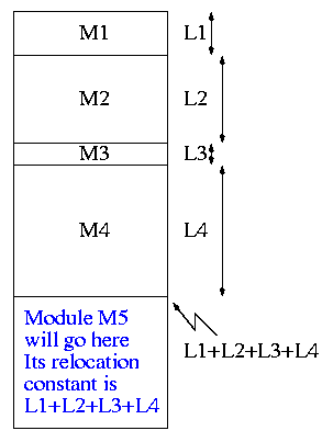
0.1.1 Relocating Relative Addresses
The compiler and assembler treat each module as if it will be
loaded at location zero.
For example, the machine instruction jump
120 is used to indicate a jump to location 120 of the
current module.
To convert this relative address to an
absolute address, the linker adds the
base address of the module to the relative address.
The base address is the address at which this module will be
loaded.
For example, assume a module is to be loaded starting at location
2300 and contains the above instruction jump 120
The linker changes this instruction to jump 2420
How does the linker know that the module is to be loaded starting
at location 2300?
It processes the modules one at a time.
(We assume) the first module is to be loaded at location zero.
So relocating the first module is trivial (adding zero).
We say that the relocation constant is zero.
After processing the first module, the linker knows its length
(say that length is L1).
Hence the second module is to be loaded starting at L1, i.e.,
the relocation constant is L1.
In general, the linker keeps the sum of the lengths of
all the modules it has already processed; this sum is the
relocation constant for the next module.
0.1.2 Resolving External References
If a C (or Java, or Pascal, or Ada, etc) module contains a function
call f(x) to a function f()
that is defined in a different module, the object
module containing the call must contain some kind of jump to the
beginning of f().
But this is impossible!
When the program is compiled, the compiler and assembler
do not see the definition of f() so there is
no way they can supply the starting address.
Instead a dummy address is supplied and a notation made that
this address needs to be filled in with the location of
f().
This is called a use of f().
The object module containing the definition
of f() contains a notation that f() is being
defined and gives the relative address of the definition, which
the linker converts to an absolute address (as above).
The linker then changes all uses of f() to the correct
absolute address.
0.1.3 An Example from Lab 1
To see how a linker works lets consider the following example,
which is the first dataset from lab #1.
The description in lab1 is more detailed.
The target machine is word addressable and each word consists of 4
decimal digits.
The first (leftmost) digit is the opcode and the remaining three
digits form an address.
The input begins with a positive integer giving the number of
object modules present.
Each object module contains three parts, a definition list, a use
list, and the program text itself.
The definition list consists of a count N followed
by N definitions.
Each definition is a pair (sym, loc)
signifying that sym is defined
at relative address loc.
The use list consists of a count N followed by N uses.
Each use is again a pair (sym, loc), but this time
signifying that sym is used in the linked
list started at loc.
The address initially in loc points to the next use of sym.
An address of 777 is the sentinel ending the list.
The program text consists of a count N followed
by N pairs (type, word),
where word is a 4-digit instruction as described above
and type is a single character indicating if the address in
the word is
Immediate,
Absolute,
Relative, or
External.
The actions taken by the linker depend on the type of the
address, as we now illustrate.
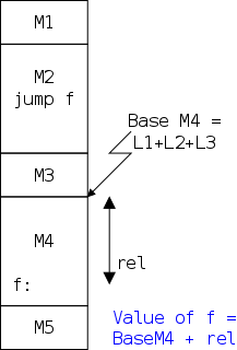
Consider the first input set from the lab.
  4
  1 xy 2
  2 xy 4 z 2
  5 R 1004  I 5678  E 2777  R 8002  E 7777
  0
  1 z 3
  6 R 8001  E 1777  E 1001  E 3002  R 1002  A 1010
  0
  1 z 1
  2 R 5001  E 4777
  1 z 2
  1 xy 2
  3 A 8000  E 1777  E 2001
The first pass simply finds the base address of each module and
produces the symbol table giving the values for xy and z (2 and 15
respectively).
The second pass does the real work using the symbol table and base
addresses produced in pass one.
The resulting output (shown below) is more detailed than I expect
you to produce.
The detail is there to help me explain what the linker is doing.
All I would expect from you is the symbol table and the rightmost
column of the memory map.
  Symbol Table
    xy=2
    z=15
  Memory Map
  +0
  0:       R 1004      1004+0 = 1004
  1:       I 5678               5678
  2: xy:   E 2777 ->z           2015
  3:       R 8002      8002+0 = 8002
  4:       E 7777 ->xy          7002
  +5
  0        R 8001      8001+5 = 8006
  1        E 1777 ->z           1015
  2        E 1001 ->z           1015
  3        E 3002 ->z           3015
  4        R 1002      1002+5 = 1007
  5        A 1010               1010
  +11
  0        R 5001      5001+11= 5012
  1        E 4000 ->z           4015
  +13
  0        A 8000               8000
  1        E 1777 ->xy          1002
  2 z:     E 2001 ->xy          2002
Note: It is faster (less I/O)
to do a one pass approach, but is harder since you need
fix-up code whenever a use occurs in a module that precedes
the module with the definition.
Note: The linker was originally called
a linkage editor by IBM.
Historical note: The linker on Unix was mistakenly called ld (for
loader), which is unfortunate since it links but does not
load.
Unix was originally developed at Bell Labs; the seventh edition
of Unix was made publicly available (perhaps earlier ones were
somewhat available).
The 7th ed man page for ld begins (see
https://cm.bell-labs.com/7thEdMan).
    .TH LD 1
    .SH NAME
    ld \- loader
    .SH SYNOPSIS
    .B ld
    [ option ] file ...
    .SH DESCRIPTION
    .I Ld
    combines several
    object programs into one, resolves external
    references, and searches libraries.
By the mid 80s the Berkeley version (4.3BSD) man
page referred to ld as link editor and this more accurate
name is now standard in Unix/Linux distributions.
During the 2004-05 fall semester a student wrote to me:
BTW - I have meant to tell you that I know the lady who wrote ld.
She told me that they called it loader, because they just really
didn't have a good idea of what it was going to be at the time.
Lab #1: Implement a two-pass linker.
See the class home page and NYU Brightspace for details.
Chapter 1 Introduction
Levels of abstraction (virtual machines)
Software is often implemented in layers (so is hardware, but that
is not the subject of this course).
The higher layers use the facilities provided by lower layers.
Alternatively said, the upper layers are written using a more
powerful and more abstract virtual machine than the lower layers.
In yet other words, each layer is written as though it runs on the
virtual machine supplied by the lower layers and in turn provides a
more abstract (pleasant) virtual machine for the higher layers to
run on.
Using a broad brush, the layers are.
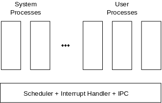
Applications (e.g., web browser) and utilities (e.g., compiler,
linker).
User interface (UI).
The UI may be text oriented (Unix/Linux shell, MS Windows Command,
MacOS Terminal) or graphical (GUI, e.g., MS Windows, Linux KDE,
MacOS).
Libraries (e.g., libc).
The OS proper (the kernel).
Hardware.
An important distinction is that the kernel runs in
privileged mode (a.k.a supervisor
mode or kernel mode); Whereas your programs, as
well as compilers, editors, shell, linkers, browsers, etc. run
in user mode.
Wnen running in supervisor mode a program is able to execute all
possible instructions.
In contrast, user-mode programs cannot directly execute I/O
instructions since such instructions are normally privileged.
So the programs you and I write cannot perform I/O;
but they can (and do) ask the OS to perform I/O for them.
The kernel is itself normally layered, e.g.
(Machine independent) files and filesystems.
(Machine independent) I/O.
(Machine dependent) device drivers.
The machine independent I/O layer is written assuming
virtual (i.e. idealized) hardware.
For example, the machine independent I/O portion can access a
certain byte in a given file.
In reality, I/O devices, e.g., disks, have no support or knowledge
of files; these devices support only blocks.
Lower levels of the software implement files in terms of blocks.
Often the machine independent part is itself more than one
layer.
The term Operating System is not well defined.
Is it just the kernel, i.e., the portion run in supervisor mode?
How about the libraries?
The utilities?
All these are certainly system software but it is
not clear how much is part of the OS.
1.1 What is an operating system?
As mentioned above, the OS raises the abstraction level by
providing a higher level virtual machine.
A second (related) major objective for the OS is to manage the
resources provided by this virtual machine.
1.1.1 The Operating System as an Extended Machine
The kernel itself raises the level of abstraction and hides
details.
For example a user (of the kernel) can write() to a file (a
concept not present in hardware) and can do so without knowing
whether the file resides on a solid-state-disk (SSD), an internal
SCSI disk, or an external server in Europe.
The user can also ignore issues such as whether the file is stored
contiguously or is broken into blocks.
Well designed abstractions are a key to managing complexity.
1.1.2 The Operating System as a Resource Manager
The kernel must manage the resources to handle contention and
resolve conflicts between users.
Note that by users, I am not referring directly to humans, but
instead to (user-mode) processes running on behalf of human
users.
Often the resource is shared or multiplexed among
the users.
This can take the form of time-multiplexing, where the
users take turns (e.g., the processor resource)
or space-multiplexing, where each user gets a part of the
resource (e.g., a disk drive).
With sharing comes various issues such as protection, privacy,
fairness, etc.
Question: How is an OS Fundamentally Different from (say) a Compiler?
Answer: Concurrency!
Per Brinch Hansen in Operating Systems Principles
(Prentice Hall, 1973) writes.
The main difficulty of multiprogramming is that concurrent activities
can interact in a time-dependent manner, which makes it practically
impossibly to locate programming errors by systematic testing.
Perhaps, more than anything else, this explains the difficulty of
making operating systems reliable.
Homework: 1.
What are the two main functions of an operating system?
(Unless otherwise stated, problems numbers are from the end of the
current chapter in the fourth edition of Tanenbaum.
For most problems, including this one, I have copied the problem
statement into the notes in case you have a different edition of
the book.)
1.2 History of Operating Systems
The subsection headings describe the hardware as well as the OS; we
are naturally more interested in the latter.
These two development paths are related since the improving hardware
enabled the more advanced OS features.
1.2.1 The first Generation (1945-55): Vacuum Tubes (and No OS)
One user (program; perhaps several humans) at a time.
Any operating-system-like functionality that was needed was part of
the user's program.
Although this time frame predates my own usage, computers without
serious operating systems existed during the second generation and
were then available to a wider (but still very select) audience.
I have fond memories of the Bendix G-15 (paper
tape) and the IBM 1620 (cards; typewriter; decimal).
During the short time you had the machine, it was truly a personal
computer.
1.2.2 The Second Generation (1955-65): Transitors and Batch Systems
Many jobs were batched together, but the systems were
still uniprogrammed, a job once started was run to
completion without interruption and then flushed from the system.
A change from the previous generation is that the OS was not
reloaded for each job and hence needed to be protected from the
user's execution.
As mentioned above, in the first generation, the beginning of a job
contained the trivial OS-like support features used.
Batches of user jobs were prepared offline (cards to magnetic
tape) using a separate computer (an IBM 1401 with a 1402 card
reader/punch).
The tape was brought to the main computer (an IBM 7090/7094) where
the output to be printed was written on another tape.
This tape went back to the service machine (1401) and was printed
(on a 1403).
1.2.3 The Third Generation (1965-1980): ICs and Multiprogramming
In my opinion multiprogramming was the biggest change to have
occurred from the OS point of view.
It is with multiprogramming (many processes executing concurrently)
that we have the operating system fielding requests whose arrival
order is non-deterministic.
At this point operating systems become notoriously hard to get right
due to the inability to test a significant percentage of the
possible interactions and the inability to reproduce bugs on
request.
Since multiple jobs are in memory at the same jobs, one job's
memory must be protected from the other jobs.
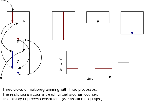
The Purpose of Multiprogramming
The purpose of multiprogramming is to overlap CPU and I/O activity
and thus greatly improve CPU utilization.
Recall that, during this time period, computers, in particular the
processors, were very expensive.
Multiple Batch Streams
IBM OS/MFT (Multiprogramming with a Fixed
number of Tasks).
An early OS for the IBM system 360.
Physical memory is partitioned at boot time and the size of
each partition cannot be changed until the system
reboots.
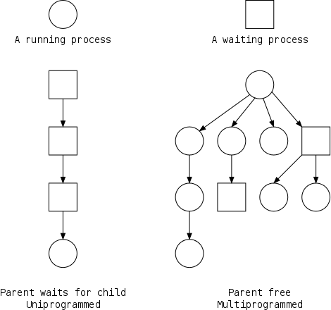
A batch of jobs is assigned to a each partition.
This batch is UNIprogrammed.
That is, the first job in the batch is loaded into the
partition and begins to execute.
The remainder of the batch waits for the first job to finish
and which point the second job in the batch is loaded and
runs.
Jobs residing in separate partitions are
MULTIprogrammed.
Specifically, when a job residing in one partition starts a
(slow) I/O, the CPU switches to executing the job loaded in
another partition.
Jobs were spooled from cards into the
memory; similarly output was spooled from the memory to
a printer.
More details are presented later, when we study memory
management.
IBM OS/MVT (Multiprogramming with a
Variable number of Tasks) (then other names).
Each job gets just the amount of memory it needs.
That is, the partitioning of memory changes as jobs
enter and leave.
Indeed, the memory used by a job can grow and shrink
dynamically (i.e., while the program is running).
MVT is a more efficient user of
resources, but is more difficult to implement.
Later, when we study OS/MVT in more detail, we will see
that, with varying size partitions, memory questions such as
compaction, holes, and fragmentation
arise.
Spooling
With multiprogramming, the offline preparation of job batches, as
done in the second generation, was no longer needed.
Instead one job could be loading (from say cards), another job could
be printing, and a third computing, all on the same computer.
So when a card deck was submitted by the user it could be read
directly into an on-disk queue on the main computer.
Then when the system is ready to run another job, it is already
there.
Similarly, jobs would print to disk and later another task
would really print these disk files onto paper.
This technique of reading and writing online fast storage while the
job is running and accessing the the slower devices separately is
often called spooling.
Time-Sharing
This is multiprogramming with rapid switching between jobs
(processes) so that, to the user it appears that their job is always
running (but at a slower rate than if run alone).
Also individual users spool their own printed output onto a
remote terminal.
Deciding when to switch and to which process to switch is
called scheduling.
We will study scheduling when we cover processor management a few
weeks from now.
MIT and Dartmouth were pioneers in time-sharing.
Since I went to MIT, I naturally believe MIT was first.
In particular, during my second semester (jan-may 1964), I took a
course that by luck was chosen to the first one on the MIT
timesharing system CTSS.
I do believe that I was in the first group of undergraduates (about
15 or 20 students I guess) to use time-sharing.
Tanenbaum also asserts that MIT was first, but again he was a
student there (in physics).
Homework:
What is multiprogramming?
Why was timesharing not widespread on second generation
computers?
What is spooling?
Do you think that advanced personal computers will have spooling
as a standard feature in the future?
5.
On early computers, every byte of data read or written was
handled by the CPU (i.e., there was no DMA).
What implications does this have for multiprogramming?
1.2.4 The Fourth Generation (1980-Present): Personal Computers
Serious PC Operating systems such as Unix/Linux, Windows
NT/2000/XP/Vista/10/etc and MacOS are now all multiprogrammed.
GUIs have become important.
What is not clear is whether the GUI should be part of the kernel,
or a separate layer on top of the kernel.
The Windows GUI is built in to the kernel, the MacOS and Linux GUIs
are separate layers.
Early PC operating systems were uniprogrammed and
their direct descendants lasted for quite some time (e.g., Windows
ME).
1.2.5 The Fifth Generation (1990-Present): Mobile Computers
Primarily hardware (and gui) changes.
Note: I very much recommend reading all of 1.2,
not for this course especially, but for general interest.
Tanenbaum writes well and is my age so lived through much of the
history himself.
Start Lecture #02
1.3 Computer Hardware Review
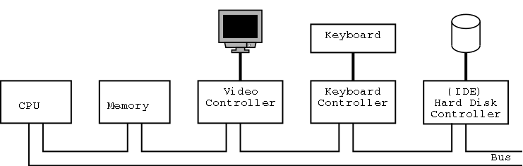
The picture above is very simplified; it represents a 1980 design.
(For one thing, today separate buses are used to Memory and
Video.)
A bus is a set of wires that connect two or more
devices.
Only one message can be on the bus at a time.
All the devices receive the message: There are no switches in
between to steer the message to the desired destination, but often
some of the wires form an address that indicates which devices
should actually process the message.
1.3.1 Processors
Only at a few points will we need to
understand the various processor registers such as the
program counter (a.k.a, instruction pointer), the
stack pointer, and the Program Status Words
(PSWs).
We will ignore computer design issues such as pipelining
and superscalar.
Many of these issues are mentioned in 201 and nearly all of them
are covered in 436, the computer architecture elective.
We do, however, need the notion of a trap, which
is an instruction that atomically switches the processor
into privileged mode and jumps to a pre-defined physical address.
This is the key mechanism for implementing system calls in
which a user program enters the operating system.
We will have much more to say about traps at the end of this chapter
and again later in the course.
Multithreaded and Multicore Chips
Many of the OS issues introduced by multi-processors of any flavor
are also found in a uni-processor, multi-programmed system.
In particular, successfully handling the concurrency offered by the
second class of systems, goes a long way toward preparing for the
first class.
The remaining multi-processor issues are not covered in this
course.
1.3.2 Memory
We will ignore caches (which are covered in 201 and 436; you can
see my online class notes, if you are interested), but we will later
discuss demand paging, which is similar in principle.
In both cases, the goal is to combine large, slow memory with small,
fast memory to achieve the effect of large, fast memory.
Despite their similarity, demand paging and
caches use largely disjoint terminology.
The central memory in a system is called RAM
(Random Access Memory).
A key point is that RAM is volatile, i.e. the memory loses its data
if power is turned off.
Hence when power is turned back on, the RAM contains junk.
Thus the first instructions executed at power-on cannot come from
RAM.
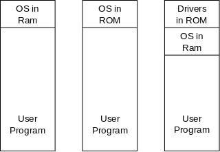
ROM / PROM / EPROM / EEPROM / Flash Ram
ROM (Read Only Memory) is used for (low-level
control) software that often comes with devices on general purpose
computers, and for the entire software system on
non-user-programmable devices such as microwaves and dumb
wristwatches.
It is also used for non-changing data.
A modern, familiar ROM is CD-ROM (or the denser DVD, or the even
denser Blu-ray).
ROM is non-volatile.
As a result, when a computer is turned on the first instructions
to be executed are from ROM.
But often this unchangable data needs to be changed (e.g., to fix
bugs).
This gives rise first to PROM (Programmable ROM),
which, like a CD-R, can be written once (as opposed to being mass
produced already written like a CD-ROM), and then
to EPROM (Erasable PROM), which is like a CD-RW.
Early EPROMs needed UV light for erasure;
EEPROM, Electrically EPROM or
Flash RAM) can be erased by normal circuitry, which
is much more convenient.
Memory Protection and Context Switching
As mentioned above when discussing
OS/MFT and OS/MVT, multiprogramming
requires that we protect one process from another.
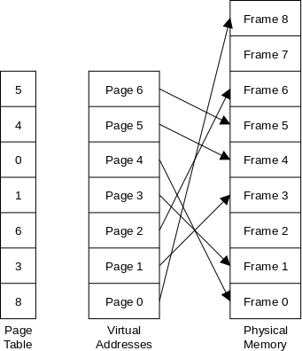
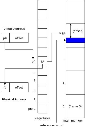
That is, we need to translate the virtual addresses
(a virtual address is the address as written in the program) into
physical addresses (a physical address is the
actual memory address in the computer) such that, at any
point in time, the physical address of each process are disjoint.
The hardware that performs this translation is called the
MMU or Memory Management Unit.
(There are special occasions when two
processes wish to share memory.)
Note the similarity between (1) translating
virtual to physical addresses by the OS and (2) relocating relative
addresses (into absolute addresses) in your lab 1 linker.
When context switching from one process to
another, the virtual-to-physical address translation must change,
which can be an expensive operation.
1.3.3 Disks
When we do I/O for real, I will show a real disk opened up and
illustrate the components
Platter
Surface
Head
Track
Sector
Cylinder
Seek time
Rotational latency
Transfer time
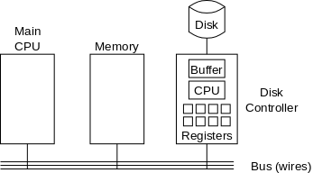
Devices are quite varied and often difficult to manage.
As a result a separate computer, called a controller, is used to
translate OS commands into what the device requires.
Solid State Disks (SSDs)
This is flash RAM organized in sector-like blocks as is a disk.
Unlike RAM, SSD is non volatile; unlike a disk it has no moving
parts (and hence is much faster).
The blocks can be written a large number of times.
However, the large number is not large enough to be
completely ignored.
1.3.A Tapes
At the bottom of the memory hierarchy we fine tapes, which have
large capacities, tiny cost per byte, and very long access times.
Tapes are becoming less important since their technology
improvement has not kept up with the improvement in disks.
We will not study tapes in this course.
1.3.4 I/O Devices
In addition to the disks and tapes just mentioned, I/O devices
include monitors (and their associated graphics controllers), NICs
(Network Interface Controllers), Modems, Keyboards, Mice, etc.
The OS communicates with the device controller, not with the device
itself.
For each different controller, a corresponding
device driver is included in the OS.
Note that, for example, many different graphics controllers are
capable of controlling a standard monitor, and hence the OS needs
many graphics device drivers.
In theory any SCSI (Small Computer System
Interconnect) controller can control any SCSI disk.
In practice this is not true as SCSI gets inproved to wide scsi,
ultra scsi, etc.
The newer controllers can still control the older disks and often
the newer disks can run in degraded mode with an older
controller.
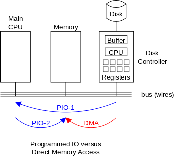
How Does the OS Know When I/O Is Complete?
Three methods are employed.
The OS can busy wait, constantly asking the
controller if the I/O is complete.
This is the easiest method, but can have low performance.
It is also called polling or
PIO (Programmed I/O).
The OS can tell the controller to start the I/O and then switch
to other tasks.
The controller must then interrupt the OS when
the I/O is done.
This method induces less waiting, but is harder to program
(concurrency!).
Moreover, on modern processors a single interrupt is rather
costly, much more costly than a single memory reference (but much,
much less costly than a disk I/O).
Some controllers can do
DMA (Direct Memory Access) in which case they
deal directly with memory after being started by the CPU.
A DMA controller relieves the CPU of some work and halves the
number of bus accesses.
We discuss these alternatives more in chapter 5.
In particular, we explain the last
point about halving bus accesses.
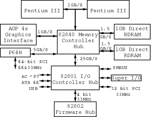
1.3.6 Buses
On the right is a figure showing the specifications for an Intel
chip set introduced in 2000.
The terminology used is not standardized, e.g., hubs are often
called bridges.
Most likely due to their location on the diagram to the right, the
Memory Controller Hub is often called the Northbridge and the I/O
Controller Hub the Southbridge.
As shown this chip set has two different width PCI
buses.
This particular chip set supplies USB.
An alternative is to have a PCI USB controller.
Unlike the situation in the previous diagram with a single bus, now
several pairs of components can be communicating simultaneously,
giving a significant improvement in performance (and
complexity).
1.3.7 Booting the Computer
When the power button is pressed, control starts at the BIOS, a
PROM (typically flash) in the system.
Control is then passed to (the tiny program stored in) the MBR
(Master Boot Record), which is the first 512-byte block on the
primary disk.
Control then proceeds to the first block in the active
partition and from there the OS is finally invoked (normally via an
OS loader).
Question: Since the power was turned off, why
doesn't the BIOS contain junk when the power is turned back
on? Answer: RAM is volatile, but ROM is not.
The above assumes that the boot medium selected by
the bios was the hard disk.
Other possibilities include a CD-ROM or the network.
1.4 OS Zoo
There is not much difference between mainframe, server,
multiprocessor, and PC OS's.
Indeed the 3e (third edtion) of Tannenbaum considerably softened the
differences given in the 2e and this softening continues in the 4e.
For example Unix/Linux and Windows run on all of above classes.
This course covers all four of those classes, which perhaps should
be considered just one class .
1.4.1 Mainframe Operating Systems
Used in data centers, these systems offer tremendous I/O
capabilities and extensive fault tolerance.
1.4.2 Server Operating Systems
Perhaps the most important servers today are web servers.
Again I/O (and network) performance are critical.
1.4.3 Multiprocessor Operating systems
A multiprocessor (as opposed to a multi-computer or multiple
computers or computer network or grid) means multiple processors
sharing memory and controlled by a single instance of the OS, which
typically can run on any of the processors.
Often it can run on several simultaneously.
Multiprocessors existed almost from the beginning of the computer
age, but now are not exotic.
Indeed, even my current laptop is a multiprocessor.
Multiple computers
The operating system(s) controlling a system of multiple
computers often are classified as either a Network OS or
a Distributed OS.
The former is basically a collection of ordinary PCs on a LAN that use
the network facilities available on PC operating systems.
Some extra utilities are often present to ease running jobs on
remote processors.
A Distributed OS is a more sophisticated
and seamless version of the above where the boundaries
between the processors are made nearly invisible to users (except
for performance).
This subject is not part of our course (but often is covered
in 2251).
1.4.4 PC Operating Systems
In the past some OS systems (e.g., ME) were claimed to be
tailored to client operation.
Others felt that they were restricted to client operation.
This seems to be gone now; a modern PC OS is fully functional.
I guess for marketing reasons some of the functionality can be
disabled.
1.4.5 Handheld Computer Operating Systems
This includes phones.
The only real difference between this class and the above is the
restriction to very modest memory and very low power.
However, the very modest memory keeps getting bigger and
some phones now include a stripped-down linux.
1.4.6 Embedded Operating Systems
The OS is part of the device, e.g., microwave ovens,
and cardiac monitors.
The OS is on a ROM so is not changed.
Since no user code is run, protection is not as important.
In that respect the OS is similar to the very earliest computers.
Embedded OS are very important commercially, but not covered much
in this course.
1.4.7 Sensor Node Operating Systems
These are embedded systems that also contain sensors and
communication devices so that the systems in an area can
cooperate.
1.4.8 Real-time Operating Systems
As the name suggests, time (more accurately timeliness) is an
important consideration.
There are two classes: soft vs hard real time.
In the latter, missing a deadline is a fatal error—sometimes
literally.
Very important commercially, but not covered much in this
course.
1.4.9 Smart Card Operating Systems
Very limited in power (both meanings of the word).
1.5 Operating System Concepts
This will be very brief.
Much of the rest of the course will consist of
filling in the details.
1.5.1 Processes
A process is program in execution.
If you run the same program twice, you have created two processes.
For example if you have two programs compiling in two windows, each
instance of the compiler is a separate process.
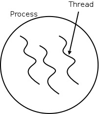
Often one distinguishes the state or context of a process—its
address space (roughly its memory image), open files,
etc.—from the thread of control.
If one has many threads running in the same task,
the result is a multithreaded processes.
The OS keeps information about all processes in the
process table.
Indeed, the OS views the process as the entry.
This is an example of an active entity (a process) being viewed as a
data structure (an entry in the process table), an observation I
first encountered in the (out of print) OS textbook by Finkel I
mentioned previously.
Discrete Event Simulations provide
another example of active entities being viewed as data
structures.
The data contained in a process table entry has many uses.
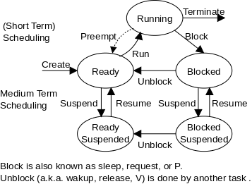
For example, it enables a processes that is currently preempted,
blocked, or suspended to resume execution in the future.
Another example is the entry containing the location of the current
directory, which enables a process to utilize relative address for
files.
Thanks to the OS each process can act as though it has the entire
CPU for itself and the entire memory for itself.
This is called virtualization.
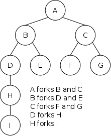
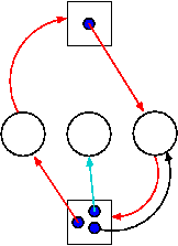
The Process Tree
The set of processes forms a tree via the (Unix) fork system call.
The forker is called the parent of the forkee,
which is called the child.
If the system always blocks the parent until the child finishes, the
tree is quite simple, just a line.
However, in modern OSes, the parent is free to continue executing
and in particular is free to fork again, thereby producing another
child, a sibling of the first child.
This produces a process tree as shown on the far right.
One process can send a signal to another process to
cause the latter to execute a predefined function (the signal
handler).
It can be tricky to write a program with a signal
handler since the programmer does not know at what point in
the mainline program the signal handler will be invoked.
Imagine writing two cooperating
programs f()
and g() knowing that, at some
undetermined point
of f(), the
program g() will be called.
Each user is assigned a User IDentification (UID)
and all processes created by that user have this UID.
A child has the same UID as its parent.
It is sometimes possible to change the UID of a running process.
A group of users can be formed and given a Group
IDentification, GID.
One UID is special (the superuser or
administrator) and has extra privileges.
Access to files and devices can be limited to a given UID or GID.
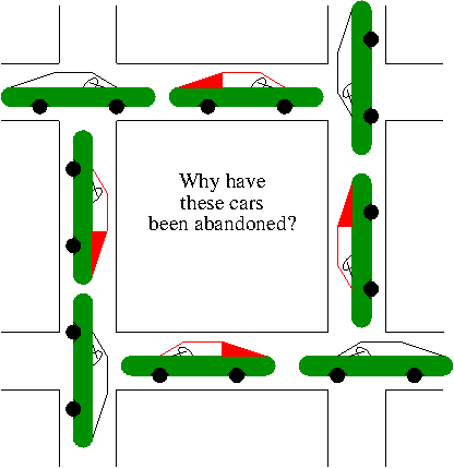
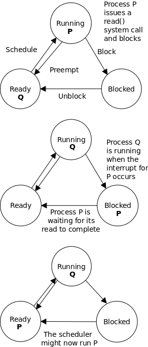
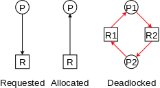
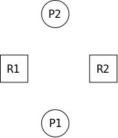
Deadlocks
A set of processes is deadlocked if each of the processes
is blocked by a process in the set.
The automotive equivalent, shown below, is called gridlock.
(The photograph was sent to me by Laurent Laor, a former 2250
student.)
1.5.2 Address Spaces
Clearly, each process requires memory, but there are other issues
as well.
For example, linkers produce a load module that assumes the process
is loaded at location 0.
The result is that every load module has the same (virtual) address
space.
The operating system must ensure that the virtual addresses of
concurrently executing processes are assigned disjoint physical
memory.
For another example note that current operating systems
permit each process to be given more
(virtual) memory than the total amount of
(real) memory on the machine.
1.5.3 Files
Modern systems have a hierarchy of files.
A file system tree.
In MSDOS the hierarchy is a forest not a tree.
There is no file, or directory that is an ancestor of both
a:\ and c:\.
In Unix all files are descendants of the root.
I suspect this is true of MacOS, which is Unix on the inside.
In recent versions of Windows, My Computerlooks like the parent of a:\ and c:\, but that is a feature
of the UI not the file systems.
In Unix the existence of (hard) links weakens the tree to a DAG
(directed acyclic graph).
Unix also has symbolic links, which when used indiscriminately,
permit directed cycles (i.e., the result is not a DAG).
Windows has shortcuts, which are somewhat similar to symbolic
links.
You can name a file via an absolute path starting
at the root directory (or in Windows A root
directory) or via a relative path starting at the
current working directory.
One requirement for this functionality is that the OS must know the
current working directory for each process.
As a result the operating system stores the location of the current
working directory in the process table entry for each process.
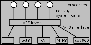
In addition to regular files and directories, Unix also uses the
file system namespace for devices (called
special files), which are typically found in
the /dev directory.
That is, in some ways you can treat the device as a file.
In particular some utilities that are normally applied to (ordinary)
files can be applied as well to some special files.
For example, when you are accessing a Unix system using a mouse,
type the following command cat /dev/mouse
and then move the mouse.
On my more modern system the command is cat /dev/input/mice
You kill the cat (sorry) by typing cntl-C.
I tried this on my linux box (using a text console) and no damage occurred.
Your mileage may vary.
Before a file can be accessed, it is
normally opened and a file descriptor obtained.
Subsequent I/O system calls (e.g., read and write) use the file
descriptor rather than the file name.
This is an optimization that enables the OS to find the file once
and save the information in a file table accessed by the file
descriptor.
Many systems have standard files that are automatically made
available to a process upon startup.
These (initial) file descriptors are fixed.
standard input: fd=0
standard output: fd=1
standard error: fd=2
A convenience offered by some command interpreters is a pipe or
pipeline.
For example the following command dir | wc -w
pipes the output of dir into a word counter.
The overall result is the number of files in the directory.
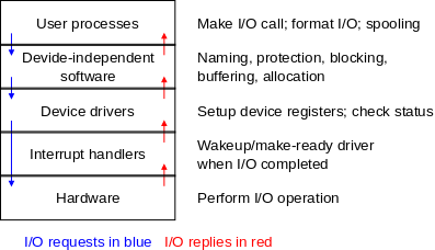
1.5.4 Input/Output
There are a wide variety of I/O devices that the OS must manage.
The OS contains device specific code (drivers) for each device
(really each controller) as well as device-independent I/O code.
Although all devices of a given type (e.g., disks) perform
essentially the same actions (e.g., read a block or write a block)
different devices require different commands and hence require
different drivers.
1.5.5 Protection
Files and directories have associated permissions.
Most systems supply at least rwx (readable, writable,
executable).
Separate permissions can be defined for the file's owner (files,
like processes and users, have UIDs and GIDs), for other users
with the same GID as the file, and for everyone else.
When a file is opened, permissions are checked and, if the
open is permitted, a file descriptor is returned that is used
for subsequent operations.
A more general mechanism is to provide an
access control list for each file.
Often files have attributes as well.
For example the linux ext2/3/4 file systems support a d
attribute that is a hint to the dump program not to backup this
file.
Memory assigned to a process, i.e., an address space, must be
protected so that unrelated processes do not read and write each
others' memory.
Security
Security has sadly become a very serious concern.
The topic is quite deep mathematically and I do not feel that the
necessarily superficial coverage that time would permit is useful
so we are not covering the topic at all.
1.5.6 The Shell (or Command Interpreter)
The shell presents the command line interface to the operating
system and offers several convenient features.
Invoke commands.
Pass arguments to the commands.
Redirect the output of a command to a file or device.
Redirect the input of a command to be from a file or device.
Pipe one command to another (as illustrated above via
dir | wc -w).
Instead of a shell, one can have a more graphical interface.
Homework: 12.
Which of the following instructions should be allowed only in kernel
mode?
Disable all interrupts.
Read the time-of-day clock.
Set the time-of-day clock.
Change the memory map.
1.5.7 Ontogeny Recapitulates Phylogeny
Some concepts become obsolete and then reemerge due in both cases
to technology changes.
Several examples follow.
Perhaps the cycle will repeat with smart card OS.
Large Memories (and Assembly Language)
The use of assembly languages greatly decreases when memories get
larger.
When minicomputers and microcomputers (early PCs) were first
introduced, they each had small memories and for a while assembly
language again became popular.
Protection Hardware (and Monoprogramming)
Multiprogramming requires protection hardware.
Once the hardware becomes available monoprogramming becomes obsolete.
Again when minicomputers and microcomputers were introduced, they had
no such hardware so monoprogramming revived.
Disks (and Flat File Systems)
When disks are small, they hold few files and a flat (single
directory) file system is adequate.
Once disks get large a hierarchical file system is necessary.
When mini and microcomputer were introduced, they had tiny disks and
the corresponding file systems were flat.
Virtual Memory (and Dynamically Linked Libraries)
Virtual memory, discussed in great detail later, permits
a single program to address more memory than present in the
computer (the latter is called physical memory).
The ability to dynamically remap address also permits programs to
link to libraries during runtime.
Hence, when VM hardware becomes available, so does dynamic
linking.
1.6 System Calls
A System call is the mechanism by which a user
(i.e., a process running in user mode) directly interfaces with the
OS.
Some textbooks use the term envelope for the component of
the OS responsible for fielding system calls
and dispatching them to the appropriate component of the
OS.
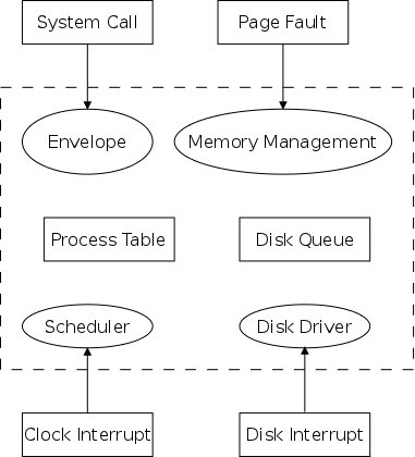
On the right is a picture showing some of the OS components and the
external events for which they are the interface.
Note that the OS serves two masters.
The hardware (at the bottom) asynchronously sends
interrupts and the user (at the top) synchronously invokes
system calls and generates page faults.
There is an important difference between these two cases.
When the user process issues a system call or generates a page
fault, it clearly must be running, which implies that the
operating system is not executing.
When the operating system last relinquished control, it had the
opportunity to prepare itself for processing a system call or a
page fault.
In contrast, at almost any point during execution,
including execution of most of the OS, an
interrupt can occur that will transfer control immediately to
certain points in the operating system (e.g., to a disk driver or
to the scheduler).
This means that at (almost) any point during its execution, the OS
must be prepared for an immediate transfer to a driver or the
scheduler.
Since the code being executed just prior to the interrupt might
well be OS code and hence might be using variables shared with the
drivers and the scheduler, writing the OS so that it is prepared
for this immediate transfer is not easy.
1.6.A Executing a System Call
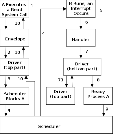
What happens when a user executes a system call such as read()?
I realize that it is unlikely you have ever directly issued a
read().
Instead, when you needed to read a file or the keyboard you would
have used the library routine scanf() if you are
programming in C or would have used the Scanner class
if you were programming in Java.
However, the C library routine scanf()
itself does issue
read() and so does the Scanner class.
A Method Call and the Runtime Stack
Before considering the read() system call, it might be
good to review a typical call/return sequence for a more familiar
situation, a method call in a high-level language.
On the right we see the assembler-like instructions that would
appear when a method invokes sin(x).
The numbers on the left represent memory locations.
For simplicity, we assume the machine is word addressable and
each instruction occupies one word.
The sin() method is in words 1042-1102 and the caller is
from 40-300.
We are interested in the call itself, which occupies 60-61.
The problems we need to solve are first to transfer control from
the caller to sin() passing the value of x and
second to transfer control back returning the calculated value
of sin(x).
The key data structure is a run-time stack whose changing contents
we will show on the board.
The first instruction (in word 60) pushes x onto the
stack.
Next we push the return address (which is 62) onto the stack and
jump to the sin routine.
The sin routine obtains x from the stack.
Now the sin() routines calculate sin(x) and puts the result in
register 1 (the assumed protocol for returning a value).
This code section might push and pop the stack many times but is
required to end with the stack in the same state as when the code
section began.
Specifically, the TopOfStack pointer will be restored
and the contents of the stack will be the same as it was
when sin() was jumped to.
We pop the stack obtaining the return address and jump to that
address.
We are now back in the caller, one instruction after the
call.
The caller pops x off the stack.
Note that now, after the call and return, the stack is back to the
state it had when we began.
The read() System Call
We show a detailed picture below, but at a high level, the following
actions occur.
A user program (in C, Java, etc.) makes a normal function call to
an I/O library routine (e.g., printf()).
The library routine (in C, or similar) does tasks
like formatting output and calls a small assembler routine.
The assembler routine moves
arguments to a predefined place and issues a trap.
The OS runs in
supervisor mode and performs the (possibly complex) actions
required.
The OS issues an RTI
(return-from-interrupt), which switches the system back to user
mode and returns to the assembly routine.
The assembly routine moves the
result to where the library routine expects it and returns to the
library routine.
The library routine does its remaining work and
then returns to the user program.
A typical invocation of the (Unix) read system call is:
count = read(fd,&buffer,nbytes)
This invocation reads up to nbytes from the file
specified by the file descriptor fd into the character
array buffer.
The actual number of bytes read is returned (it might be less than
nbytes if, for example, an end-of-file was encountered).
In more detail, the steps performed are as follows.
Push the third parameter on the stack.
Push the second parameter on the stack (the & is a
C-ism).
Push the first parameter on the stack.
Call the library routine, which involves saving the return
address and jumping to the routine, just like the call
to sin() above.
Machine/OS dependent actions, for example putting the system
call number corresponding to read() in a well defined
place, such as a specific register.
This may require assembly language.
Trap (a magic instruction) causes control to enter the operating
system proper and shifts the computer to privileged mode.
Assembly language is required.
The envelope uses the system call number to access a table of
pointers and finds the handler for read().
The read system call handler processes the request.
Another magic instruction (RTI) returns to user mode and jumps
to the location right after the trap.
The library routine returns (there is more; e.g., the count must
be returned).
The read() is done; can use the value read.
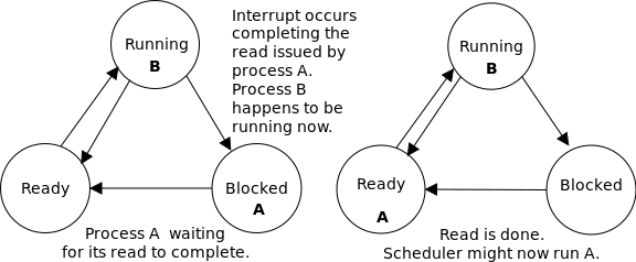
A major complication is that the system call handler may
block.
Indeed, the read system call handler is likely to block.
In that case the operating system will probably switch to another
process.
Such process switching is far from trivial and is discussed later in
the course.
1.6.A Table of Some System Calls
A Few Important Posix/Unix/Linux and Win32 System Calls
Posix
Win32
Description
Process Management
Fork
CreateProcess
Clone current process
exec(ve)
Replace current process
wait(pid)
WaitForSingleObject
Wait for a child to terminate.
exit
ExitProcess
Terminate process & return status
File Management
open
CreateFile
Open a file & return descriptor
close
CloseHandle
Close an open file
read
ReadFile
Read from file to buffer
write
WriteFile
Write from buffer to file
lseek
SetFilePointer
Move file pointer
stat
GetFileAttributesEx
Get status info
Directory and File System Management
mkdir
CreateDirectory
Create new directory
rmdir
RemoveDirectory
Remove empty directory
link
(none)
Create a directory entry
unlink
DeleteFile
Remove a directory entry
mount
(none)
Mount a file system
umount
(none)
Unmount a file system
Miscellaneous
chdir
SetCurrentDirectory
Change the current working directory
chmod
(none)
Change permissions on a file
kill
(none)
Send a signal to a process
time
GetLocalTime
Elapsed time since 1 jan 1970
1.6.1 System Calls for Process Management
We describe very briefly some of the Unix (Posix) system calls.
A short description of the Windows interface is in the book.
To show how the four process management calls in the table enable
much of process management, consider the following highly simplified
shell (the Unix command interpreter).
  while (true)
     display_prompt()
     read_command(command)
     if (fork() != 0)
        waitpid(...)
     else
        execve(command)
     endif
  endwhile
The fork() system call duplicates the process.
That is, we now have a second process, which is a child of the
process that actually executed the fork().
The parent and child are very, VERY nearly identical.
For example they have the same instructions, they have the same
data, and they are both currently executing the fork()
system call.
But there is a difference!
The fork() system call returns a zero in the child
process and returns a positive integer in the parent.
In fact the value returned to the parent is the PID (process ID) of
the child.
Thus, the parent and child execute different branches of the
if-then-else in the code above.
Note that simply removing the waitpid(...) lets the child continue
(in the background) while permits the user to start another
job.
1.6.2 System Calls for File Management
Most files are accessed sequentially from beginning to end.
In this case the operations performed are open() -- possibly creating
the file
multiple read()s and write()s close()
For non-sequential access, lseek is used to move
the File Pointer, which is the location in the file where the
next read or write will take place.
1.6.3 System Calls for Directory Management
Directories are created and destroyed by mkdir
and rmdir.
Directories are changed by the creation, modification, and deletion
of files.
As mentioned, open can create files.
Files can have several names: link gives another name to
an existing file and unlink removes a name.
When the last name is gone
(and the file is no longer open by any process)
, the file data is destroyed.
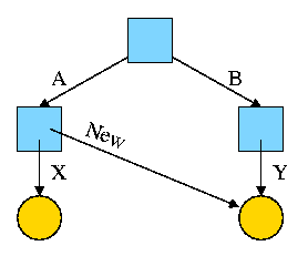
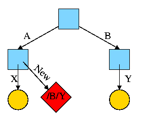
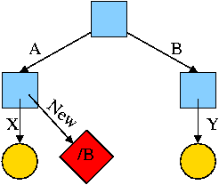
In Unix, one file system can be mounted on
(attached to) another.
When this is done, access to an existing directory on the second
filesystem is temporarily replaced by the entire first file system.
Most often the directory chosen is empty before the mount so no
files become (temporarily) invisible.
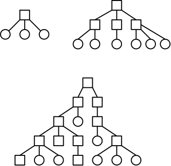
The top picture shows two file systems; the second row shows the
result when the right-hand file system is mounted on /y.
In both cases squares represent directories and circles represent
regular files.
This is how a Unix system enables all files, even those on
different physical disks and using different filesystems, to be
descendants of a single root
1.6.4 Miscellaneous System Calls
1.6.5 The Windows Win32 API
Homework: For each of
the following system calls, give a condition that causes it to
fail: fork, exec,
and unlink.
1.A Addendum on Transfer of Control
The transfer of control between user processes and the operating
system kernel can be quite complicated, especially in the case of
blocking system calls, hardware interrupts, and page faults.
We tackle these issues later; here we examine the familiar example
of a procedure call within a user-mode process.
An important OS objective is that, even in the more complicated
cases of page faults and blocking system calls requiring device
interrupts, simple procedure call semantics are observed
from a user process viewpoint.
The complexity is hidden inside the kernel itself, yet another example
of the operating system providing a more abstract, i.e., simpler,
virtual machine to the user processes.
More details will be added when we study memory management (and
know officially about page faults) and more again when we study I/O
(and know officially about device interrupts).
A number of the details below are far from standardized.
Such items as where to place parameters, which routine saves the
registers, exact semantics of trap, etc, vary as one changes
language/compiler/OS.
Indeed some of these are referred to as calling conventions,
i.e. their implementation is a matter of convention rather then
logical requirement.
The presentation below is, I hope, reasonable, but must be viewed
as a generic description of what could happen, rather then a real
description of what does happen with, say, C compiled by the
Microsoft compiler running on Windows 10.
1.A.1 User-mode Procedure Calls
Procedure f calls g(a,b,c) in process P.
An example is above where a user program calls
read(fd,buffer,nbytes).
Note that both f() and g() are in the same
process P and no action goes outside P.
Thus we will not mention the process again in this description.
Actions by f Prior to the Call
Save the registers by pushing them onto the stack.
(In some implementations this is done by
g
instead of by
f
or by
g and
f combined
).
Push arguments c,b,a onto the stack.
Note: These stacks usually grow downward, so
pushing an item onto the stack actually involves decrementing the
stack pointer, SP.
Note: Some systems store arguments in registers
not on the stack. Question: Why are the parameters pushed in
reverse order? Hint: How many parameters
does printf() take?
Executing the Call Itself
Execute METHODCALL <start-address of g>.
This instruction saves the program counter, PC
(a.k.a. the instruction pointer, IP), and jumps to the start
address of g.
The value saved is actually the updated program counter, i.e.,
the location of the next instruction (the instruction of f to be
executed when g returns).
Actions by g Upon Being Called
Allocate space for g's local variables by
suitably decrementing SP.
Start execution from the beginning of g, referencing the
parameters as needed.
The execution may involve calling other procedures, possibly
including recursive calls to f and/or g.
Actions by g When Returning to f
If g is to return a value, store it in the conventional
place.
Undo step 4: Deallocate local variables
by suitably incrementing SP.
Undo step 3: Execute a RETURN instruction, setting PC
to the return address saved in step 3.
Actions by f Upon the Return from g:
(We are now at the instruction in f immediately following the
call to g.)
Undo step 2: Remove the arguments from the
stack by suitably incrementing SP.
Undo step 1: Restore the registers while popping their values off the
stack.
Continue the execution of f, referencing the returned value of g,
if any.
Properties of (User-Mode) Procedure Calls
Predictable (often called synchronous) behavior: The author of f
knows where and hence when the call to g will occur.
There are no surprises, so it is relatively easy for the
programmer to ensure that f is prepared for the transfer of
control.
LIFO (stack-like) transfer of control: we can be sure
that control will return to f() when the call
to g() exits.
The above statement holds even if g()
calls h() and then h() calls d().
In fact it even holds if, via recursion, g()
calls f().
We are ignoring language features such as
throwing and catching exceptions, and the use of
unstructured assembly coding.
In these cases all bets are off.
Everything happens entirely in user mode and user space.
1.A.2 Kernel-mode Procedure Calls
We now consider one procedure running in kernel mode calling
another procedure, which also runs in kernel mode, i.e., a procedure
call within the operating system itself.
In the next section, we will discuss switching from user mode to
kernel mode and back.
There is not much difference between the actions taken during a
kernel-mode procedure call and during a user-mode procedure call.
The procedures executing in kernel-mode are permitted to issue
privileged instructions, but the instructions used for transferring
control are all unprivileged so there is no change in that
respect.
One difference is that often a different stack is
used in kernel mode, but that simply means that the stack pointer
must be set to the kernel stack when switching from user to kernel
mode.
But we are not switching modes in this section; the stack pointer
already points to the kernel stack.
Often there are two stack pointers one for kernel mode and one for
user mode.
Start Lecture #04
1.A.3 The Trap/RTI Instructions: Switching Between User
and Kernel Mode
The trap instruction, like a procedure call, is a synchronous
transfer of control: We can see where, and hence when, it is
executed.
In this respect, there are no surprises.
Although not surprising, the trap instruction does have an unusual
effect: processor execution is switched from user-mode to
kernel-mode.
That is, the trap instruction normally is itself executed in
user-mode (it is naturally an UNprivileged instruction), but
the next instruction executed (which is NOT the instruction
written after the trap) is executed in kernel-mode.
Process P, running in unprivileged (user) mode, executes a trap.
The code being executed is written in assembler since there are no
high level languages that generate a trap instruction.
There is no need for us to name the function that is executing.
Compare the following example to the explanation of f calls g
given above.
Actions by P prior to the trap
Save the registers by pushing them onto the stack.
Store any arguments that are to be passed.
The stack is not normally used to store
these arguments since the kernel has a different stack.
Often registers are used.
Executing the trap itself
Execute TRAP <trap-number>.
This instruction switch the processor to kernel (privileged) mode,
jumps to a location in the OS determined by trap-number, and saves
the return address.
For example, the processor may be designed so that the next
instruction executed after a trap is at physical address 8 times
the trap-number.
(The trap-number can be thought of as the name of the
code-sequence to which the processor will jump rather then as an
argument to trap.)
Actions by the OS upon being TRAPped into
Jump to the real code.
Recall that trap instructions with different trap numbers jump to
locations very close to each other.
There is not enough room between them for the real trap handler.
Indeed one can think of the trap as having an extra level of
indirection; it jumps to a location that then jumps to the real
start address.
If you remember using assembler jump tables in 201 to
implement switch statements, this is very
similar.
Check all the arguments passed.
The kernel must be paranoid and assume that the authors of the
user mode program wear black hats.
Allocate space by decrementing the kernel stack pointer.
The kernel and user stacks are usually separate.
Start execution from the jumped-to location.
Actions by the OS when returning to user mode
If a value is to be returned, store it in the conventional
place.
Undo step 6: Deallocate space by incrementing the kernel stack
pointer.
Undo step 3: Execute (in assembler) another special instruction,
RTI or ReTurn from Interrupt, which returns the processor to user
mode and transfers control to the return location saved by the
trap.
The word interrupt appears because an RTI is also used when
the kernel is returning from an interrupt as well as the present
case when it is returning from a trap.
Actually, an RTI doesn't always go back to
user mode.
Instead it returns to the mode in effect before the trap or
interrupt.
Actions by P upon the return from the OS
We are now in at the instruction right after the trap Undo
step 2: Reclaim any space used by the arguments.
Undo step 1: Restore the registers by popping the
stack.
Continue the execution of P, referencing the returned value(s)
of the trap, if any.
Properties of TRAP/RTI
Synchronous behavior: The author of the assembly code in P knows
where and hence when the trap will occur.
There are no surprises, so it is relatively easy for the
programmer to prepare for the transfer of control.
Trivial control transfer when viewed from P: The next
instruction of P that will be executed is the one
following the trap.
As we shall see later, other processes may execute between P's
trap instruction and P's next instruction.
Starts and ends in user mode and user space, but executed in
kernel mode and kernel space in the middle.
Note:
A good way to use the material in the addendum is to compare the first
case (user-mode f calls user-mode g) to the TRAP/RTI case line by line
so that you can see the similarities and differences.
Start Lecture #03
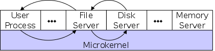
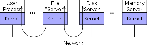
1.7 Operating System Structure
I must note that Tanenbaum is a strong advocate of the so called
microkernel approach in which as much as possible is moved out of
the (supervisor mode) kernel into separate (user-mode) processes
(I recommend his article in CACM March 2016).
The (hopefully small) portion left in supervisor mode is called a
microkernel.
In the early 90s this was popular.
Digital Unix (subsequently called True64) and Windows NT were
microkernel based.
Digital Unix was based on Mach, a research OS from Carnegie Mellon
university.
However, for performance reasons, subsequent versions of Windows
were hybrid designs as was OS X for the Mac (see Tanenbaum CACM
article referenced above).
Lately, the growing popularity of Linux has called into
question the once-felt belief that
all new operating systems will be microkernel based.
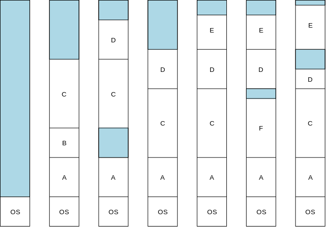
The system switches from user mode to kernel mode during the trap
and then back when the OS does an RTI (return from interrupt).
While in supervisor mode, the OS naturally includes procedure
calls and returns.
Modern monolithic systems, such as Linux, are not
completely monolithic in that during execution, they can load code
modules as needed.
This load on demand capability is mainly used for device
drivers.
We can structure the system better than above might suggest, which
brings us to ...
1.7.2 Layered Systems
Some systems have more layers than shown on the right and are more
strictly structured.
An early layered system was THE operating system by
Dijkstra and his students at Technische Hogeschool Eindhoven.
This was a simple batch system so the operator was the user.
The layering was done by convention, i.e. there was no enforcement
by hardware and the entire OS was linked together as one program.
This is true of many modern OS systems as well (e.g., linux).
The actual layers were
The operator process
User programs
I/O mgt
Operator console—process communication
Memory and drum management
The MULTICS system was layered in a more formal manner.
The (specialized) hardware provided several protection layers and
the OS used them.
That is, arbitrary OS code could not jump into or access data in a
more protected layer.
1.7.3 Microkernels
The idea is to have the kernel, i.e. the portion running in
supervisor mode, as small as possible and to have most of the
operating system functionality provided by separate processes.
The microkernel provides just enough to implement
processes.
This has significant advantages.
For example an error in the file server cannot corrupt memory in the
process server since they have separate address spaces (they are
after all separate process).
Confining the effect of errors makes them easier to track down.
Also an error in the ethernet driver can corrupt or stop network
communication, but it cannot crash the system as a whole.
However, the microkernel approach does mean that when a (real) user
process makes a system call there are more processes switches.
These are expensive and have hindered the adoption of pure
microkernel operating systems.
Related to microkernels is the idea of putting
the mechanism in the kernel, but not the policy.
For example, the kernel would know how to select the highest
priority process and run it, but some external process would assign
the priorities.
In this way changing the priority scheme could become a relatively
minor event compared to the situation in monolithic systems where
the entire kernel must be relinked and rebooted.
Microkernels Not So Different In Practice
The following quote is from a February 2012 interview of Dennis
Ritchie, the inventor of the C programming language and co-inventor,
with Ken Thompson, of Unix.
What's your opinion on microkernels vs. monolithic?
They're not all that different when you actually use them.
Micro kernels tend to be pretty large these days,
monolithic kernels with loadable device drivers are taking up
more of the advantages claimed for microkernels.
I should note, however, that Tanenbaum's Minix microkernel
(excluding the processes) is quite small, about 13,000
lines.
1.7.4 Client-Server
When implemented on one computer, a client-server OS often uses the
microkernel approach shown above in which the microkernel just handles
communication between clients and servers, and the main OS functions
are provided by a number of separate processes.
A distributed system can be thought of as an extension of the
client server concept where the servers are remote.
The figure on the right would describe a distributed system of
yesteryear, where memory was scarce and it would be considered
lavish to have full systems on each machine.
Today with plentiful memory, each machine would have all the
standard servers and specific servers for every device on that
system.
So the only reason an OS-internal message would be sent to a remote
computer RC, is if the originating process wished to communicate with
a specific process running on RC or a specific device attached to
RC.
Distributed systems are becoming increasingly
important for application programs.
Perhaps the program needs data found only on certain machine (no one
machine has all the data).
For example, think of (legal, of course) file sharing
programs.
Distributed systems are also used to reduce the time required by an
application.
You do this by dividing the program into pieces, which are run
concurrently on separate computers.
Homework:
The client-server model is popular in distributed systems.
Can it also be used in single-computer system?
1.7.5 Virtual Machines
The idea is to use a hypervisor (i.e., beyond a supervisor,
i.e. beyond a normal OS) to switch between multiple
Operating Systems.
The modern name for a hypervisor is a
Virtual Machine Monitor (VMM).
VM/370
The hypervisor idea was made popular by IBM's CP/CMS (now VM/370).
CMS stood for Cambridge Monitor System since it was developed at
IBM's Cambridge (MA) Science Center.
It was renamed, with the same acronym (an IBM specialty, cf. RAID)
to Conversational Monitor System.
Each App/CMS runs on a virtual 370.
CMS is a single user OS.
A system call in an App (application) traps to the
corresponding CMS.
CMS believes it is running on the actual hardware so issues I/O
instructions but ...
... I/O instructions in CMS trap to VM/370.
This idea is still used but the guest OS is now normally a
full-featured operating system rather then a simple system like
CMS.
For example, the newest IBM systems can run multiple instances
of linux as well as multiple instances of traditional IBM
Operating Systems on a single hardware platform.
Virtual Machines Redicovered
Recently, virtual machine technology has moved to machines (notably
x86) that are not fully virtualizable.
Recall that when CMS executed a privileged instruction, the hardware
trapped to the real operating system.
On x86, privileged instructions are ignored when executed
in user mode, so running the guest OS in user mode won't work.
Bye bye (traditional) hypervisor.
But a new style emerged where the hypervisor runs, not on the
hardware, but on the host operating system.
See the text for a sketch of how this (and another idea
paravirtualization) works.
An important research advance was Disco from Stanford University
that led to the successful commercial product VMware.
Sanity Restored
Both AMD and Intel have extended the x86
architecture to better support virtualization.
The newest processors produced today (2008) by both companies now
support an additional (higher) privilege mode for the VMM.
The guest OS now runs in the old privileged mode (for which it was
designed) and the hypervisor/VMM runs in the new higher privileged
mode from which it is able to monitor the usage of hardware
resources by the guest operating system(s).
The Java Virtual Machine
The idea is that a new (rather simple) computer architecture called
the Java Virtual Machine (JVM) was invented but not built (in
hardware).
Instead, interpreters for this architecture are implemented in
software on many different hardware platforms.
Each interpreter is also called a JVM.
The java compiler transforms java into instructions for this new
architecture, which then can be interpreted on any machine for which
a JVM exists.
This has portability as well as security advantages, but at a cost
in performance.
Of course java can also be compiled to native code for a particular
hardware architecture and other languages can be compiled into
instructions for a software-implemented virtual machine (e.g.,
pascal with its p-code).
1.7.6 Exokernels
Similar to VM/CMS but the virtual machines have disjoint resources
(e.g., distinct disk blocks) so less remapping is needed.
1.8 The World According to C
1.8.1 The C Language
I assume you had 201.
1.8.2 Header Files
I assume you had 201.
1.8.3 Large Programming Projects
Mostly assumed knowledge.
Linker's are very briefly discussed; the treatment in 201 was more
detailed.
1.8.4 The model of Run Time
Extremely brief treatment with only a few points made about the
running of the operating itself.
The text (code) segment is normally read only.
The stack is initially of size zero; it grows and shrinks as
functions are called and return.
The data segment is initially not empty, with some of it
initialized.
It can grow under program control and perhaps can shrink.
1.9 Research on Operating Systems
Skipped
1.10 Outline of the Rest of this Book
Skipped
1.11 Metric Units
Assumed knowledge.
Note that what is covered is just the prefixes, i.e. the names and
abbreviations for various powers of 10.
Specifically,
nano = 10-9 or 2-30
micro = 10-6 or 2-20
milli = 10-3 or 2-10
kilo = 103 or 210
mega = 106 or 220
giga = 109 or 230
tera = 1012or 240
1.12 Summary
Skipped, but you should read it and be sure you understand it
(about 2/3 of a page).
Chapter 2 Process and Thread Management
Tanenbaum's chapter title is Processes and Threads.
I prefer to add the word management.
The subject matter is processes, threads, scheduling, interrupt
handling, and IPC (Inter-Process Communication—and
Coordination).
2.1 Processes
Definition: A process is a
program in execution.
We are assuming a multiprogramming OS that can
switch from one process to another.
Multiprogramming must be distinguished from multiprocessing,
which means running a single OS on a hardware system containing
multiple CPU.
We sometimes say that the multiple CPUs are running
in parallel and that the multiprocessing system exhibits
real parallelism.
In contrast multiprogramming is sometimes called
pseudoparallelism since it can give the illusion of
multiple CPUs.
We do not study real parallelism, distributed systems, or
multiprocessors in this course.
2.1.1 The Process Model
Even though in actuality the system is rapidly switching among
several processes, the OS gives each process the illusion
that it is running alone.
This is an example of the OS raising the level of abstraction for
the user processes.
In reality, we have the diagram on the left; but users see the
diagram on the upper right.
Virtual Time
Virtual time is the time used by just this processes.
Virtual time progresses at a rate independent of other processes.
Again the OS has raised the level of abstraction to a offer the
processes a more pleasant environment.
(Actually, the virtual time is typically
incremented a little during the systems calls used for process
switching; so if there are other processes, overhead virtual
time occurs.)
Virtual Memory
Virtual memory is the memory as viewed by the process.
Each process typically believes it has a contiguous chunk of memory
starting at location zero.
Of course this can't be true of all processes (or they would be
using the same memory) and in modern systems it is actually true of
no processes (the real memory assigned to a single process is not
contiguous and does not include location zero).
Think of the individual modules that are
input to your lab 1 linker.
Each module numbers its addresses from zero; the linker eventually
translates these relative addresses into absolute addresses.
That, is your linker provides to its users (the
compiler/assembler) a virtual memory in which each module's
addresses start at zero.
Virtual time and virtual memory are examples of abstractions
provided by the operating system to the user processes so that the
latter experiences a more pleasant virtual machine than actually
exists.
2.1.2 Process Creation
From the users' or external viewpoint there are several mechanisms
for creating a process.
System initialization, including daemon (see below) processes.
Execution of a process creation system call (e.g., fork()) by a
running process.
A user request to create a new process.
Initiation of a batch job.
But looked at internally, from the system's viewpoint, the second
method dominates.
Indeed, in early versions of Unix only one process
(called init) is created at system initialization; all the
others are created by the fork() system call.
Question: Why have init?
That is, why not have all processes created via method 2? Answer: Because without init there would be no
running process to create any others.
Definition of Daemon
Many systems have daemon process lurking around to perform
tasks when they are needed.
I was pretty sure the terminology was related to mythology, but
didn't have a reference until a student found
The {Searchable} Jargon Lexicon
at https://developer.syndetic.org/query_jargon.pl?term=demon
daemon: /day'mn/ or /dee'mn/ n. [from the mythological meaning,
later rationalized as the acronym `Disk And Execution MONitor'] A
program that is not invoked explicitly, but lies dormant waiting for
some condition(s) to occur.
The idea is that the perpetrator of the condition need not be aware
that a daemon is lurking (though often a program will commit an
action only because it knows that it will implicitly invoke a
daemon).
For example, under ITS (a very early OS), writing a file on the LPT
spooler's directory would invoke the spooling daemon, which would
then print the file.
The advantage is that programs wanting (in this example) files
printed need neither compete for access to nor understand any
idiosyncrasies of the LPT.
They simply enter their implicit requests and let the daemon decide
what to do with them.
Daemons are usually spawned automatically by the system, and may
either live forever or be regenerated at intervals.
Daemon and demon are often used interchangeably, but seem to have
distinct connotations.
The term `daemon' was introduced to computing by CTSS people (who
pronounced it /dee'mon/) and used it to refer to what ITS called a
dragon; the prototype was a program called DAEMON that automatically
made tape backups of the file system.
Although the meaning and the pronunciation have drifted, we think
this glossary reflects current (2000) usage.
As is often the case, wikipedia.org proved useful.
Here is the first paragraph of a much larger entry.
The wikipedia also has entries for other uses of daemon.
In Unix and other computer multitasking operating systems, a
daemon is a computer program that runs in the background, rather then under the direct control of a user; they are usually
instantiated as processes. Typically daemons have names that end
with the letter "d"; for example, syslogd is the daemon which
handles the system log.
2.1.3 Process Termination
Again from the outside there appear to be several termination
mechanism.
Normal exit (voluntary).
Error exit (voluntary).
Fatal error (involuntary).
Killed by another process (involuntary).
And again, internally the situation is simpler.
In Unix terminology, there are two system calls kill() and
exit() that are used.
kill() (poorly named in my view) sends a signal to
another process.
For many types of signals, if the signal is not caught (via
the signal() or sigaction() system call) the
process is terminated.
There is also an uncatchable signal.
The exit() system call is used for self termination
and can indicate success or failure.
2.1.4 Process Hierarchies
Modern general purpose operating systems permit a user to create and
destroy processes.
In Unix this is done by the fork()
system call, which creates a child process, and the
exit() system call, which terminates the current
process (and the kill() system call, which
sometimes terminate another process).
The corresponding Win32 system calls
are CreateProcess
and ExitProcess.
After a fork both parent and child keep running (indeed they
have the same program text) and each can fork off other
processes.
A process tree results. The root of the tree is a special
process created by the OS during startup.
A process can choose to wait for children to terminate.
For example, if C issued a wait() system call
mentioning G, C would block until G finished.
Older operating system like MS-DOS were not fully multiprogrammed.
When one process created another, the parent process
was automatically blocked and must wait until the child
process terminates.
As a result, no process can have more that one child, which implies
that the process tree degenerates into a line.
Start Lecture #05
2.1.5 Process States and Transitions
My favorite diagram is on the right; it contains much information.
I often include it on exams.
Be sure to accept this gift if it is offered.
To start, look at the top triangle and consider a process P
that is created (ready), runs, and terminates.
Next consider P and Q that are created, take turns running (when
one runs the other is ready) and being preempted, and finally each
terminates.
Next, consider a process P that issues an I/O request.
Show on the board the various transitions that happens when:
The process blocks (for I/O).
At some later point, a disk interrupt occurs and the
driver detects that P's request is satisfied.
P is unblocked, i.e. is moved from blocked to ready
At some later time the operating system scheduler looks
for a ready job to run and picks P.
A preemptive scheduler has the dotted line preempt; a
non-preemptive scheduler doesn't.
The number of processes changes only for two arcs: create and
terminate.
Suspend and resume are medium term scheduling.
Done on a longer time scale.
Involves memory management as well.
As a result we study it later.
Sometimes called two level scheduling.
As mentioned previously, one can organize an OS around the scheduler.
Write a minimal kernel (a micro-kernel) consisting of the
scheduler, interrupt handlers, and a mechanism for
interprocess communication (IPC).
The rest of the OS consists of kernel processes (e.g., a kernel
process that manages memory and one that manages filesystems).
These kernel processes act as servers for the user processes
(which of course act as clients).
The system processes also act as clients of other system
processes.
Such an OS is sometimes called server
based.
The above is called the client-server model and is one Tanenbaum
likes.
His Minix operating system works this way.
At one point there was reason to believe that the client-server
model would dominate OS design.
But that hasn't happened, in large part due to performance
considerations (process switching is expensive).
In contrast to server-based systems, those like
traditional Unix or Linux are then called self-service
since the user process serves itself.
That is, the user process switches to kernel mode (via the TRAP
instruction) and performs the system call itself without
transferring control to another process.
Of course, although the process technically hasn't changed (the
PID remains the same after the TRAP) the program has changed
drastically, from the user's program to the OS.
2.1.6 Implementation of Processes
The OS organizes the data about each process in a table, naturally
enough called the process table.
Each entry in this table is called a
process table entry or
process control block.
Characteristics of the process table.
One entry per process.
The central data structure for process management.
A process state transition (e.g., moving from blocked to ready) is
reflected by a change in the value of one or more
fields in the process control block.
We have just converted an active entity (a process) into a data
structure (a process control block).
Finkel calls this the level principle:
An active entity becomes a data structure when looked at from
a lower level.
The process control block contains a great deal of information
about the process.
For example,
Saved value of registers when the process not running.
This includes some registers not directly accessible to the
programmer such as the program counter (i.e., the address of
the next instruction).
Stack pointer.
CPU time used.
Process id (PID).
Process id of parent (PPID).
User id (uid).
Group id (gid).
Pointer to text segment (memory for the instructions).
Pointer to stack segment (memory for automatic or local
variables).
Pointer to data segment (memory for static variables and
objects).
UMASK (default permissions for new files).
Current working directory.
Many others.
2.1.A: An Addendum on Interrupts
The diagram on the right shows what happens and is
explained in the next paragraph.
The subsequent text gives a high-level view of how
it happens and should be compared with the addenda on
transfer of control and
trap.
The initial state is shown in the top figure in which a process P
is running and we assume P issues a read() system call.
This blocks P and a ready process, say Q, is run.
We arrive at the middle figure at which point a disk interrupt
occurs indicating the completion of the disk read previously issued
by process P, which is currently blocked waiting for that I/O to
complete.
The operating system now unblocks process P, moving it to the ready
state as shown in the third diagram.
Note that disk interrupt is unlikely to be for the currently running
process (in the figure that process is Q) because the process that
initiated the disk access is likely to be blocked, not running.
The interrupt itself only specifies the interrupt number.
As with TRAP discussed previously, the operating system has stored,
in a memory location specified by the hardware
an interrupt vector, containing the address of the
interrupt handler.
Tanenbaum calls the interrupt handler the interrupt service
routine.
Actually one can have different priorities of interrupts and
the interrupt vector then contains one pointer for each level,
which is why it is called a vector.
Actions by Q Just Prior to the Interrupt:
Who knows??
The interrupt can occur (almost) anywhere.
Thus, we do not know what happened just before the
interrupt.
This is a major difficulty encountered when debugging code
containing interrupts.
With hardware monitors we can determine what happened for
this particular execution, but, if we re-execute the
processes, the interrupt will likely occur at a different
point.
Indeed, we do not even know which process Q was running when
the interrupt occurred (again we can determine this after the
fact for one execution, but a re-execution will likely be
different).
We cannot (even for one specific execution) point to an
instruction and say this instruction caused the
interrupt.
The best we can do is, for one specific execution, point to
an instruction and say
this instruction immediately preceeded the
interrupt.
Even worse Q might have been executing OS code (as a
result of a TRAP, for example).
(Much later in the course I will explain why this case is
worse.)
Executing the interrupt itself:
The hardware saves the program counter and some other registers
(or switches to using another set of
registers, the exact mechanism is machine
dependent).
The hardware finds the address of the interrupt handler and
jumps to it.
Steps 2 and 3 are similar to a procedure call.
But the interrupt is asynchronous (i.e. it is not triggered by a
specific instruction).
As with a trap, the hardware automatically switches the system
into supervisor mode.
(It might have been in supervisor mode already.
That is, an interrupt can occur in either supervisor or user
mode.)
Actions by the interrupt handler (et al) upon being activated
An assembly language routine in the kernel saves registers.
The assembly routine switches to the kernel stack.
The assembly routine calls a procedure in a high level language,
often the C language (Tanenabaum forgot this step).
The C procedure (also in the kernel) does the real work.
It determines what caused the interrupt (in this case a disk
completed an I/O for process P).
How does it figure out the cause?
It might know the priority of the interrupt being activated.
The controller might write information in memory
before the interrupt.
The OS might read registers in the controller.
It moves process P from Blocked to Ready.
That is, P is moved to the ready list (note
that we are again viewing P as a data structure).
The code that P needs to run initially
is likely to be OS code.
For example, the data just read is probably now in kernel
space and the OS needs to copy it into user space.
Now we have at least two processes capable of running,
namely P and Q.
There may be arbitrarily many others.
The scheduler decides which process to run, P or Q or something
else.
(This very loosely corresponds to g calling other procedures in
the simple f calls g case we discussed previously).
Eventually the scheduler decides to run P and eventually it
decides to run Q.
Actions by The OS When Returning Control to Q
The C procedure (that did the real work in the interrupt
processing) continues and returns to the assembly code.
Assembly language restores Q's state (e.g., registers) and
starts Q at the point it was when the interrupt occurred.
Properties of Interrupts
Phew.
Unpredictable (to an extent).
We cannot tell what was executed just before the interrupt
occurred.
That is, the transfer of control is asynchronous; it is difficult
to ensure that everything is always prepared for the
transfer.
Can not single out an instruction that caused the
interrupt.
The user code in process Q is unaware of the difficulty
and cannot (easily) detect that an interrupt occurred.
This is another example of the OS presenting the user with a
virtual machine environment that is more pleasant than reality (in
this case synchronous rather asynchronous behavior).
Interrupts can also occur when the OS itself is executing.
This leads to serious difficulties since both the main
line code (i.e., the OS code that was interrupted) and the interrupt
handling code are from the same program, namely the OS, and
hence might well be using the same variables.
We will soon see how this can cause great problems even in what
appear to be trivial cases.
The interprocess control transfer is neither stack-like
nor queue-like: If P was running, then Q was running,
then R was running, then S was running, and finally the interrupt
occurs, the next process to be run might be any of P, Q, R, or S
(or some other process).
The system might have been in user-mode or supervisor mode when
the interrupt occurred.
The interrupt processing itself is in supervisor mode.
The OS Running As a User Process
In traditional Unix and Linux, if an interrupt occurs while a user
process with PID=P is running, the system switches to
kernel mode and OS code is executed, but the PID is
still P.
The owner of process P is charged for this execution.
Try running the time program on one of the Unix systems and noting
the output.
2.1.7 Modeling Multiprogramming (Crudely)
Remark:uniprogramming,
vs. multiprogramming, vs. parallel processing
Uniprogramming means that only one job is loaded in memory at a
time.
Multiprogramming means that several jobs are loaded and the
cpu/OS switches among them.
Parallel processing sometimes means multiprogramming but often
means that there are multiple CPUs so that several processes can
really be running at once.
Consider a job that is unable to compute (e.g., it is waiting for
I/O) a fraction p of the time.
With monoprogramming, the CPU utilization is 1-p.
Note that p is often > .5, so CPU utilization is poor.
But, if n of these jobs are active, then the probability
that alln are waiting for I/O is
approximately pn.
So, with a multiprogramming level (MPL) of n, the
CPU utilization is approximately 1-pn.
If p=.5 and n=4, then the utilization 1-pn=15/16 is
much better than the monoprogramming (n=1) utilization of 1/2.
There are at least two causes of inaccuracy in the above modeling
procedure.
Some CPU time is spent by the OS in switching from one process
to another.
So the "useful utilization", i.e. the proportion of time the CPU
is executing user code, is lower than predicted.
The model assumes that the probability that one process is
waiting for I/O is independent of the probability that another
process is waiting for I/O.
This assumption was used when we asserted that the probability
all n jobs are waiting for I/O is pn.
Nonetheless, it is correct that increasing MPL does
increase CPU utilization (up to a point).
An important limitation is memory.
That is, we assumed that we have many jobs loaded at once, which means we
must have enough memory for them.
There are other memory-related issues as well and we will discuss
them later in the course.
Homework:
1.
In Figure 2-2, three process states are shown.
In theory, with three states, there could be six transitions.
However, only four transitions are shown.
Are there any circumstances in which either of both of the missing
transitions might occur?
What is the key difference between a trap and an interrupt?
7.
Multiple jobs can run in parallel and finish faster than if they
had run sequentially.
Suppose that two jobs, each of which needs 10 minutes of CPU time,
start simultaneously.
How long will the last one take to complete if they run
sequentially?
How long if they run in parallel?
Assume 50% I/O wait.
2.2 Threads
A crucial feature of processes is their independence or isolation:
It is important that when one program executes x++ the
value of x in another processes running at the same time
is not increased.
Sometimes, however, this feature is a bug.
The idea behind threads to have multiple threads of
control (hence the name) running in the address space of a single
process as shown in the diagram to the right.
An address space is a memory management concept.
For now think of an address space as the memory in which a process
runs.
(In reality it also includes the mapping from
virtual addresses, i.e., addresses in the program, to physical
addresses, i.e., addresses in the machine).
Each thread is somewhat like a process
(e.g., it shares the processor with other threads), but a thread
contains less state than a process (e.g., the address space belongs
to the process in which the thread runs.)
2.2.1 Thread Usage
Often, when a process P executing an application is blocked (say
for I/O), there is still computation that can be done for the
application.
Another process can't do this computation since it doesn't have
access to P's memory.
But two threads in the same process do share memory so the problem
doesn't occur for threads.
The downside of this memory sharing among threads is that each
thread is not protected from the others in its process.
We will see in section 2.3 that having multiple threads concurrently
accessing the same memory can cause subtle bugs is programs that
look too simple to be wrong.
So it is often a performance/simplicity trade-off.
Two Threads in One Process vs Two Processes
Although there are many differences, we will be primarily
interested in just two.
Threads in the same process share memory; whereas separate
processes do not.
Switching execution from one thread to another thread in the
same process is much faster than switching execution from one
process to another processes.
A Producer Consumer Pipeline
  loop
    Read 10KB from disk1 to inBuffer
    Compute from inBuffer to outBuffer
    Write outBuffer to disk2
  end loop
  //  process 1
  loop
    Read data from disk1 to inBuffer
  end loop

  //  process 2
  loop
    Compute from inBuffer to outBuffer
  end loop

  //  process 3
  loop
    Write outBuffer to disk2
  end loop
Consider the first frame of code on the right.
Assume for simplicity each line takes 10ms so the entire loop
processes 10KB every 30ms.
However, the CPU is busy only during the second line and, if the
I/O system is sophisticated, the first and third lines use separate
hardware.
Hence in principle the three lines could all proceed at the same
time.
That is, we could turn the three steps into a pipeline so that after
the startup phase, the loop would process 10KB every 10ms, a 3X
speed improvement.
The second frame shows an attempt to speed up the application by
splitting it into three processes: a reader, a computer, and a
writer.
However this doesn't work since the two inBuffers are not
the same so processes 1 and 2 aren't communicating.
Similarly for processes 2 and 3 with outBuffer.
If instead the three loops were each a thread within the same
process, then the two uses of inBuffer would refer to the
same variable and similarly for outBuffer.
Hence our desired speedup would occur.
Another advantage of the threaded solution over the separate
process non-solution, is that the system can switch between
threads in the same process faster than it can switch between
separate processes.
Double Buffering in the Producer Consumer Pipeline
The solution above is simplistic and would
fail.
Users of the same buffer must coordinate their actions, and you need
at least two inBuffers and two outBuffers as
shown in the solution immediately following.
The diagram on the right shows the actions during the first four
time steps of a more realistic solution attempt.
The disk on the right contains the input and the one on the left
will contain the output.
The two circles on the right are input buffers and the two on the
left are output buffers.
Initially, all the buffers are invalid (i.e., contain no valid
data).
During the first time step, as indicated by the arrow in the
diagram, thread 1 reads data from the input disk to the top input
buffer.
For this time step the input disk is active (it is used by thread
1), the other disk (which will be used by thread 3) and the cpu
(which will be used by thread 2) are inactive.
So in this step we are no better off than with the simpler
non-threaded solution.
The second time step is better.
Thread 1 again reads data from the input disk, but now into the
bottom input buffer.
The top input buffer is blue indicating that it contains valid
data.
Thread 2 uses the cpu to compute, reading from the top input
buffer and writes to the top output buffer.
Note that the thread is reading valid data.
Both thread 1 and thread 2 are active during this time step.
Starting with the third time step, we hit top speed, all three
threads are busy.
Thread 1 reads the input disk into the top input buffer,
overwriting what was written before (that is why the circle is no
longer blue).
Thread 2 computes using the bottom (blue, i.e., valid) input
buffers and writes its results in the bottom output buffer.
Thread 3 writes from the top (blue) output buffer to the output
disk.
Subsequent time step are similar to time step 3 (until the input
is exhausted).
As shown in the diagram, these steps alternate their usage of the
top and bottom buffers.
The animation below, showing the pipeline in action, is
due to Daniel Alarcon and Tudor Boran, former students in 202 and
2250.
Complications
The above example is still a simplification of what
is really done.
The threads must be coordinated/synchronized so that one thread does
not either read data that is not yet completely written by the
preceding thread or overwrite data before the next
thread has finished reading it.
A Multithreaded Web Server
An important modern example of threading is a multithreaded web
server.
Each thread is responding to a single WWW connection.
While one thread is blocked on I/O, additional threads can process
other WWW connections. Question: Why not use separate processes, i.e.,
what is the shared memory? Answer: The cache of frequently referenced
pages.
Dispatchers and Workers
A common organization for a multithreaded application is to have a
dispatcher thread that fields requests and then passes each request
on to an idle worker thread.
Since the dispatcher and workers share memory, passing the request
is very low overhead.
A multithreaded web server can be organized this way.
Helper Tasks
A final (related) example occurs when a main line task interfaces
with the user and sometimes needs to perform a lengthy task that
does not directly affect the user-interface.
Tanenbaum considers a word processor currently editing a large file
(say a book the user is writing) and the user deletes a word early
in the book.
This can cause formatting changes on all subsequent pages.
Hence, reformatting the book could cause a detectable delay in the
user interface.
With a threaded implementation, a second thread can be assigned the
reformatting task while the primary thread continues to interface
with the user.
It is only when the user wishes to examine a page near the end of
the book that they must wait for the second thread to finish.
Hopefully, the user has been doing other editing in the beginning of
the book so that the second thread is finished prior to the user
needing to access pages near the end.
Even if the second thread is not finished, it will have accomplished
some of the work while the user was still editing near the book's
beginning.
In this same example, the word processor may wish to perform
automatic backups.
Again another thread can do this.
In this way the thread that interfaces with the user is not blocked
during the backup.
However some coordination between threads may be needed so that the
backup is of a consistent state.
2.2.2 The Classical Thread Model
Process-Wide vs Thread-Specific Items
Per process items
Per thread items
Address space
Program counter
Global variables
Machine registers
Open files
Stack
Child processes
Pending alarms
Signals and signal handlers
Accounting information
A process contains a number of resources such as address space,
open files, accounting information, etc.
In addition to these resources, a process has a thread of control,
e.g., program counter, register contents, stack.
The idea of threads is to permit multiple threads of control to
execute within one process.
This is often called multithreading and threads are
sometimes called lightweight processes.
Because threads in the same process share so much state, switching
between them is much less expensive than switching between separate
processes.
The table on the right shows which properties are common to all
threads in a given process and which properties are thread
specific.
Individual threads within the same process are not completely
independent.
For example there is no memory protection between them.
This is typically not a security problem as the threads are
cooperating and all are from the same user (indeed the same
process).
However, the shared resources do make debugging harder.
For example one thread can easily overwrite data needed by another
thread in the process and when the second thread fails, the cause
may be hard to determine because the tendency is to assume that the
failed thread caused the failure.
You may recall that a serious advantage of microkernel OS
design was that the separate OS processes could not, even if buggy,
damage each others data structures.
A new thread in the same process is created by a routine named
something like thread_create; similarly there
is thread_exit.
The analogue to waitpid is thread_join(the name presumably comes from the fork-join
model of parallel execution).
The routine tread_yield, which relinquishes the processor,
does not have a direct analogue for processes.
The corresponding system call (if it existed) would move the process
from running to ready.
It would be as if the process preempted itself.
Homework: 15.
Why would a thread ever voluntarily give up the CPU by calling
thread_yield?
After all, since there is no periodic clock interrupt,
it may never get back the CPU?
Challenges and Questions
Assume a process has several threads.
What should we do if one of these threads
Executes a fork?
Closes a file?
Requests more memory?
Moves a file pointer via lseek?
2.2.3 POSIX Threads
POSIX threads (pthreads) is an IEEE standard specification that is
supported by many Unix and Unix-like systems.
Pthreads follows the classical thread model above and specifies
routines such as pthread_create, pthread_yield, etc.
An alternative to the classical model are the
so-called Linux threads, which are discussed in section 10.3.2 of
the 4e.
2.2.4 Implementing Threads in User Space
The idea is to write a (threads) library that acts as a
mini-scheduler and implements thread_create,
thread_exit, thread_wait, thread_yield,
etc.
This library is linked into the user's process and acts as a
run-time system for the threads in this process.
The central data structure maintained and used by this library is
a thread table, the analogue of the process table in the
operating system itself.
There is a thread table and an instance of the threads library in
each multithreaded process.
Advantages of User-Mode Threads:
Requires no OS modification.
Previously, this was the primary advantage since most operating
systems did not support threads.
Now, the major systems all support threads so this advantage is
less significant.
Very fast since no context switching.
Can customize the scheduler for each application.
Disadvantages
Blocking system calls cannot be executed directly since that
would block the entire process.
For example, consider the producer consumer example above
implemented in the natural manner with user-mode threads.
This implementation would not work well since, whenever an I/O
was issued that caused the process to block, all the threads
would be unable to run (but see just below).
Similarly a page fault (which we will study in a few weeks)
would block the entire process (i.e., all the threads).
In addition, a thread with an infinite loop prevents all other
threads in this process from ever running.
Possible Methods of Dealing With Blocking System Calls
Perhaps the OS supplies a non-blocking version of the system
call, e.g., a non-blocking read.
Perhaps the OS supplies another system call that tells if the
blocking system call will in fact block.
For example, a Unix select() can be used to tell if a read would
block.
It might not block if, for example,
The requested disk block is in the buffer cache (see the
I/O chapters).
The request was for a keyboard or mouse or network event
that has already happened.
Relevance to Multiprocessors/Multicore
For a uniprocessor, which is all we are officially considering,
there is little gain in splitting pure computation into pieces.
If the CPU is to be active all the time for all the threads, it is
simpler to just have one (unithreaded) process.
But this changes for multiprocessors/multicores.
Now it is very useful to split computation into
threads and have each executing on a separate processor/core.
In this case, user-mode threads are wonderful, there are no system
calls and the extremely low overhead is beneficial.
However, there are serious issues involved in programming
applications for this environment.
2.2.5 Implementing Threads in the Kernel
Modern operating systems have direct support for threads, i.e., the
thread operations are implemented in the kernel itself.
This naturally required significant modification to the operating
system and was far from a trivial undertaking.
There is only one thread table for the entire system and it is
in the OS.
Thread-create and friends are now system calls and hence
significantly slower than with user-mode threads.
They are, however, still much faster than creating/switching/etc
processes since there is so much shared state that does not need
to be recreated.
A thread that blocks causes no particular problem.
The kernel can run another thread from this process (or can run
a thread from another process).
Similarly a page fault or infinite loop in one thread does not
automatically block the other threads in the process.
Homework:.
16.
Can a thread ever be preempted by a clock interrupt. If so, under
what circumstances?
If not, why not?
18.
What is the biggest advantage of implementing threads in user
space?
What is the biggest disadvantage?
2.2.6 Hybrid Implementations
One can write a (user-level) thread library even if the kernel also
has threads.
This is sometimes called the N:M model since N user-mode threads run
on M kernel threads.
In this scheme, the kernel threads cooperate to execute the
user-level threads.
Different kernel threads in the same process can have
differing numbers of user threads assigned to them.
Switching between user-level threads within one kernel thread
is very fast (no context switch).
It is essentially the same as in the case of pure user-mode
threads.
Switching between kernel threads of the same process requires
a system call and is essentially the same as in the case of pure
kernel-level threads.
Since a blocking system call or page fault blocks only one
kernel thread, the multi-threaded application as a whole can
still run since user-level threads in other kernel-level threads
of this process are still runnable.
An offshoot of the N:M terminology is that kernel-level threading
(without user-level threading) is sometimes referred to as the 1:1
model since one can think of each thread as being a user level
thread executed by a dedicated kernel-level thread.
2.2.7 Scheduler Activations
Skipped
2.2.8 Popup Threads
The idea is to automatically issue a thread-create system call upon
message arrival.
(The alternative is to have a thread or process
blocked on a receive system call.)
If implemented well, the latency between message arrival and thread
execution can be very small since the new thread does not have state
to restore.
2.2.9 Making Single-threaded Code Multithreaded
Definitely NOT for the faint of heart.
There often is state that should not be shared.
A well-cited example is the Unix errno variable that
contains the error number (zero means no error) of the error
encountered by the last system call.
Errno is hardly elegant (even in normal, single-threaded,
applications), but its use is widespread.
If multiple threads issue faulty system calls the errno value of
the second overwrites the first and thus the first errno value
may be lost.
Much existing code, including many libraries, are not
re-entrant.
Managing the shared memory inherent in multi-threaded applications
opens up the possibility of race conditions that we will be
studying right after scheduling.
What should be done with a signal sent to a process}
Does it go to all threads or just one thread?
How should stack growth be managed?
Normally the kernel grows the (single) stack automatically
when needed.
What if there are multiple stacks?
2.4 Process Scheduling
Note: We shall do section 2.4 before section 2.3
since sections 2.3 and 2.5 are closely related; having 2.4 in
between seems awkward to me.
Scheduling processes on the processor is often called
processor scheduling or process scheduling or
simply scheduling.
As we shall see later in the course, a more precise name would
be short-term, processor scheduling.
When we study scheduling, we are discussing the two arcs connecting
running and ready in my favorite diagram, repeated on the right,
which shows the various states of a process and the transitions
between those states.
Medium term (processor) scheduling is discussed later (as is
disk-arm scheduling).
As you would expect, the part of the OS responsible for
(short-term, processor) scheduling is called the (short-term,
processor) scheduler and the algorithm used is
called the (short-term, processor)
scheduling algorithm.
2.4.1 Introduction to Scheduling
Importance of Scheduling for Various Generations and Circumstances
Early computer systems were monoprogrammed and, as a result,
scheduling was a non-issue.
For many current personal computers, which are definitely
multiprogrammed, there is in fact very rarely more than one runnable
process.
As a result, scheduling is not critical.
For servers, such as access.cims.nyu.edu
or cnn.com scheduling is indeed important and it is
systems like these that you should think of.
Process Behavior
A processes alternates between CPU activity and I/O activity, which
I often refer to as CPU bursts and I/O bursts.
Since (as we shall see when we study I/O) the time required for a
many disk access often depends only weakly on the size of the
requests,
the key distinguishing factor between compute-bound
(a.k.a. CPU-bound) and I/O-bound jobs is the length of the CPU
bursts.
The trend over the past few decades has been for more and more
jobs to become I/O-bound since the CPU speed has increased much
faster than the I/O speed has increased.
Start Lecture #06
When to Schedule
An obvious point, which is often forgotten (I don't think 4e
mentions it) is that the scheduler can run only
when the OS is running.
In particular, for the uniprocessor systems we are considering, no
scheduling can occur when a user process is running.
(In the mulitprocessor situation, no
scheduling can occur when every processor is running a user
process).
Let's consider the arcs in the state transition diagram above
(specifically the top triangle) and discuss those transitions where
scheduling is possible, desirable, and manditory.
Process creation.
The running process has issued a fork() system call and
hence the OS runs; thus scheduling is possible.
Scheduling is also desirable at this time since
the scheduling algorithm might favor the new process.
Process termination.
The exit() system call has transferred control to the OS
so scheduling is possible.
Moreover, scheduling is manditory since the
previously running process has terminated.
Process blocks (say for a read() system call).
The read() system call has transferred control to the OS
so scheduling is possible.
Moreover, scheduling is manditory since the
previously running process has blocked.
Process is unblocked (note grammatical difference).
This is often due to an I/O interrupt having been received.
Since the OS takes control, scheduling is
again possible.
Furthermore, unblocking means that a previously blocked process is
now ready.
Hence, we have a new (possibly high priority) ready process and
scheduling is therefore desirable.
Process is preempted.
This is a scheduling action.
Preemption requires a clock interrupt, at which point the OS is
running so scheduling is possible.
Indeed, since the currently running process is preempted,
scheduling is manditory.
Process is run.
Again this is a scheduling action; it is normally the consequence
of one of the previous actions.
Preemption
It is important to distinguish preemptive from non-preemptive
scheduling algorithms.
A preemptive scheduler means the operating system can move a
process from running to ready without the process requesting
it.
Without preemption, the system implements
run until completed, or blocked(or yield, if there is
threading).
We do not emphasize yield (a solid arrow from
running to ready used in multithreading).
The preempt arc in the diagram is present for
preemptive scheduling algorithms.
Preemption needs a clock interrupt (or equivalent).
Preemption is needed to guarantee fairness.
Preemption is found in all modern general purpose operating
systems.
Even non-preemptive systems can be multiprogrammed (remember
that processes do block for I/O).
Preemption is expensive.
Categories of Scheduling Algorithms
We distinguish three categories of scheduling algorithms with
regard to the importance of preemption.
Batch.
Interactive.
Real Time.
For multiprogramed batch systems (we do not consider uniprogrammed
systems) the primary concern is efficiency.
Since no user is waiting at a terminal, preemption is not crucial
and if it is used, it is performed rarely, i.e., each process is
given a long time period before being preempted.
For interactive systems (and multiuser servers), preemption is
crucial for fairness and rapid response time to short requests.
We don't study real time systems in this course,
but will say that preemption is typically not important since all
the processes are cooperating and are programmed to do their task in
a prescribed time window.
Scheduling Algorithm Goals
There are numerous objectives, several of which conflict, that a
scheduler tries to achieve.
These include.
Fairness.
Treating users uniformly, which must be balanced against ...
Respecting priority.
That is, favoring jobs considered more important.
For example, if my laptop is trying to fold proteins in the
background, I don't want that activity to appreciably slow down my
compiles and especially don't want it to make my system seem
sluggish when I am modifying these class notes.
In general, interactive jobs should have higher priority.
Efficiency.
This has two aspects.
Do not spend excessive time in the scheduler.
Try to keep all parts of the system busy.
Low turnaround time
That is, minimize the time from the submission of a
job to its termination.
This is important for batch jobs.
High throughput.
That is, maximize the number of jobs completed per day.
Not quite the same as minimizing the (average) turnaround time
as we shall see when we discuss shortest job first.
Low response time.
That is, minimize the time from when an interactive user issues a
command to when the response is given.
This is very important for interactive jobs.
Again, as we shall soon see when studying shortest job first,
minimizing response time, is not the same as maximizing
throughput.
Degrade gracefully under load.
Repeatability.
Dartmouth (DTSS) wasted cycles and limited logins for
repeatability.
Deadline scheduling
This is used for real time systems, with a fixed set of tasks.
The run time of each task is known in advance.
The objective of the scheduler is to find a schedule so that each
task meets its deadline.
Actually it is more complicated.
Periodic tasks.
What if we can't schedule all task so that each meets its deadline
(i.e., what should be the penalty function)?
What if the run-time is not constant but has a known probability
distribution?
The Name Game
There is an amazing inconsistency in naming the different
(short-term, processor) scheduling algorithms.
Over the years I have used primarily 4 books: In chronological order
they are Finkel, Deitel, Silberschatz, and Tanenbaum.
The table just below illustrates the name game for these four books.
After the table we discuss several scheduling policy in some
detail.
Note: For an alternate organization of the
scheduling algorithms (due to my former PhD student Eric Freudenthal
and presented by him Fall 2002) click
here.
2.4.2 Scheduling in Batch Systems
First Come First Served (FCFS, FIFO, FCFS, FCFS)
If the OS doesn't schedule, it still needs to store the list
of ready processes in some manner.
If it is a queue you get FCFS.
If it is a stack, you get LCFS.
Perhaps you could get some sort of random policy as well.
LCFS and Random are not used in practice.
Properties of FCFS.
Non-preemptive.
The simplist scheduling policy.
In some sense it is the fairest since it is first come first
served.
But perhaps that is not so fair.
Consider a 1 hour job submitted one second before a 3 second
job.
It is an an efficient scheduler in the sense that the scheduler
uses very little CPU time.
It does not favor interactive jobs.
Shortest Job First (SPN, SJF, SJF, SJF)
Sort jobs by execution time needed, and run the shortest first.
SJF is a Non-preemptive algorithm.
First consider a static (overly simple, non-realistic) situation
where all jobs are available in the beginning and we know how long
each one will take to run.
For simplicity lets consider run-to-completion, also
called uniprogrammed or monoprogrammed (i.e., we don't
even switch to another process on I/O).
Alternatively, assume no job performs I/O.
In this situation, uniprogrammed SJF has the shortest average
waiting time.
Here's why.
Assume you have a schedule with a long job right before a
short job.
Consider swapping these two jobs.
This swap decreases the wait for the short job by the length of
the long job and increases the wait of the long job by the length
of the short job.
It does not affect any other job's wait.
Since the gain for the short job exceeds the loss for the long
job, the swap decreases the total waiting time for these two.
Hence the swap decreases the total waiting for all jobs and
hence decreases the average waiting time as well.
In summary, whenever a long job is right before a short job, we
can swap them and decrease the average waiting time.
Thus the lowest average turnaround time occurs when there are no
short jobs after long jobs, i.e., the shortest jobs are
first (SJF).
Indeed, we have sorted the jobs in order of increasing run
times.
The above argument illustrates an advantage of favoring short jobs:
the average waiting time is reduced.
For example we will soon learn about RR and its quantum.
An argument for making the RR quantum small is that short jobs are
favored.
In the more realistic case of true SJF where the scheduler switches
to a new process when the currently running process blocks (say for
I/O), I would call the policy shortest next-CPU-burst first.
However, I have never heard anyone (except me) call it that.
The real difficulty is predicting the future (i.e., knowing in
advance the time required for the job or for the job's
next-CPU-burst).
One way to estimate the duration of the next CPU burst is to
calculate a weighted average of the duration of recent CPU bursts.
Tanenbaum calls this Shortest Process Next.
We discuss it later in this section.
Shortest Job First can starve a process that requires a long burst.
Starvation can be prevented by the standard technique. Question: What is that technique? Answer: Priority aging (see below).
Shortest Remaining Time Next (PSPN, SRT, PSJF/SRTF, SRTN)
This is the preemptive version of SJF.
Indeed some authors call it preemptive shortest job first.
With SRTN a process that enters the ready list preempts the running
process if the time for the new process (or for its next-CPU-burst)
is less than the remaining time for the running process (or
for its current burst).
It will never happen that a process P already in the ready list
will require less time than the remaining time for the currently
running process Q. Question: Why? Answer: When P first entered the ready list it
would have started running if Q had more time remaining than P
required.
Since that didn't happen, Q had less time remaining than P and, since
Q is running now, it has even less time remaining.
SRTN can starve a process that requires a long burst.
Starvation can be prevented by the standard technique. Question: What is that technique? Answer: Priority aging (see below).
2.4.3 Scheduling in Interactive Systems
The following algorithms can also be used for batch systems, but in
that case, the gain may not justify the extra complexity.
Round Robin (RR, RR, RR, RR)
Round Robin (RR) is an important preemptive policy.
It is essentially the preemptive version of FCFS.
One advantageous property of RR is that it loosely approximates SJF
without knowing in advance how long each process will require.
When a round robin scheduler puts a process into the running state,
a timer is set to q milliseconds.
The so-called quantumq is a key parameter of
RR.
If the timer expires and the process is still running, the OS
preempts the process.
This preemption requires a clock interrupt so that OS can take
control when the quantum expires.
The currently running process is moved to the ready state (the
preempt arc in my favorite diagram), where it is placed
at the rear of the ready list.
The process at the front of the ready list is removed from the
list and run (i.e., transitions to state running).
Note that, as in FCFS, the ready list is being treated as a queue.
Indeed many authors call the list of ready processes the ready queue.
But I don't use that terminology for arbitrary process schedulers.
For some scheduling algorithms the ready list is not accessed in a
FIFO manner so I find the term queue misleading.
For FCFS and RR, the term ready queue is appropriate.
When a process is created or unblocked, it is likewise placed at
the rear of the ready list.
Note that RR with a quantum of say 10ms. works well if you have a
1 hr job and then a 1 second job.
This is the sense in which it approximates SJF.
As q gets large, RR approaches FCFS.
Indeed if q is larger that the longest time any process will run
before terminating or blocking, then RR is FCFS.
A good way to see this is to look at my favorite diagram and note
the three arcs leaving running.
They are triggered by three conditions: process terminating,
process blocking (normally for I/O), and process preempted.
If the first trigger condition to arise is never preemption, we can
erase that arc and then RR becomes FCFS.
As q gets small, RR approaches PS (Processor Sharing, described
next).
Question: What value of q should we choose? Answer: A trade-off exists.
A small q makes the system more responsive, a long compute-bound
job cannot delay a short job for an excessive period.
A large q makes the system more efficient since there is
less process switching.
A reasonable time for q is a few tens of milliseconds or
perhaps a few milliseconds for a fast system
(millisecond = 1/1000 second and is abbreviated ms).
This means another job can delay your job from receiving some
attention by at most q (plus the context switch time CS,
which is much less than 1ms).
Also the overhead is CS/(CS+q), which is small.
An student in a previous semester found the following video
helpful.
Another former student found the
following reference for the name Round Robin in the Encyclopedia
of Word and Phrase Origins by Robert Hendrickson (Facts on File,
New York, 1997).
A similar, but less detailed, citation can be found in
wikipedia.
The round robin was originally a petition, its signatures arranged
in a circular form to disguise the order of signing.
Most probably it takes its name from the ruban rond, (round
ribbon), in 17th-century France, where government officials
devised a method of signing their petitions of grievances on
ribbons that were attached to the documents in a circular form.
In that way no signer could be accused of signing the document
first and risk having his head chopped off for instigating
trouble.
Ruban rond later became round robin in English and
the custom continued in the British navy, where petitions of
grievances were signed as if the signatures were spokes of a wheel
radiating from its hub.
Today round robin usually means a sports tournament where
all of the contestants play each other at least once and losing a
match doesn't result in immediate elimination.
Homework:
Round-robin schedulers normally maintain a list of all ready
processes, with each process occurring exactly once in the list.
What would happen if a process occurred more than once in the list?
Can you think of any reason for allowing this?
Homework: Give an
argument favoring a large quantum; give an argument favoring a small
quantum.
Breaking Ties in RR Scheduling
Assume we now wish to run a ready process (e.g., the
currently running process has terminated).
Recall that in RR scheduling the ready list is a queue so we should
run the process that entered the ready queue first.
But what should we do about ties?
(For example, what if three processes were created at the same
time?)
We need a tie breaking rule.
For simplicity, in this course we will always use the follow
tie-breaking rule to break ties in RR scheduling.
This rule is not used in practice (but it is used on my exams and
assignments).
Process
Creation Time
A
3
B
1
C
3
The 202 RR tie-break rule: If two or more
processes have equal priority (in RR this means if they both enter
the ready state at the same cycle), we place them on the queue in
the order of their creation times.
If processes in the ready state have equal priority and also have
the same creation time, then we give priority to the process whose
name is earlier alphabetically.
For the example on the right B has the best priority,
A has the second priority, and C has the lowest
Process
CPU Time
Creation Time
P1
20
0
P2
3
3
P3
2
5
Homework: Consider the
set of processes in the table to the right.
All times are in milliseconds.
The CPU time is the total time required for the process
(excluding any context switch time).
The creation time is the time when the process is created.
So P1 is created when the problem begins and P3 is created 5
milliseconds later.
Assume each process performs no I/O, i.e., no process ever
blocks.
When does each process finish if RR scheduling is used with q=1,
if q=2, if q=3, if q=100?
First assume (unrealistically) that context switch time is zero.
Then assume it is 0.1.
Homework: Redo the
previous homework for q=2 with the following changes.
After process P1 runs for 3ms (milliseconds), it blocks for 2ms.
P1 never blocks again.
That is, P1 begins with a CPU burst of 3ms, then has an I/O burst of
2ms, and finally it has a CPU burst of 20-3 = 17ms.
P2 never blocks.
After P3 runs for 1 ms it blocks for 1ms.
Assume the context switch time is zero.
Remind me to answer this problem in class next lecture.
Processor Sharing (PS, **, PS, PS)
Merge the ready and running states and permit all ready jobs to be
run at once.
However, the processor slows down so that when n jobs are running at
once, each progresses at a speed 1/n as fast as it would if it were
running alone.
Impossible as stated due to the overhead of process
switching.
Of theoretical interest (easy to analyze analytically).
Approximated by RR with a small quantum.
Make sure you understand this last point.
For example, consider the last homework assignment (with zero
context switch time and no blocking) and consider q=1, q=.1,
q=.01, etc.
Show what happens with PS for 3 processes, A, B, C, each
requiring 3 seconds of CPU time.
A starts at time 0, B at 1 second, C at 2.
Consider three processes all starting at time 0.
One requires 1ms, the second 100ms, the third 10sec (seconds).
Compute the total/average waiting time for RR q=1ms, PS, SJF,
and FCFS.
Note that this depends on the order the processes happen to be
processed in.
The effect is huge for FCFS, modest for RR with modest quantum,
and non-existent for PS and SRTN.
Homework: 38.
The CDC 6600 computers could handle up to 10 I/O processors
simultaneously using an interesting form of round-robin scheduling
called processor sharing.
A process switch occurred after each instruction, so instruction 1
came from process 1, instruction 2 came from process 2, etc.
The process switching was done by special hardware and the overhead
was zero.
If a process needed T seconds to complete in the absence of
competition, how much time would it need if processor sharing was
used with n processes?
Variants of Round Robin
State dependent RR
Same as RR but q is varied dynamically depending on
the state of the system.
The OS might favor processes holding important resources,
for example, non-swappable memory.
Perhaps this should be considered medium term scheduling
since you probably do not recalculate q each
time.
External priorities: RR but a user can pay more and get
bigger q.
That is, one process can be given a higher priority than another.
But this is not an absolute priority: the lower priority (i.e.,
less important) process does get to run, but not as much as the
higher priority process.
Priority Scheduling
Each job is (somehow) assigned a priority
The priority assignment might be external to the scheduler.
Perhaps, if you pay more, your job gets a better priority.
Similar to External priorities
above.
Sometimes a large priority means an important job; sometimes a
small priority means an important job.
If several processes have the highest (i.e., the best possible)
priority, use RR among them.
Indeed one often groups several priorities into a priority class
and employs RR within a class.
Priority can easily starve processes.
Starvation can be avoided by the standard technique, which
is right below.
A variant is to have the priorities changed dynamically to favor
processes holding important resources
(similar to state dependent RR above).
Many policies can be thought of as priority scheduling in
which we run the job with the highest priority.
The different scheduling policies have different notions of
priority.
For example:
FCFS and RR are priority scheduling where the priority is
the time last inserted on the ready list.
SJF and SRTN are priority scheduling, where the priority
of the job is the time it needs to run in order to complete
(or complete its current CPU burst).
Two Examples to Do in Class
FCFS with three processes, A, B, and C.
Each CPU burst is 3 time units (ms if you like).
Each I/O burst is also 3.
Show the ready queue.
Then repeat for RR with q=2.
Start Lecture #07
Priority Aging—The Standard Technique to Prevent Starvation
When a job is waiting, we improve its priority; hence it will
eventually have the best priority and will then run.
Starvation means that after a certain time,
some process never runs, because it never has the highest
priority.
The formal way to say this is that a system is free of starvation
if No job can remain in the ready state forever.
Priority aging is the standard technique used to
prevent starvation (assuming all jobs terminate or the policy is
preemptive).
There may be many processes with the maximum priority.
If so, can schedule those with max priority using FIFO (risks
starvation if a job doesn't terminate) or RR (the preemptive
equivalent).
Priority aging is similar to priority scheduling with the
priority the time entered on to the ready list.
That is, it has similarity to FCFS/RR.
We can apply priority aging to many policies, in particular to
priority scheduling described above.
Homework: 44.
Five jobs are waiting to be run.
Their expected run times are 9, 6, 3, 5, and X.
In what order should they be run in order to minimize average response
time?
(Your answer will depend on X.)
Homework: 45.
Five batch jobs A through E arrive at a computer center at almost
the same time.
They have estimated running times of 10, 6, 2, 4, and 8 minutes.
Their (externally determined) priorities are 3, 5, 2, 1, and 4,
respectively, with 5 being the best priority.
For each of the following scheduling algorithms, determine the mean
process turnaround time.
Ignore context switching overhead.
Round robin.
Priority scheduling.
First-come, first-served (run in the order 10, 6, 2, 4, 8).
Shortest job first.
For (a) assume that the system is multiprogrammed and that each job
gets its fair share of the CPU.
(Note that when the book says RR with each process getting its fair
share, it means Processor Sharing.)
For (b) through (d) assume that only one job at a time runs, until
it finishes.
All jobs are completely CPU bound.
Selfish RR (SRR, **, SRR, **)
SRR is a preemptive policy in which non-blocked (i.e., ready and
running) processes are divided into two classes: the
accepted processes, which are scheduled using RR and
the others, which are not run until they become accepted.
(Perhaps SRR should stand for snobbish RR).
A new process starts at priority 0.
An accepted process has its priority increase at a rate
a≥0.
A non-accepted process has its priority increases at rate
b≥0.
A non-accepted process becomes accepted when its priority
reaches that of the accepted processes (or when there are no
accepted processes and it has the highest priority of the
unaccepted processes).
Hence, once a process is accepted, it remains accepted until it
terminates (or blocks, see below).
Also all accepted processes have same priority.
Note that, when the only accepted process terminates (or blocks,
see below), all the process with the next highest priority become
accepted.
The behavior of SRR depends on the relationships between a, b,
and zero.
There are four cases.
If a=0, get RR.
If a≥b>0, get FCFS.
If a>b=0, you get RR in batches.
This is similar to
n-step scan for disk I/O.
If b>a>0, it is interesting.
It is not clear what to do to the priority when a process blocks.
There are several possibilities.
Reset the priority to zero when a process is blocked.
In this case unblock acts like create in terms of priority.
Freeze the priority at its current value.
When it unblocks, the process will have the same priority it had
when it was blocked.
Let the priority continue to grow as if the process was not
blocked.
The growth can be a rate a or b depending on
whether the process was accepted at the time of blockage.
Presumably a process can become accepted during blockage if the
other currently accepted processes terminate.
The third possibility seems a little weird.
We shall adopt the first possibility (reset to zero) since it seems
the simplest.
Approximating the Behavior of SFJ and PSJF
Recall that SFJ/PSFJ do a good job of minimizing the average
waiting time.
The problem with them is that it is difficult to determine the job
whose next CPU burst is minimal.
We now learn three scheduling algorithms that attempt to do this.
The first algorithm does it statically, presumably with some manual
help; the other two are dynamic and fully automatic.
Multilevel Queues (**, **, MLQ, **)
Put different classes of processs in different
queues (for me queue implies FIFO).
Processes are assigned to a queue and do not move from one queue
to another.
Must have a policy among the queues.
For example, might have two queues, foreground and background, and
give the first absolute priority over the second.
That is, always choose the head job in the foreground queue unless
that queue is empty in which case chose the head job in the
background queue.
Might apply priority aging to prevent background starvation.
But might not, i.e., no guarantee of service for background
processes.
Might have 3 queues, foreground, background, no-cost (and might
starve).
Another possible inter-queue policy would be
have 2 queues, apply RR to each but cycle through the higher
priority queue twice and then cycle through the lower priority
queue once.
Must also have polices for each queue and these policies can be
different on each queues.
For example, might have a background (batch) queue that is FCFS
and one or more foreground queues that are RR (possibly with
different quanta).
Multiple Queues (FB, MFQ, MLFBQ, MQ)
As with multilevel queues above, we have many
queues, but now processes are moved from queue to queue in an
attempt to dynamically separate batch-like processes from
interactive processs so that we can favor the latter.
Remember that low average waiting time is achieved by SJF and
PSJF=SRTN.
Multiple Queues is an attempt to determine dynamically those
processes that are interactive, which means have very short cpu
bursts.
Run processes from the highest priority nonempty queue in a RR
manner.
When a process uses its full quanta (which is taken to mean that
it is acting a like batch process), move it to a lower priority
queue.
When a process doesn't use a full quanta (which is taken to mean
that it is acting like an interactive process), move it to a
higher priority queue.
A long process with frequent (perhaps spurious) I/O will remain
in the better queues.
Might have the bottom queue FCFS.
As usual priority aging can be used to prevent starvation.
Many variants.
For example, might let a process stay in the top queue 1
quantum, next queue 2 quanta, next queue 4 quanta (i.e.,
sometimes return a process to the rear of the same queue it
was in if the quantum expires).
Might move a process to a higher queue only if a keyboard
interrupt occurred rather then if the quantum failed to expire
for any other reason (e.g., disk I/O).
Shortest Process Next
Shortest process next (mentioned previously) is an
attempt to apply SJF to interactive scheduling.
What is needed is an estimate of how long the process will run until
it blocks again.
One method is to choose some initial estimate when the process
starts and then, whenever the process blocks choose a new estimate
via
NewEstimate = A*OldEstimate + (1-A)*LastBurst
where 0<A<1 and LastBurst is the actual
time used during the burst that just ended.
Highest Penalty Ratio Next (HPRN, HRN, **, **)
Run the process that has been hurt the most.
For each process, let r = T/t; where T is how long this process
has been in system and t is the running time of the process to
date.
For example, r=2.5 means the job has been running 1/2.5 = 40% of
the time it has been in the system.
We call r the penalty ratio and run the process having
the highest r value.
We must worry about a process that just enters the system
since, for such processes, t=0 and hence the ratio is undefined.
So we define t to be the max of 1 and the running time to date.
Since now t is at least 1, the ratio is always defined.
HPRN is normally defined to be non-preemptive (i.e., the system
only checks r when a burst ends).
There is an preemptive analogue.
That analogue differs from HPRN as follows.
When putting a process into the run state compute the time
at which it will no longer have the highest ratio and set a
timer.
When a process is moved into the ready state, compute its ratio
and preempt if needed.
HRN stands for highest response ratio next and means the same thing.
This policy is yet another example of priority scheduling.
Guaranteed Scheduling
A variation on HPRN.
The penalty ratio is a little different.
It is nearly the reciprocal of the above, namely t / (T/n)
where n is the multiprogramming level.
So if n is constant, this ratio is a constant times 1/r.
We run the job with the lowest ratio.
Lottery Scheduling
Each process gets a fixed number of tickets and at each scheduling
event a random ticket is drawn (with replacement)
and the process holding that ticket runs for the next interval
(probably a RR-like quantum q).
On the average a process with P percent of the tickets will get P
percent of the CPU (assuming no blocking).
Fair-Share Scheduling
If you treat processes fairly you may not be treating
users fairly since users with many active processes will get
more service than users with few processes.
The scheduler can group processes by user and only give one of a
user's processes a time slice before moving to another user.
For example, linux has cgroups for a related purpose.
The scheduler first schedules across cgroups so if a big job has
many processes in the same cgroup, it will be treated the same as a
job with just one process.
Fancier methods have been implemented that give some fairness to
groups of users.
Say one group paid 30% of the cost of the computer.
That group would be entitled to 30% of the cpu cycles providing it
had at least one process active.
Furthermore a group earns some credit when it has no processes
active.
Theoretical Issues
Considerable theory has been developed.
NP completeness results abound.
Much work in queuing theory to predict performance.
Not covered in this course.
Medium-Term Scheduling
In addition to the short-term scheduling we have discussed, we
consider medium-term scheduling in which decisions are made
at a coarser time scale.
Recall my favorite diagram, shown again on the right.
Medium term scheduling determines the transitions from the top
triangle to the bottom row.
We suspend (swap out) some process if memory is over-committed,
dropping the (ready or blocked) process down in the diagram.
We also need resume transitions to return a process to the top
triangle.
Criteria for choosing a victim to suspend include:
How long since previously suspended.
How much CPU time used recently.
How much memory does it use.
External priority (pay more, get swapped out less).
We will discuss medium term scheduling again when we study memory
management and understand what is meant by saying
memory is over-committed.
Long Term Scheduling
This is sometimes called Job scheduling.
The system decides when to start jobs, i.e., it does not
necessarily start them as soon as they are submitted.
Used at many supercomputer sites.
A similar idea (but more drastic and not always so well
coordinated) is to force some users to log out, to kill processes,
and/or to block logins if the system is over-committed.
CTSS (a very early time sharing system at MIT) did this to
insure decent interactive response time.
Unix does this if out of memory.
Only LEM jobs during the day (Grumman).
2.4.4 Scheduling in Real Time Systems
2.4.5 Policy versus Mechanism
2.4.6 Thread Scheduling
Review Homework Assigned Last Time
Process
CPU Time
Start Time
Blocks after/for
P0
10
0
5
9
P1
11
4
4
6
P2
9
4
never
Consider the following problem of the same genre as those in the
homework.
In this example we have RR scheduling with q=3 and zero
context switch time.
The system contains three processes.
Their relevant characteristics are given in the table on the
right.
Note that in this example processes that block, do so only once.
The diagram below presents a detailed solution.
The numbers above the horizontal lines give the CPU time remaining
at the beginning and end of the execution interval.
The numbers below the horizontal lines give the length of the
execution interval.
The red lines indicate a blocked process.
We see that P2 finishes at time 21, P0 at
time 23, and P1 at time 30.
Scheduling Discussion
    // A general program
    // that alternates
    // computing with I/O
    //
    // Compute with no I/O
    // I/O with no computing
    // Compute with no I/O
    // I/O with no computing
    // ...
    // Compute with no I/O
    // I/O with no computing
On the right is the general form of many programs, compute, I/O,
compute, I/O, ..., compute, I/O.
In lab 2 we characterize a program of this type by a tuple of four
nonnegative integers
(A, B, C, IO),
only A can be zero.
A is the arrival (or start) time and C is the (total) CPU time.
These two were used in the problems I did on the board.
B the CPU-burst time and
IO the I/O-burst time,
generalize the blocks after and blocks for in the
previous example.
They are used to calculate the times for each of the compute
and I/O sections of the program on the right.
Show the detailed output
In FCFS see the affect of A, B, C, and IO.
In RR see how the cpu burst is limited.
Note the intital sorting to ease finding the tie breaking
process.
Illustrate the show random option.
Comment on how to do it: (time-based) discrete-event simulation
(DES).
DoBlockedProcesses()
DoRunningProcesses()
DoArrivingProcesses()
DoReadyProcesses()
For processor sharing would need event-based
DES.
2.3 Interprocess Communication (IPC) and Coordination/Synchronization
2.3.1 Race Conditions
A race condition occurs when
Two processes (or threads) A and B are each about to perform
some (possibly different) action.
The program does not determine which process goes first.
The result if A goes first differs from the result if B goes
first.
A simple example: threads A and B belonging to the same process
share the variable X that is initially 1.
A is about to execute X=X+5, and B is about to
execute X=X*2.
In other words, there is a race between A and B and the program
result differs depending on which one wins the race.
Notes:
There can be more that 2 competing processes.
The interesting case is when one ordering, which occurs
most frequently, gives the expected result, and another, rarely
occurring, ordering gives an unexpected (often buggy) result.
The example below exhibits this interesting case.
Imagine two processes both accessing x, which is initially 10.
  A1: LOAD  r1,x        B1: LOAD  r2,x
  A2: ADD   r1,r1,1     B2: SUB   r2,r2,1
  A3: STORE r1,x        B3: STORE r2,x
One process is to execute x := x+1.
The other is to execute x := x-1.
When both are finished x should be 10.
But x := x+1 is not atomic; see the code on the right.
Show in class how we can get the wrong answer!
Tanenbaum shows how this can lead to disaster for a printer
spooler.
Start Lecture #08
2.3.2 Critical Regions (aka Critical Sections) (aka Mutual Exclusion)
We must avoiding interleaving sections of code that need to be
atomic with respect to each other.
That is, the conflicting sections require
mutual exclusion.
When process A is executing its critical section, it excludes
process B from executing its critical section.
Conversely when process B is executing its critical section, it
excludes process A from executing its critical section.
Tanenbaum gives four requirements for a critical section
implementation, the first three of which are adopted by
everyone.
No two processes may be simultaneously inside their critical
section.
No process outside its critical section (i.e.,
executing ordinary code) may block other processes.
No assumption may be made about the speeds or the number of
concurrent threads/processes (this is technical).
No process should have to wait forever to enter its critical
section.
I (and others) do NOT make this last
(fairness) requirement.
I require only that the system as a whole make progress (so
not all processes are blocked).
Specifically, I require that if one process is ready to
enter its critical section, some processes
(possibly not the one now ready to enter) will eventually
enter its critical section.
I refer to solutions that satisfy my weaker condition but
not Tanenbaum's as unfair, but
nonetheless correct, solutions.
Fairness conditions stronger than Tanenbaum's have also been
defined.
2.3.3 Mutual exclusion with busy waiting
We will study only solutions of this kind.
Note that higher level solutions, e.g., having one process block
when it cannot enter its critical section are
implemented using busy waiting algorithms.
Disabling Interrupts
The operating system can choose not to preempt itself.
That is, we could choose not to preempt system processes (if the OS
is client server) or processes running in system mode (if the OS is
self service).
Forbidding preemption within the operating system would prevent the
problem above where x<--x+1 not being atomic crashed the printer
spooler (assume the spooler is part of the OS).
As just mentioned, one way to prevent preemption (and thus attain
mutual exclusion) of kernel-mode code is to disable interrupts.
Indeed, disabling (i.e., temporarily preventing) interrupts is often
done for exactly this reason.
This is not, however, a complete solution.
It does not work for user-mode programs.
So the Unix print spooler, which is a user-mode program would
need another solution.
We do not want to block interrupts for too long or the
system will seem unresponsive.
Disabling interrupts is insufficient if the
system has several processors.
The main line can be executing on both processors
simultaneously so interrupts are not involved.
One processor cannot block interrupts on the other.
Software solutions for two processes
Solution 1: Lock Variables
The idea is that each process, before entering
the critical section, sets a variable that locks the other process out
of the critical section.
Now let's try being polite and take turns.
None of this wanting stuff.
  Initially turn=1

  Code for P1                      Code for P2

  Loop forever {                   Loop forever {
     while (turn = 2) {}    ENTRY     while (turn = 1) {}
     critical-section                 critical-section
     turn <-- 2             EXIT      turn <-- 1
     non-critical-section             non-critical-section
  }                                }
This one forces alternation, so is not general enough.
Specifically, it does not satisfy condition three, which requires
that no process in its non-critical section can stop another process
from entering its critical section.
With alternation, if one process is in its non-critical section
(NCS) then the other can enter the CS once but not again.
The first example violated rule 4 (the whole system blocked).
The second example violated rule 1 (both in the critical section).
The third example violated rule 3 (one process in the NCS stopped
another from entering its CS).
Solution 3: The First Correct Solution (Dekker/Peterson)
In fact, it took years (way back when) to find a
correct solution.
Many earlier solutions were found and several were published,
but all were wrong.
The first correct solution was found by a mathematician named
Dekker, who combined the ideas of turn and wants.
The basic idea is that you take turns when there is contention, but,
when there is no contention, the requesting process can enter.
It is very clever, but I am skipping it (I cover it when I teach
distributed operating systems in CSCI-GA.2251).
Subsequently, algorithms with better fairness properties were found
(e.g., no task has to wait for another task to enter the CS
twice).
What follows is Peterson's solution, which also combines
wants and turn to force alternation only when
there is contention.
When Peterson's algorithm was published, it was a surprise to see
such a simple solution.
In fact Peterson gave a solution for any number of processes.
A proof that the algorithm satisfies our properties (including a
strong fairness condition) for any number of processes can be found
in Operating Systems Review Jan 1990, pp. 18-22.
  Initially P1wants=P2wants=false  and  turn=1

  Code for P1                        Code for P2

  Loop forever {                     Loop forever {
     P1wants <-- true                   P2wants <-- true
     turn <-- 2                         turn <-- 1
     while (P2wants and turn=2) {}      while (P1wants and turn=1) {}
     critical-section                   critical-section
     P1wants <-- false                  P2wants <-- false
     non-critical-section }             non-critical-section }
The TSL Instruction (A Hardware Assist: test-and-set)
Tanenbaum calls this instruction
test and set lock and writes it TSL.
I believe most computer scientists call it more simply test and
set and write it TAS.
Everyone agrees on the definition TAS(b) where b
is a Boolean variable,
ATOMICALLY sets b←true and returns the OLD value of
b.
(It would be silly to return the new value of b since we
know the new value is true).
The word atomically means that the two actions
performed by TAS(x), testingx
(i.e., returning its old value) and settingx
(i.e., giving it the value true) are inseparable.
Specifically, it is not possible for two concurrent
TAS(x) operations to both return false (unless
there is also another concurrent statement that sets x to
false).
To be even more specific, here is an example of what
canNOT happen.
Assume b is initially false and both P1
and P2 issue tas(b).
  Time = 1:  P1 tests b and finds it false
  Time = 2:                                     P2 tests b and finds it false
  Time = 3:  P1 sets b equal to TRUE
  Time = 4:                                     P1 sets b equal to TRUE
  Time = 5:  TAS(b) returns FALSE
  Time = 6:                                     TAS(b) returns FALSE
Note that both the left column and the right column can happen
individually, but they cannot be interleaved in the order shown.
With TAS available, implementing a critical section for any number
of processes is easy.
Each process executes.
Homework solutions for chapter 1 are on Brightspace (in
the Content tab).
2.3.4 Sleep and Wakeup
Note: Tanenbaum presents both busy waiting (as
above) and blocking (process switching) solutions.
We study only busy waiting solutions, which are easier and are used
to implement the blocking solutions.
Sleep and Wakeup are the simplest blocking primitives.
Sleep voluntarily blocks the process and wakeup unblocks a sleeping
process.
However, it is far from clear how sleep and wakeup are implemented.
Indeed, deep inside, they typically use TAS or some similar
primitive.
We will not cover these solutions.
Homework:
Explain the difference between busy waiting and blocking process
synchronization.
2.3.5 Semaphores
Terminology note: Tanenbaum use the term
semaphore only for blocking solutions.
I will use the term for our busy waiting solutions (as well as for
blocking solutions, which we do not cover).
Others call our busy waiting solutions spin locks.
P and V
The entry code is often called P and the exit code V.
Thus the critical section problem is to write P and V so that the
loop on the right satisfies the conditions on the left.
  loop forever
     P
     critical-section
     V
     non-critical-section
Mutual exclusion.
No speed assumptions.
No blocking by processes in NCS.
Forward progress (my weakened version of Tanenbaum's last
condition).
We have just seen a solution to the critical section problem,
namely:
    P   is   while (TAS(s)) {}
    V   is   s<--false
Binary Semaphores
A binary semaphore abstracts the TAS solution we gave
for the critical section problem.
A binary semaphore S has two possible values open and
closed (think of S as a gate to a castle).
Two operations are supported.
P(S) is
      while (S==closed) {}
      S←closed     -- This is NOT the body of the while
where finding S=open and setting S←closed is a
single atomic operation.
Informally, the process waits until the gate is open, then
atomically runs through and closes the gate.
Said yet another way, it is not possible for two processes doing
P(S) simultaneously to both see S=open (unless a V(S) is also
simultaneous with both of them).
V(S) is simply S←open
The above code is not real, i.e., it is not an
implementation of P.
It requires a sequence of two instructions to be atomic and that is,
after all, what we are trying to implement in the first place.
The above code is, instead, a definition of the effect P is
to have.
  loop forever
     P(S)
     CS
     V(S)
     NCS
To repeat: for any number of processes, the critical section
problem can be solved using P and V as shown
on the right.
The only solution we have seen for an arbitrary number of
processes is the one just before 2.3.4 with P(S) implemented via
test and set.
Note: Peterson's software solution requires each
process to know its process number; the TAS soluton does not.
Moreover the definition of P and V does not permit use of the
process number.
Thus, strictly, speaking Peterson did not provide an implementation
of P and V.
He did, however, solve the critical section problem.
(The Need for) Counting (or Generalized) Semaphores
To solve other coordination problems we want to extend binary
semaphores.
With binary semaphores, two consecutive Vs do not permit two
subsequent Ps to succeed (the gate cannot be doubly opened).
We might want to limit the number of processes in the section to
3 or 4, not always just 1.
Both of the (related) shortcomings mentioned above can be overcome
by not restricting ourselves to a binary variable, but
instead define a generalized
or counting semaphore, based on a non-negative
integer.
Intuition for (Binary and Counting) Semaphores
Think of a binary semaphore based on TAS.
If the bit is false, the semaphore (viewed as a gate or drawbridge)
is open, any process can go through the gate.
If the bit is true, the gate is closed.
TAS works by checking the gate (the bit) and if it is open (i.e.,
the bit is false) simultaneously
lets one process proceed and closes the gate (sets
the bit to true) so that the gate must be reopened (the bit set to
false) before another process can pass through.
The intuition for counting semaphores (defined immediately below)
is that the gate becomes a turnstile that lets only a prescribe
number of processes pass though until another process increases the
number still allowed to pass through.
A counting semaphore S takes on non-negative integer values.
Two operations are supported.
P(S) is
      while (S==0) {}
      S--
where finding S>0 and decrementing S is atomic
That is, wait until the gate is open (positive), then atomically
run through and partially close the gate.
Another way to describe this atomicity is to say that it is not
possible for the decrement to occur when S=0 and it is also not
possible for two processes executing P(S) simultaneously to both
see the same value of S unless a V(S) is also simultaneous.
V(S) is simply S++
A counting semaphore can be implemented using three binary
semaphores.
A clever implementation exists using only two binary semaphores
(see the above reference to my advanced lecture notes for
details).
Counting semaphores can solve what I call the
semi-critical-section problem, where you permit up to k
processes in the section.
The solution appears on the right.
When k=1 we have the original critical-section problem.
Solving the Producer-Consumer Problem Using Semaphores
Recall that my definition of semaphore differs from Tanenbaum's
(busy waiting vs. blocking); hence it is not surprising that my
solution to various coordination problems also differ from his.
The Problem Statement
Unlike the previous problems of mutual exclusion
where all processes are the same, the producer-consumer problem has
two classes of processes
Producers, which produce items and insert them into a buffer.
Consumers, which remove items from the buffer and consume
them.
To complete the definition of the producer-consumer consumer
problem we must answer two questions.
Question: What happens if a producer encounters a
full buffer? Answer: The producer waits for the buffer to become
non-full.
Question: What if a consumer encounters an empty
buffer? Answer: The consumer waits for the buffer to become
non-empty.
The producer-consumer problem is also called the
bounded buffer problem.
This alternate name is another example of active entities being
replaced by a data structure when viewed at a lower level (Finkel's
level principle).
A Solution
Let k be the size of the buffer (the
number of slots, i.e., the number of items it can hold).
Let e be a counting semaphore (representing the number of
Empty slots), and let f be a counting semaphore
(representing the number of Full slots).
We assume the buffer itself is only serially accessible.
That is, only one operation can be done at a time.
This explains the P(b) V(b) around buffer operations.
I use ; and put three statements on one line to suggest that a
buffer insertion or removal is viewed as one atomic operation.
Of course this writing style is only a convention, the enforcement
of atomicity is done by the P/V.
The P(e), V(f) motif is used to force bounded alternation.
If k=1 it gives strict alternation.
2.3.6 Mutexes
Note: Whereas we use the term semaphore to mean
binary semaphore and explicitly say generalized or counting
semaphore for the positive integer version, Tanenbaum uses semaphore
for the positive integer solution and mutex for the binary version.
Also, as indicated above, for Tanenbaum semaphore/mutex implies a
blocking implementation; whereas I use binary/counting semaphore for
both busy-waiting and blocking implementations.
Finally, remember that in this course our only
solutions are busy-waiting.
Below is a rosetta stone for translating Tanenbaum's terminology
to mine and vice versa.
Any exm questions in this course will
assume my terminology.
My Terminology
Busy wait
block/switch
critical
(binary) semaphore
(binary) semaphore
semi-critical
counting semaphore
counting semaphore
Tanenbaum's Terminology
Busy wait
block/switch
critical
enter/leave region
mutex
semi-critial
no name
semaphore
Futexes
Mutexes in Pthreads
2.3.7 Monitors
2.3.8 Message Passing
Design Issues for message-Passing Systems
The Producer-Consumer Problem with Message Passing
2.3.9 Barriers
You can find some information on barriers in my
lecture notes
for a follow-on course (see in particular lecture number 16).
2.3.10 Avoiding Locks: Read-Copy-Update
T-2.5 Classical IPC Problems
2.5.A The Producer-Consumer (or Bounded Buffer) Problem
A classic problem from Dijkstra concerning philosophers each of
whose life consists of
  loop forever
    Think
    Get hungry
    Eat
Eating consists of the following
Up to 5 philosophers sitting at a round table.
Each philosopher has a plate of spaghetti.
There is a fork between each two plates.
A philosopher needs two forks to eat.
What algorithm do you use for access to the shared resource (the
forks)?
The obvious solution
(pick up right; pick up left; eat: put down right; put down left)
deadlocks.
Big lock around everything serializes.
Good code in the book.
The purpose of mentioning the Dining Philosophers problem without
giving the solution is to give a feel of what coordination problems
are like.
The book gives others as well.
The solutions would be covered in a sequel course.
If you are interested look, for example,
here.
Homework: In the
solution to the dining philosophers problem, why is the state
variable set to HUNGRY int the procedure take_forks?
Homework: Consider
the procedure put_forks.
Suppose that the variable state[i] was set to
THINKING after the two calls to test, rather
then before.
How would this change affect the solution?
Start Lecture #09
Remarks:
The solutions to the homework problems from chapter 1 are on NYU
Brightspace, in the "Resources" tab.
Lab 1 is available (in the Brightspace assignments
tab).
It is due in 2 weeks (8 March) after which the following
lateness penalties apply.
2 points/day for the first 5 days.
5 points/day for the next 18 days.
Not accepted after 23 days late.
2.5.2 The Readers and Writers Problem
As in the producer-consumer problem we have
two classes of processes.
Readers, which can work concurrently.
Writers, which need exclusive access.
The readers/writers problem is to
Prevent 2 writers from running
concurrently.
Prevent a reader and a writer from running
concurrently.
Permit multiple readers to run concurrently
when no writer is active.
(Perhaps) insure fairness (e.g., freedom from starvation).
Variants
Writer-priority readers/writers.
Reader-priority readers/writers.
Solutions to the readers-writers problem are quite useful in
multiprocessor operating systems and database systems.
(Database queries are the readers and updates are
the writers.)
The easy way out is to treat all processes as writers in
which case the problem reduces to mutual exclusion (P and V).
The disadvantage of the easy way out is that you give up reader
concurrency.
Again for more information see the web page referenced above or
Google "Readers and Writers Problem".
2.5.B Critical Sections versus Database Transactions
Critical Sections have a form of atomicity, in some ways similar to
transactions.
But there is a key difference: With critical sections you have
certain blocks of code, say A, B, and C, that are mutually exclusive
(i.e., are atomic with respect to each other) and other blocks, say
D and E, that are mutually exclusive; but blocks from different
critical sections, say A and D, are not mutually exclusive.
The day after giving this lecture in 2006-07-spring, I found a
modern reference to the same question.
The quote below is from
Subtleties of Transactional Memory Atomicity Semantics
by Blundell, Lewis, and Martin in
Computer Architecture Letters
(volume 5, number 2, July-Dec. 2006, pp. 65-66).
As mentioned above, busy-waiting (binary) semaphores are often
called locks (or spin locks).
... conversion (of a critical section to a transaction) broadens
the scope of atomicity, thus changing the program's semantics: a
critical section that was previously atomic only with respect to
other critical sections guarded by the same lock is now atomic
with respect to all other critical sections.
2.5.C Summary of 2.3 and 2.5
We began with a subtle bug (wrong answer for
concurrent x++ and x--) and used it to
motivate the Critical Section and
Mutual Exclusion problems, for which we provided a
(software) solution due to Peterson.
We then defined (binary) Semaphores and showed
that a Semaphore easily solves the critical section problem and
doesn't require knowledge of how many processes are competing for
the critical section.
We gave an implementation of a binary semaphore using
Test-and-Set.
We then gave a formal definition of a Semaphore (which was
not an implementation) and morphed this definition to obtain
a definition for a
Counting (or Generalized) Semaphore, for which we gave
NO implementation.
I asserted that a counting semaphore can be implemented using 2
binary semaphores and gave a reference.
We defined the Producer-Consumer (a.k.a Bounded Buffer)
Problem and showed that it can be solved using counting
semaphores (and binary semaphores, which are a special case of
counting semaphores).
Finally we briefly discussed some other classical problems, but did
not give solutions.
2.6 Research on Processes and Threads
2.7 Summary
Skipped, but you should read.
Chapter 6 Deadlocks
Note: Deadlocks are closely related to process
management so belong here, right after chapter 2.
It was here in 2e.
A goal of 3e was to make sure that the basic material gets covered
in one semester.
But I know we will do the first 6 chapters so there is no need for
us to postpone the study of deadlock.
Definition: A deadlock occurs
when every member of a set of processes is waiting for an event that
can only be caused by a member of the set.
Often the event waited for is the release of a resource.
In the automotive world deadlocks are called gridlocks.
The processes are the cars.
The resources are the spaces on the street occupied by the
cars.
For a computer science example consider two processes A and B that
each want to copy a file from a CD to a blank CD-R.
Each processor needs exclusive access to a CD reader and to a CD-R
burner.
Assume the system has exactly one of each device.
It is quite possible for this to work perfectly.
If A goes first, gets both devices, does the copy, releases both
devices, and then B does the same, all is well.
However, the following problematic scenario is also possible.
First, A obtains ownership of the burner (and will release it
after getting the CD reader and copying the file).
Then B obtains ownership of the CD reader (and will release it
after getting the burner and copying the file).
A now tries to get ownership of the CD reader, but is told to
wait for B to release it.
B now tries to get ownership of the burner, but is told to wait
for A to release it.
Bingo: deadlock!
6.1 Resources
Definition: A resource
is an object that can be granted to a process.
6.1.1 Preemptable and Nonpreemptable Resources
Resources come in two types
Preemptable, meaning that the resource can be
taken away from its current owner (and given back later).
One example is the processor (think of round robin scheduling);
another is memory (we will study demand paging in March).
Non-preemptable, meaning that the resource
cannot be taken away.
An example is a CD-burner.
The interesting deadlock issues arise with non-preemptable resources
so those are the ones we study in this chapter.
The life history of a resource is a sequence of
Request
Allocate
Use
Release
Processes request the resource, use the resource, and release the
resource.
The allocate decisions are made by the system and we will study
policies used to make these decisions.
6.1.2 Resource Acquisition
A simple example of the trouble you can get into.
Two resources and two processes.
Each process wants both resources.
Use a semaphore for each resource.
Call them S and T.
If both processes execute
P(S); P(T); <regular instructions> V(T); V(S)
all is well.
But if one process executes instead
P(T); P(S); <regular instructions> V(S); V(T)
a disaster (deadlock) can occur!
This was the CD-burner/CD-reader example just above.
Recall from the semaphore/critical-section treatment last chapter,
that it is easy to cause trouble if a process dies or stays forever
inside its critical section.
We assumed processes do not do this.
Similarly, we assume that no process retains a resource forever.
It may obtain the resource an unbounded number of times (i.e. it can
have a loop with a resource request inside), but each time it gets
the resource, it must eventually try to release it.
T-6.2 Introduction to Deadlocks
Definition: A deadlock occurs when a
every member of a set of processes is waiting for an event that can
only be caused by a member of the set.
Often the event waited for is the release of
a resource.
T-6.2.1 (Necessary) Conditions for Deadlock
The following four conditions (Coffman; Havender) are
necessary but not sufficient for deadlock.
Repeat: They are not sufficient.
Mutual exclusion: A resource can be assigned
to at most one process at a time (no sharing).
Hold and wait: A processing holding a
resource is permitted to request another.
No preemption: A process must release its
resources; they cannot be taken away.
Circular wait: There must be a chain of
processes such that each member of the chain is waiting for a
resource held by the next member of the chain.
One can say
If you want a deadlock, you must have these four conditions.
But of course you don't actually want a deadlock, so you would more
likely say:
If you want to prevent deadlock, you need only violate
one or more of these four conditions..
Note: The first three are static characteristics
of the system and resources.
That is, for a given system with a fixed set of resources, the first
three conditions are either always true
or always false: They don't change with time.
The truth or falsehood of the last condition does indeed change with
time as the resources are requested/allocated/released.
Question: Why must the chain mentioned in
condition 4 above contain a cycle. Answer: Since each process in the chain refers to
another process, either there are infinitely many processes (which
we assume does not occur) or a the chain contains a cycle.
6.2.2 Deadlock Modeling
On the right are several examples of a
Resource Allocation Graph, also called a
Reusable Resource Graph.
The processes are circles.
The resources are squares.
An arc (directed line) from a process P to a resource R
signifies that process P has requested, but
has not been allocated, resource R.
(P is blocked, waiting for the allocation.)
An arc from a resource R to a process P indicates that process P
has been allocated resource R and has not yet released it.
We sometimes say that process P is holding resource
R.
Homework: 9.
Are all such reusable resource graphs legal?
Consider two concurrent processes P1 and P2 whose programs are on
the right.
This example models the CD-reader / CD-burner example given
above.
On the board draw the resource allocation graph for various possible
executions of the processes, indicating when deadlock occurs and when
deadlock is no longer avoidable.
There are four strategies used for dealing with deadlocks.
Ignore the problem.
Detect deadlocks and recover from them.
Prevent deadlocks by violating one of the 4 necessary conditions.
Avoid deadlocks by carefully deciding when to allocate resources.
6.3 Ignoring the Problem—The Ostrich Algorithm
The put your head in the sand approach.
If the likelihood of a deadlock is sufficiently small and the
cost of avoiding a deadlock is sufficiently high, it might be
better to ignore the problem.
For example, if a PC OS deadlocks once per 10 years, the one
reboot may be less painful that the restrictions needed to prevent
the deadlock.
Clearly the ostrich algorithm is not suitable for nuclear
missile launchers or for patient monitoring systems found in
cardiac care units.
For embedded systems (such as the two examples above) the
programs to be run are known in advance so many of the issues that
occur in systems like Linux, MacOS or Windows (e.g., many
processes wanting to fork at the same time) don't occur in
embedded systems.
6.4 Deadlock Detection and Recovery
6.4.1 Detecting Deadlocks with One Resources of Each Type
In this subsection we consider the special case in which
there is only one instance of each resource.
Thus a request can be satisfied by only one specific
resource.
In this case the 4 necessary (Coffman-Havender)
conditions for deadlock are also sufficient.
Remember that we are making an assumption (single unit resources)
that is often invalid.
For example, many systems have several printers and a request is
given for a printer not a specific printer.
Similarly, one can have many CD-ROM drives.
In those more general cases, the Coffman-Havender conditions remain
necessary but are no longer sufficient.
In this special case the problem reduces to finding a directed
cycle in the resource allocation graph. Question: Why? Answer: Because, as noted in section 6.2.1, the
other three Coffman-Havender conditions are either always
satisfied by the system we are studying (so we need only determine
if condition 4 is satisfied), or are never satisfied by the system
in question (in which case deadlock is impossible).
That is, conditions 1,2,3 are static conditions on the system, not
conditions on the state of the system right now.
As we also saw in 6.2.1 the chain in Havender-Coffman condition 4
must always contain a cycle.
To find a directed cycle in a directed graph is not hard.
The algorithm is in the book.
The idea is simple.
For each node in the graph do a depth first traversal to see
if the graph is a DAG (directed acyclic graph), building a
list as you go down the DAG (and pruning it as you backtrack
back up).
If you ever find the same node twice on your list, you have
found a directed cycle, the graph is not a DAG, and deadlock
exists among the processes in your current list.
If you never find the same node twice, the graph is a DAG
and no deadlock exists (right now).
The searches are finite since there are a finite number of
nodes and you stop if you hit a node twice.
Start Lecture #10
Class canceled (I had a medical procedure).
Start Lecture #11
6.4.2 Detecting Deadlocks with Multiple Unit Resources
This is more difficult.
The figure on the right shows a resource allocation graph with
a multiple unit resource.
Each unit is represented by a dot in the box.
Request edges are drawn to the box since they represent a
request for any dot in the box.
Allocation edges are drawn from a dot to represent that a
specific unit of the resource has been assigned (but all units of
the resource are equivalent and the choice of which one to assign
is arbitrary).
Even though there is a directed cycle shown in red and all units of
all resources are allocated, there is no deadlock.
Indeed the middle process might finish, erasing the cyan arc and
permitting the now-available blue dot to satisfy the rightmost
process.
The book gives an algorithm for detecting deadlocks in this
more general setting.
The idea is as follows.
look for a process that might be able to
terminate.
That is, a process all of whose request arcs can be satisfied
by resources the manager has on hand right now.
If one such process is found, pretend that
it does terminate (erase all its arcs), and
repeat step 1.
If any processes remain, they are deadlocked.
We will soon do in detail an algorithm (the Banker's algorithm) that
has some of this flavor.
The algorithm just given makes the most optimistic
assumption possible about a non-blocked process: It will return
all its resources and terminate normally.
If we still find processes that remain blocked, they are
deadlocked.
In the bankers algorithm we will make the
most pessimistic assumption possible about a running
process: It immediately asks for all the resources
it can possibly request (later we will explain in
detail the meaning of can possibly).
If, even with such demanding processes, the resource manager can
insure that all process terminates, then the manager can insure
that deadlock is avoided.
6.4.3 Recovery from Deadlock
Recovery through Preemption
Perhaps you can temporarily preempt a resource from a process.
Not likely.
Recovery through Rollback
Database (and other) systems take periodic checkpoints.
If the system does take checkpoints, one can roll back to a
checkpoint whenever a deadlock is detected.
You must somehow guarantee forward progress.
Recovery through Killing Processes
Can always be done but might be painful.
For example some processes have had effects that can't be simply
undone.
Print, launch a missile, etc.
Remark:
We are doing 6.6 before 6.5 since 6.6 is easier and I believe serves
as a good warm-up.
6.6: Deadlock Prevention
Attack one of the Coffman/Havender conditions.
6.6.1 Attacking the Mutual Exclusion Condition
The idea is to use spooling instead of mutual exclusion.
Not possible for many kinds of resources.
6.6.2 Attacking the Hold and Wait Condition
Require each processes to request all resources at the beginning
of the run.
This is often called One Shot.
6.6.3 Attacking the No Preemption Condition
Normally not possible.
That is, some resources are inherently pre-emptable (e.g., memory).
For those, deadlock is not an issue.
Other resources are non-preemptable, such as a robot arm.
It is often not possible to find a way to preempt one of these
latter resources.
One modern exception, which we shall not study, is
if the resource (say a CD-ROM drive) can be virtualized
(recall hypervisors).
6.6.4 Attacking the Circular Wait Condition
Establish a fixed ordering of the resources and require that they
be requested in this order.
So, if a process holds resources #34 and #54, it can request only
resources #55 and higher.
It is easy to see that a cycle is no longer possible.
Homework: 10.
Consider Figure 6-4.
aSuppose that in step (o) C requested S instead of requesting R.
Would this lead to deadlock?
Suppose that it requested both S and R.
6.5: Deadlock Avoidance
Let's see if we can tiptoe through the tulips and avoid deadlocked
states even though our system does permit all four of the necessary
conditions for deadlock.
An optimistic resource manager is one that grants every
request as soon as it can.
To avoid deadlocks with all four conditions present, the manager
must be smart, not simply optimistic.
6.5.1 Resource Trajectories
In this section we assume knowledge of the entire request and
release pattern of the processes in advance.
Thus we are not presenting a practical solution.
I believe this material is useful as motivation for the more nearly
practical solution that follows, the Banker's Algorithm.
The diagram below depicts two processes Hor (horizontal) and Ver
(vertical) executing the programs shown on the right.
We plot progress of each process along an axis.
In the example we show below to the right, there are two processes,
hence two axes.
We plot the progress of Hor on the horizontal (i.e., X) axis and
plot the progress of Ver on the vertical axis.
In the pseudocode on the right, <reg code> signifies
computation that neither requests nor releases any resources.
Hor first requests the printer; then uses it; then requests the
plotter; then uses both; then releases the printer; then uses the
plotter; and finally releases the plotter
Ver requests the plotter first and releases the pottter
first.
The origin of the graph represents both processes starting.
Their combined state is a point on the graph.
The time periods where the printer and plotter are needed by each process
are indicated along the axes and their combined effect is
represented by the colors of the squares.
The system starts at the lower left corner and the goal is to
reach the upper right corner, where both processes have
finished.
The dark green is where both processes have the plotter and hence
execution cannot reach this area.
Light green represents both having the printer; also
impossible.
Pink represents both processes having both printer and plotter,
which is (doubly) impossible.
Gold is possible (Hor has the plotter, Ver has the printer), but
the system can't get there.
The cyan is safe.
From anywhere in the cyan we have horizontal and vertical moves to
the finish point without hitting any impossible area.
The brown dot is ... (cymbals) deadlock.
We don't want to go there.
The magenta is very interesting.
It is
Possible: each processor has a different resource.
Reachable from the starting point.
Not deadlocked: each processor can move within the magenta.
Deadly: deadlock is unavoidable.
The system will hit a magenta-green boundary and then will
have no choice but to turn and go to the brown dot.
The cyan-magenta border is the danger zone.
The dashed line represents a possible execution pattern.
With a uniprocessor no diagonals are possible.
We either move to the right meaning Hor is executing or move up
indicating Ver is executing.
The trajectory shown represents.
Hor executes a little.
Ver executes a little.
Hor executes; requests the printer; gets it; executes some more.
Ver executes; requests the plotter.
The crisis is at hand!
If the resource manager gives Ver the plotter, the magenta has
been entered and all is lost.
Abandon all hope ye who enter here—Dante.
The right thing to do is to delay satisfying the request.
So Ver is blocked and only Hor executes.
Hence the black dot representing the system state moves
horizontally to the right.
While we are under the magenta, we must continue to refuse Ver's
request for the plotter even though the plotter is available.
Once we are under the dark green, we no longer have a choice:
The plotter is no longer available so Ver's request cannot be
granted.
At the end of the dark green, no danger remains, both processes
will complete successfully.
Victory!
This procedure is not practical for a general purpose OS since it
requires knowing the programs in advance.
That is, the resource manager, knows in advance what requests each
process will make and in what order.
Homework: 17.
All the trajectories in the Figure are horizontal or vertical.
Under what conditions is is possible for a trajectory to be a
diagonal.
Homework: 18.
Can the resource trajectory scheme in the Figure also be used to
illustrate the problem of deadlocks with three processes and three
resources?
If so, how can this be done?
If not, why not?
Homework: 19.
In theory, resource trajectory graphs could be used to avoid
deadlocks.
By clever scheduling, the operating system could avoid unsafe
regions.
Is there a practical way of actually doing this?
Remarks:
Lab1 is on Brightspace (Resources Tab).
Midterm next thurs (14 Oct).
Exam will be given in this room and may also appear on
Brightspace at the same time.
I will (try to) permit Brightspace re-submissions up to the
deadline.
I STRONGLY recommend saving your Brightspace work as you
proceed.
If you are submitting Brightspace diagrams you can either
use computer software (providing you can convert the result to
a pdf) or you can use paper and take a picture (again
converting to pdf).
Start Lecture #12
T-6.5.2 Safe States
The idea is to avoid deadlocks given some extra knowledge.
Naturally, the resource manager knows how many units of each
resource the system contains.
The manager, which is the agent responsible for granting
resources, also knows how many units of each resource it has given
to each process and thus how many units remain available.
It would be great to see all the programs in advance and thus
know all future requests as we did in the previous section, but
that is asking for too much.
Instead, when each process starts, it announces its maximum
usage.
That is, each process, before making any resource
requests, must tell the resource manager the maximum number of
units of each resource the process can possible need.
This is called the claim of the process.
If the claim is greater than the total number of units in the
system the resource manager kills the process when receiving
the claim (or returns an error code so that the process can
make a smaller claim).
If during the run the process asks for more than its claim,
the process is aborted (or an error code is returned and no
resources are allocated).
If a process claims more than it really needs, the result is
that the resource manager will be more conservative than need
be and there will likely be more waiting.
Examples of valid/invalid claims: Assume there is only one resource
type, the system contains 5 units of that resource, and there are
two processes P and Q.
If P claims 7 units, that is invalid.
If P and Q each claim 4 units, that is OK.
If P claims 3 units, then requests 3 units, then the request is
granted, and then P requests 3 more units, that last request is
invalid.
If P claims 4 units, then requests 3 units, then the request is
granted, then P returns 2 units, then P requests 3 more, that is
OK.
An example of overclaiming causing over conservatism:
Assume the system has 10 units of one resource R.
Processes P1 and P2 each really need three units of R.
In Reality no problem can occur: there are plenty of units in the
system (10>(3+3)).
But if each process claims 10 units of the resource the
resource manager will block one of the two requests for 3 units.
The state with each process holding 3 and claiming 7
more looks scary. Question: Why? Answer: Each process could ask for 7 more
and the blanker only has 4 left.
We know it isn't scary but the manager doesn't since the
processes claimed more than they need.
There would be no blocking if each claim was for 3 units.
Definition: A state is
safe if there is an ordering of the processes such
that: if the processes are run in this order, they will all
terminate (assuming none exceeds its claim, and assuming each would
terminate if all its requests are granted).
In the definition of a safe state no assumption is made about the
behavior of the processes.
That is, for a state to be safe, termination must occur no matter
what the processes do (providing each would terminate if run alone
and each never exceeds its claims).
Making no assumption on a process's behavior is the same as making
the most pessimistic assumption.
Note: When I say pessimistic I am
speaking from the point of view of the resource manager.
From the manager's viewpoint, the worst thing a process can do is
request resources.
Compare the algorithm above for detecting deadlocks with multi-unit
resources and determining safety.
The deadlock detection algorithm makes the
most optimistic assumption possible about a non-blocked
process, namely that the process will immediately return all its
resources and then terminate normally.
If we still find processes that remain blocked, they are
deadlocked.
The banker's algorithm, which is based on safety, will make the
most pessimistic assumption about a non-blocked process,
namely that the process will immediately asks for all the
resources it can (i.e., up to its initial claim).
If, even with such demanding processes, the resource manager can
ensure that all process terminates, then deadlock can be
avoided.
In the definition of a safe state no assumption is made about the
running processes.
That is, for a state to be safe, termination must occur no matter
what the processes do (providing each would terminate if run alone
and each never exceeds its claims).
Making no assumption on a process's behavior is the same as making
the most pessimistic assumption.
Give an example of each of the following four possibilities.
A state that is
Safe and deadlocked—not possible.
Safe and not deadlocked—a trivial example is a graph
with no arcs and all claims legal (i.e., do not exceed the
available resources).
Not safe and deadlocked—easy (any deadlocked state).
Not safe and not deadlocked—interesting.
The three figures below are each the same reusable research graph.
The middle and right indicate, in addition, the initial claims of
each process.
None of the figures represents a deadlocked state (no process is
blocked).
Our first goal is to determine which, if any, are safe.
Question: Does the left figure represent a safe
state or not? Answer: You can NOT tell until you
are told the initial claims of each process.
In the middle figure the initial claims are:
P: 1 unit of R and 2 units of S (written (1,2))
Q: 2 units of R and 1 unit of S (written (2,1))
Question: Is the state in the middle figure
safe? Answer: The state in the middle figure
is NOT safe.
Explain why this is so.
Since the state is clearly not deadlocked (no
process is blocked) we have an example of the fourth
(interesting) possibility: a state that is not deadlocked and
not safe.
Now consider the right figure.
It is the same reusable resource graph but with the
following, very similar, initial claims:
P: 2 units of R and 1 unit of S (written (2,1))
Q: 1 unit of R and 2 units of S (written (1,2))
Question: Is the state in the right figure
safe? Answer: Despite its similarity to the middle figure, the
right figure represents a state that IS safe.
Explain why this is so.
Please do not make the unfortunately common exam mistake of
giving an example involving safe states without giving the
claims.
So if I ask you to draw a resource allocation graph that is
safe or if I ask you to draw one that is unsafe, you
MUST include the initial claims for each
process.
I often, but not always, ask such a question
and every time I have done so, several
students forgot to give the claims and hence lost points.
I predict that, if I ask such a question this semester, once again
some students will make this error. Please prove me wrong.
Remark: Hw-solns for chapter 2 are on nyu-Brightspace
How the Resource Manager Determines if a State is Safe
The manager has the following information available, which enable
it to determine safety.
Since the manager knows all the claims, it can determine the
maximum amount of additional resources each process can
request.
The manager knows how many units of each resource it has
left.
The manager then follows the following procedure, which is part of
Banker's Algorithms discovered by Dijkstra, to
determine if the state is safe.
If there are no processes remaining, the state is
safe.
Choose a process P whose maximum additional request for each
resource type is less than or equal to what remains for that
resource type.
If no such process can be found, then the state is
not safe.
If such a P can be found, the banker (manager) knows that,
if it refuses all requests except those from P, then it will
be able to satisfy all of P's requests. Question: Why? Answer: Look at how P was chosen.
The banker now pretends that P has terminated (since the
banker knows that it can guarantee this will happen).
Hence the banker pretends that all of P's currently held
resources are returned.
This makes the banker richer and hence perhaps a process that
was not eligible to be chosen as P previously, can now be
chosen.
Repeat these steps.
Remark: I have put a practice midterm and solution
on Brightspace (in the content tab).
Example 1
Consider the example shown in the table on the right.
The data in black is part of the problem statement.
The data in red is calculated.
We wish to determine if the state is safe.
A safe state with 22 units of one resource
process
initial claim
current alloc
max add'l
X
3
1
2
Y
11
5
6
Z
19
10
9
Total
16
Available
6
One resource type R with 22 unit.
Three processes X, Y, and Z with initial claims 3, 11, and 19
respectively.
Currently the processes have 1, 5, and 10 units respectively.
Hence the manager currently has 6 units left.
Also note that the max additional needs for the processes are 2,
6, and 9 respectively.
So the manager cannot assure (with its current
remaining supply of 6 units) that Z can terminate.
But that is not the question.
The banker determines that the state shown is
safe by reasoning as follows.
I currently have enough resources to meet X's possible
future requests.
I can choose to delay granting any requests from either Y or
Z and use 2 of my 6 units to satisfy any request X makes.
Hence X will terminate and then I will have 7 units.
I would then have enough to satisfy any request Y makes.
I can choose to say NO to Z (this means I will delay
granting any requests from Z) and YES to Y (who can only
ask for upto 6 more units).
Hence Y will terminate and then I will have 12 units.
I can then use 9 units of my 12 units to satisfy any
request from Z.
Done!
Done means the current state
is SAFE.
Important: The above just shows that the banker has
a way to ensure termination; it is NOT an
assurance that the banker will act that way.
Example 2
This example is a continuation of example 1 in which Z requested 2
units and the manager (foolishly?) granted the request.
An unsafe state with 22 units of one resource
process
initial claim
current alloc
max add'l
X
3
1
2
Y
11
5
6
Z
19
12
7
Total
18
Available
4
Currently the processes have 1, 5, and 12 units respectively.
The manager has 4 units.
The max additional needs are 2, 6, and 7.
This state is unsafe.
Why?
X is the only process whose maximum additional request can
be satisfied at this point.
So use 2 units to satisfy X.
X will be able to finish since the manager has
kept earmarked for X the 2 units.
When X finishes, the manager has 5 units.
Y needs 6 and Z needs 7 and we can't guarantee satisfying
either request.
Note that we were able to find a process (X)
that can terminate, but then we were stuck.
So it is not enough to find one process.
We must find a sequence of all the processes.
Remarks: Midterm exam
The answers to the practice midterm are on Brightspace (content
tab).
The midterm will be on Thurs 10 Mar, i.e., before the break
It will be here (room 109/150) as this course is "in
person".
A very few students were given permission by
Prof. Berger to take the exam remotely via a Brightspace
assignment.
That assignment will open 12:30pm and close 1:45pm (NYC time),
that is during our normal class time.
You may need to refresh Brightspace at 12:30 to see the exam.
I will (try to) enable unlimited re-submissions so you can save
your work as you go along.
The exam will probably ask you to draw one or more diagrams.
Brightspace users may draw them using computer software (providing
you produce a pdf).
You can instead draw them in pencil on paper (large enough for me
to read) and then use your phone to take a picture, then upload it
to your laptop, convert to pdf, and attach the pdf to the
Brightspace assignment.
If several questions ask for diagrams, you may put several on one
page, but be SURE to label each diagram with its problem
number.
IMPORTANT: If you have been given extended time
by Moses for your exam, schedule your exam with MOSES.
Moses knows for each Moses student whether they get regular time,
1.5x time, or 2x time.
Notes:
Remember that an unsafe state is not
necessarily a deadlocked state.
Indeed, for many unsafe states, if the manager gets lucky, all
processes will terminate successfully.
Processes that are not currently blocked can terminate (instead of
requesting more resources up to their initial claim, which is the
worst case and is the case the manager prepares for).
A safe state means that the manager can guarantee
that no deadlock will occur (even in the worst case in which
processes request as much as permitted by their initial
claims.)
When the banker determines that a state is safe, the banker has
found an ordering of the processes for which it is guaranteed that
all will terminate.
There can be other good orderings as well.
The banker is not committed to the ordering it
has found.
For example, the banker in example 1 found that the order X, Y, Z
will guarantee termination.
However, if the next event is a request for 1 unit by Y, the
banker will grant that request because the resulting state is
again safe.
This is explained further in the next section.
6.5.3 The Banker's Algorithm (Dijkstra) for a Single Resource
The algorithm is simple: Stay in safe states.
For now, we assume that, before execution begins, all processes
are present and all initial claims have been given.
We will relax these assumptions at the end of the chapter.
In a little more detail the banker's algorithm is as follows.
Before execution begins, ensure that the system is safe.
That is, check that no process claims more than the manager has.
If the check fails, then the offending process is trying to claim
more of some resource than exists in the system and hence cannot
be guaranteed to complete even if run by itself.
You might say that it can become deadlocked all by itself.
The only thing the manager can do is to refuse to acknowledge the
existence of the offending process.
When the manager receives a request, it
pretends to grant it, and then checks if the
resulting state is safe.
If it is safe, the request is really granted; if it is not safe,
the process is blocked (that is, the banker does not grant the
request at this time).
When a resource is returned, the manager (politely thanks the
process that returned the resource and then) checks to see if the
first pending request can be granted (i.e., if the result would
now be safe).
If so, the first pending request is granted.
Whether or not the first pending request was granted, the manager
checks to see if the next pending request can be granted,
etc.
Free: 2
Has
Max
A
1
6
B
1
5
C
2
4
D
4
7
Homework: 21.
Take a careful look at Figure 6.11(b), which is reproduced above.
If D asks for one more unit, does this lead to a safe state or an
unsafe one?
What if the request came from C instead of D?
Start Lecture #13
6.5.4 The Banker's Algorithm for Multiple Resources
At a high level the algorithm is identical to the one for a single
resource type: Stay in safe states.
But what is a safe state in this new setting?
The same definition (if processes are run in a certain order they
will all terminate).
Checking for safety is the same idea as above.
The difference is that to tell if there are enough free resources
for a processes to terminate, the manager must check that,
for all resource types, the number of free units is
at least equal to the max additional need of the process.
Homework: Consider a
system containing a total of 12 units of resource R and 24 units of
resource S managed by the banker's algorithm.
There are three processes P1, P2, and P3.
P1's claim is 0 units of R and 12 units of S, written (0,12).
P2's claim is (8,15).
P3's claim is (8,20).
Currently P1 has 4 units of S, P2 has 8 units of R, P3 has 8 units
of S, and there are no outstanding requests.
What is the largest number of units of S that P1 can request
at this point that the banker will grant?
If P2 instead of P1 makes the request, what is the largest
number of units of S that the banker will grant?
If P3 instead of P1 or P2 makes the request, what is the
largest number of units of S that the banker will grant?
Remark: A problem for class discussion.
Consider a system containing 4 units of resource R and 10 units of
resource S managed by the banker's algorithm.
There are three processes X, Y, and Z.
System with 4 units of R; 10 of S
process
initial claim
current alloc
might need
X
(3,2)
(1,2)
(2,0)
Y
(2,8)
(0,0)
(2,8)
Z
(4,8)
(0,4)
(4,4)
total
(1,6)
available
(3,4)
X's claim is 3 units of R and 2 units of S, written (3,2).
Y's claim is (2,8).
Z's claim is (4,8).
Currently X has 1 unit of R and 2 units of S, written (1,2).
Y has (0,0).
Z has (0,4).
There are no outstanding requests.
How many units can X request that the banker would grant?
Same for Y and Z.
Solution: There are (1,6) allocated in total and
hence (3,4) available.
The system is currently safe.
X can finish, raising avail to (4,6).
Then Z can finish, raising avail to (4,10).
Then Y can finish.
The banker would grant 2 units to X (the most X can legally ask
for.)
The system is still safe after that request.
X would finish raising avail to (4,6).
Z can then finish raising avail to (4,10).
Now Y can finish.
Hence the answer is 2.
The banker would grant no request from Y.
Even giving just one to Y results in an unsafe state (X could
finish but neither Y nor Z could then finish).
After Y gets one, avail goes down to (2,4) and Y's need is
(1,8).
Avail goes up to (3,6) after X finishes but that is not enough
for either Y or Z.
Hence the answer is zero.
The banker cannot give 2 units to Z.
Avail would become (1,4).
No process can finish.
The banker can give 1 unit to Z.
If Z gets 1, avail goes down to (2,4); and Z only needs (3,4).
X can finish, raising the avail to (3,6)l.
Now Z can finish, raising avail to (4,10).
Now Y can finish.
Hence the answer is 1.
Limitations of the Banker's Algorithm
Often users don't know the maximum requests their process will
make.
They then estimate conservatively (i.e., use big numbers for the
claim).
This causes the manager to become very conservative.
New processes arriving cause a problem (but not so bad as
Tanenbaum suggests).
The process's claim must be less than the total number of
units of the resource in the system.
If not, the process is not accepted by the manager.
Since the state without the new process is safe, so is the
state with the new process!
Just use the process order the banker had originally and put
the new process at the end.
Insuring fairness (starvation freedom) needs a little more
work, but isn't too hard either (once an hour stop taking new
processes until all current processes finish).
A resource can become unavailable (e.g., a CD-ROM drive might
break).
This can result in an unsafe state and deadlock.
Allocated
Maximum
Available
Process A
1 0 2 1 1
1 1 2 1 3
0 0 x 1 1
Process B
2 0 1 1 0
2 2 2 1 0
Process C
1 1 0 1 0
2 1 3 1 0
Process D
1 1 1 1 0
1 1 2 1 1
Homework: 26.
A system has four processes and five allocatable resources.
The current allocation and maximum needs are shown on the right.
What is the smallest value of x for which this is a safe state?
There is a typo in the book's table.
A has claimed 3 units of resource 5, but there are only 2 units in
the entire system (A has 1 and there is 1 available).
Change the problem by having A both claim and be allocated 1 unit of
resource 5.
Homework: 29.
A distributed system using mailboxes has two RPC primitives
send and receive.
The latter primitive specifies a process to receive from and blocks
if no message from that process is available, even if messages are
waiting from other processes.
There are no shared resourced, but processes need to communicate
frequently about other matters.
Is deadlock possible?
Explain.
Homework: 38.
Cinderella and the Prince are getting divorced.
To divide their property, they have agreed on the following
algorithm.
Every morning, each one may send a letter to the other's lawyer
requesting one item of property.
Since it takes a day for letters to be delivered, they have agreed
that if both discover that they have requested the same item on the
same day, the next day the well send a letter canceling the request.
Amount their property is their dog, Woofer.
Woofer's doghouse, their canary, Tweeter, and Tweeter's cage. the
animals love their houses so it has been agreed that any division of
property separating an animal from its house is invalid, requiring
the whole division to start over from scratch.
Both Cinderella and the Prince desperately want Woofer.
So that they can go on (separate) vacations, each spouse has
programmed a personal computer to handle the negotiations.
When they come back from vacation, the computers are still
negotiating.
Why?
Is deadlock possible?
Is starvation Possible?
6.7 Other Issues
6.7.1 Two-phase locking
This is covered extensively in a database text.
We will skip it.
6.7.2 Communication Deadlocks
We have mostly considered actually hardware resources such as
printers, but have also considered more abstract resources such as
semaphores.
There are other possibilities.
For example a server often waits for a client to make a request.
But if the request msg is lost the server is still waiting for the
client and the client is waiting for the server to respond to the
(lost) last request.
Each will wait for the other forever, a deadlock.
A solution to this communication deadlock would be to use a
timeout so that the client eventually determines that the msg was
lost and sends another.
But it is not nearly that simple:
The msg might have been greatly delayed and now the server will get
two requests, which could be bad, and is likely to send two replies,
which also might be bad.
This gives rise to the serious subject of communication
protocols, which we do not study.
6.7.3 Livelock
Instead of blocking when a resource is not available, a process may
try again to obtain it.
Now assume process A has the printer, and B the CD-ROM, and each
process wants the other resource as well.
A will repeatedly request the CD-ROM and B will repeatedly request
the printer.
Neither can ever succeed since the other process holds the desired
resource.
Since no process is blocked, this is not technically deadlock, but a
related concept called livelock.
6.7.4 Starvation
As usual FCFS is a good cure.
Often this is done by priority aging and picking the highest
priority process to get the resource.
Also can periodically stop accepting new processes until all old
ones get their resources.
6.8 Research on Deadlocks
6.9 Summary
Read.
Note: End of material on midterm.
Start Lecture #14
MIDTERM Exam
Start Lecture #15
Chapter 3 Memory Management
Also called storage management or
space management.
The memory manager must deal with the
storage hierarchy present in modern machines.
The hierarchy consists of registers (the highest level), cache,
central memory, disk.
As we move to lower levels, the memory becomes bigger but
slower.
Various (hardware and software) memory managers move data from
level to level of the hierarchy.
The goal is to combine big/slow memory with small/fast memory and
achieve (almost) the effect of big/fast memory.
202 is primarily concerned with the central memory ↔ disk
interface.
The same questions that we will ask about the central memory ↔
disk interface are also asked about the cache ↔ central
memory interface when one studies computer architecture.
Surprisingly, the terminology is almost completely different!
When should we move data up to a higher level?
Fetch on demand (e.g., demand paging, which is dominant now
and which we shall study in detail).
Prefetch
Read-ahead for file I/O.
Software or hardware prefetching.
Large cache lines and pages.
Extreme example:
Entire job present whenever running, which is what we have
been tacitly assuming up to now.
Unless the top level has sufficient memory for the entire
system, we must also decide when to move data down to a lower
level.
This is normally called evicting the data (from the higher
level).
In OS we concentrate on the central-memory/disk layers and
transitions.
In architecture we concentrate on the cache/central-memory
layers and transitions (and use different terminology).
We will see in the next few weeks that there are three independent
decision:
Should we have paging (simple paging).
Should we employ fetch on demand (demand paging).
Should we have segmentation.
Memory management implements address translation.
Convert virtual addresses to physical addresses.
Also called logical to real address translation.
A virtual address is the address expressed in
the program.
A physical address is the address
understood by the computer hardware as a location in the
actual memory.
The translation from virtual to physical addresses is performed by
the Memory Management Unit or (MMU).
Another example of address translation is the conversion of
relative addresses to absolute addresses
by the linker.
The translation from virtual to physical addresses might be
trivial (e.g., the identity).
As we shall see, it is definitely not trivial in a
modern general purpose OS.
The translation might be difficult (i.e., slow).
Often includes addition/shift/mask—not too bad.
Often includes extra memory references.
VERY serious.
Solution is to cache translations in a
Translation Lookaside Buffer (TLB).
The TLB is sometimes called a translation buffer (TB).
Homework: What is the
difference between a physical address and a virtual address?
When is address translation performed?
A program is first written, then compiled, then linked, then
loaded, and finally executed.
Address translation can occur at any of those times.
At program writing time
Programmer explicitly states where everything goes.
No longer done.
At compile time
Compiler generates physical addresses.
Requires knowledge of where the compilation unit will be loaded.
No linker.
Loader is trivial.
Primitive.
Rarely used (MSDOS .COM files).
At link-edit time (the linker from CSO)
Compiler
Generates relative (a.k.a. relocatable) addresses for each
compilation unit.
References external addresses.
Linkage editor
Converts relocatable addresses to absolute
(i.e., relocates relative addresses).
Resolves external references.
Must also convert virtual to physical addresses by
knowing where the linked program will be loaded.
Loader is still trivial.
Hardware requirements are small.
A program can be loaded only where specified and
cannot move once loaded.
Program cannot be split into pieces.
(Why would anyone want to?)
Not used much any more.
At load time
Similar to at link-edit time, but do not fix
the starting address.
Program can be loaded anywhere.
Program can move, but cannot be split.
Need modest hardware: base/limit registers.
Loader sets the base/limit registers.
No longer common.
At execution time
Addresses translated dynamically during execution.
Program can be loaded anywhere and can move.
Program can be (and normally is) split into (fixed size)
pieces.
Hardware needed to perform the virtual to physical address
translation quickly.
Currently dominates.
Much more information later.
Extensions
Dynamic Loading
When executing a call, check if the module is loaded.
If it is not loaded, have a linking loader load it and
update the tables to indicate that it now is loaded and where
it is.
This procedure slows down all calls to the routine (not just
the first one that must load the module) unless you rewrite
code dynamically.
Note: I will place ** before each memory management
scheme.
3.1 No Memory Management
The entire process remains in memory from start to finish and does
not move.
Of course, the sum of the memory requirements of all jobs in the
system cannot exceed the size of physical memory.
Monoprogramming
The good old days when everything was easy (for the OS).
No address translation done by the OS (i.e., address translation is
not performed dynamically during execution).
Either reload the OS for each job (or don't have an OS, which is almost
the same), or protect the OS from the job.
One way to protect (part of) the OS is to have it in ROM.
Of course, must have the OS (read-write) data in RAM.
Can have a separate OS address space that is accessible
only in supervisor mode.
Might put just some drivers in ROM (BIOS).
The user employs overlays if the memory needed
by a job exceeds the size of physical memory.
Programmer breaks program into pieces.
A root piece is always memory resident.
The root contains calls to load and unload various pieces.
Programmer's responsibility to ensure that a piece is already
loaded when it is called.
No longer used, but we could not have gone to the moon in the
60s without it (I think).
Overlays have been replaced by dynamic address translation and
other features (e.g., demand paging) that have the system support
logical address sizes greater than physical address sizes.
Fred Brooks (leader of IBM's OS/360 project
and author of The mythical man month) remarked that the
OS/360 linkage editor was terrific, especially in its support
for overlays, but by the time it came out, overlays were no
longer used.
Start Lecture #16
Running Multiple Programs Without a Memory Abstraction
This can be done via swapping if you have only one program loaded
at a time.
A more general version of swapping is discussed below.
One can also support a limited form of
multiprogramming, similar to MFT (which is described next).
In this limited version, the loader relocates all relative addresses
by adding the address at which the program was loaded.
This permits multiple processes to coexist in physical memory the
same way your linker permitted multiple modules to coexist in a
single process.
**Multiprogramming with Fixed Partitions
Two goals of multiprogramming are to improve CPU utilization, by
overlapping CPU and I/O, and to permit short jobs to finish quickly.
This scheme was used by IBM for system 360 OS/MFT
(multiprogramming with a fixed number of tasks).
You can think of the input lists as ready lists with a
scheduling policy of run to completion in each partition.
Each partition was monoprogrammed, the
multiprogramming occurred
across partitions.
The partition boundaries are not movable
(must reboot to move a job).
So the partitions are of fixed size.
MFT can have large internal fragmentation,
i.e., wasted space inside a region of memory assigned
to a process.
Each process has a single segment (i.e., its virtual
address space is contiguous).
We will discuss segments later.
The physical address space is also contiguous (i.e., the program
is stored as one piece).
No sharing of memory between process.
No dynamic address translation.
OS/MFT is an example of address translation during load time.
The system must establish addressability.
Also called relocation.
That is, the system must set a register to the location at
which the process was loaded (the bottom of the partition).
Actually this is done with a user-mode instruction so could
be called execution time, but it is only done once at the
very beginning.
This register (often called a base register by ibm) is
part of the programmer visible register set.
Soon we will meet base/limit registers, which, although
related to the IBM base register above, have the important
difference of being outside the programmer's control or
view.
In addition, since the linker/assembler
allow the use of addresses as data, the loader itself
relocates these at load time.
Storage keys are used for protection.
An alternative protection method is base/limit registers,
which are discussed below.
An advantage of the base/limit scheme is that it is easier
to move a job.
But MFT didn't move jobs so this disadvantage of storage
keys is moot.
An alternative would have a single
input list instead of one queue for each partition.
With this alternative, if there are no big jobs, one can
use the big partition for little jobs.
The single list is not a queue since would want to remove
the first job for each partition.
I don't think IBM did this.
3.2 A Memory Abstraction: Address Spaces
3.2.1 The Notion of an Address Space
Just as the process concept creates a kind of abstract CPU to run
programs (each process acts as thought it is the only one running),
the address space creates a kind of abstract memory for programs to
live in.
Addresses spaces do for processes, what the linker does for
modules.
That is, addresses spaces permit each process to believe it has its
own memory starting at address zero.
Base and Limit Registers
Base and limit registers are additional hardware, invisible to the
programmer, that supports multiprogramming by automatically adding
the base address (i.e., the value in the base register) to every
address when that address is accessed at run time.
In addition the relative address is compared against the value in
the limit register and if the relative address is larger, the
processes is aborted since it has exceeded its memory bound.
Compare this to your error checking in the
linker lab.
The base and limit register are set by the OS when the process
starts.
3.2.2 Swapping
Moving an entire processes back and forth between disk and
memory is called swapping.
Multiprogramming with Variable Partitions
Both the number and size of the
partitions change with time.
OS/MVT (multiprogramming with a varying number of tasks).
Also early PDP-10 OS.
A process still has only one segment (as with MFT).
That is, the virtual address space remains contiguous.
The physical address also remains contiguous, that is, the
process is stored as one piece in memory.
The process can be of any size up to the size of the
machine.
The process size can change with time (bars 6-7).
A process can move (might be swapped back in a different
place, bars 3-4).
The base and limit registers change their value when the
process, grows, shrinks, or moves.
A single ready list.
This is dynamic address translation (i.e., during run time).
Must perform an addition on every memory reference (i.e. on
every address translation) to add the start address of the
partition (the base register).
The hardware used was called a DAT (dynamic
address translation) box by IBM.
Swapping (e.g. OS/MVT) eliminates
Internal Fragmentation, which
is defined to be unusable space within a process.
Find a region the exact right size.
Not quite true, can't get a piece with 108755
bytes.
Would get say 10880.
But internal fragmentation is much reduced compared to
MFT.
Indeed, we say that internal fragmentation has been
eliminated.
Swapping (e.g., OS/MVT) introduces
external fragmentation, i.e.,
holes outside any region of memory assigned to a
process.
What do you do if no hole is big enough for the request?
Can compactify
Transition from bar 3 to bar 4 in diagram below.
This is expensive so is not suitable for real time
Can swap out one process to bring in another, e.g., bars 5-6
and 6-7 in the diagram.
There are never two more holes than processes.
Why?
Because next to a process there might be a process or a hole
but next to a hole there must be a process.
So can have runs of processes, but not of holes.
If following a process, one is equally likely to have a
process or a hole, you get about twice as many processes as
holes.
Base and limit registers were used.
Storage keys would not have been a good choice since
compactifying the memory or moving a process would require
changing multiple keys.
Since storage keys need a fine granularity to permit the
boundaries to move by small amounts (to reduce internal
fragmentation), many keys would have needed to be changed.
Homework: 3. A swapping
system eliminates holes by compaction.
Assume a random distribution of holes and data segments, assume the
data segments are much bigger than the holes, and assume a time to
read or write a 32-bit memory word of 4ns.
About how long does it take to compact 4 GB?
For simplicity, assume that word 0 is part of a hole and the highest
word in memory contains valid data.
3.2.3 Managing Free Memory
The Placement Question
Swapping (e.g., MVT) Introduces the
Placement Question.
That is, into which hole (partition) should one we place the process
when several holes are big enough?
There are several possibilities, including best fit, worst fit,
first fit, circular first fit, quick fit, next fit, and Buddy.
First fit chooses the first eligible hole (i.e., the first one
it finds that is big enough).
Best fit chooses the smallest eligible hole.
Best fit doesn't waste big holes when smaller ones will do, but is
expensive to run since keeps going after finding a hole bigger
than the size needed.
It also tends to leave slivers.
Worst fit avoids slivers, but quickly eliminates all big
holes so a big job will require compaction.
Quick fit keeps lists of some common sizes (but has other
problems, see Tanenbaum).
Buddy system
Round request to next highest power of two (causes
internal fragmentation).
Look in list of blocks this size (as with quick fit).
If list empty, go higher and split into buddies.
When returning coalesce with buddy.
Do splitting and coalescing recursively, i.e. keep
coalescing until can't and keep splitting until successful.
See Tanenbaum (look in the index) or an algorithms
book for more details.
A current favorite is circular first fit, also known as next fit.
Use the first hole that is big enough (first fit) but start
looking where you left off last time.
Doesn't waste time constantly trying to use small holes that
have failed just before, but does tend to use many of the big
holes, which can be a problem.
Homework: 4. Consider
a swapping system in which memory consists of the following hole
sizes in memory order: 10MB, 4MB, 20MB, 18MB 7MB, 9MB, 12MB, and
15MB.
Using first fit, which hole is taken for successive segment requests
of
12MB
10MB
9MB
Now repeat for best fit, worst fit, and next fit.
Implementing Free Memory
Buddy comes with its own implementation.
How about the others?
Memory Management with Bitmaps
Divide memory into blocks and associate a bit with
each block, used to indicate if the corresponding block is free or
allocated.
To find a chunk of size N blocks need to find N consecutive
bits indicating a free block.
The only design question is how much memory does one bit represent.
Big: Serious internal fragmentation.
Small: Many bits to store and process.
Memory Management with Linked Lists
Instead of a bit map, use a linked list of nodes
where each node corresponds to a region of memory either allocated
to a process or still available (a hole).
Each item on list gives the length and starting location of
the corresponding region of memory and says whether it is a hole
or process.
The items on the list are not taken from the memory to be
used by processes.
The list is kept in order of starting address.
Merge adjacent holes when freeing memory.
Use either a singly or doubly linked list.
Similar to the implementation of malloc/free as taught in
cso.
Memory Management using Boundary Tags
See Knuth,
The Art of Computer Programming vol 1.
Use the same memory for list items as for processes.
Don't need an entry in linked list for the blocks in use, just
the avail blocks are linked.
The avail blocks themselves are linked, not a node that points to
an avail block.
When a block is returned, we can look at the boundary tag of the
adjacent blocks and see if they are avail.
If so they must be merged with the returned block.
For the blocks currently in use, just need a hole/process bit at
each end and the length.
Keep this in the block itself.
We do not need to traverse the list when returning a block can use
boundary tags to find predecessor.
Again related the malloc/free implementation sometimes taught
in CSO.
The Replacement Question
Swapping (e.g., MVT) also introduces the
Replacement Question.
That is, which victim should we swap out when we need to free up some
memory?
This is an example of the suspend arc mentioned in process
scheduling.
We will study this question more when we discuss
demand paging in which case
we swap out only part of a process.
Considerations in choosing a victim
Cannot replace a job that is pinned, i.e. whose
memory is tied down.
For example, if Direct Memory Access (DMA) I/O is
scheduled for this process, the job is pinned until the DMA is
complete.
Victim selection for swapping is a medium term scheduling
decision
A job that has been blocked for a long time is a good
candidate.
Often choose as a victim a job that has been in memory for a
long time.
Another question is how long should it stay swapped out.
For demand paging, where swaping out a page is not as drastic
as swapping out a job, choosing the victim is an important
memory management decision and we shall study several policies.
Notes:
The schemes presented so far have had two properties:
Each job is stored contiguously in memory.
That is, the job is contiguous in physical addresses.
Each job cannot use more memory than exists in the system.
That is, the virtual addresses space cannot exceed the
physical address space.
Tanenbaum now attacks the second item.
I wish to do both and start with the first.
Tanenbaum (and most of the world) uses the term
paging as a synonym for what I call (and everyone used to call)
demand paging.
This is unfortunate as it mixes together two concepts.
Paging (dicing the address space) to solve the placement
problem and essentially eliminate external fragmentation.
Demand fetching, to permit the total memory requirements of
all loaded jobs to exceed the size of physical memory.
Most of the world uses the term virtual memory as another
synonym for demand paging.
Again I consider this unfortunate.
Demand paging is a fine term and is quite descriptive.
Virtual memory should be used in contrast with
physical memory to describe any virtual to physical address
translation.
** (Non-Demand) Paging
Paging is the simplest scheme to remove the requirement of
contiguous physical memory and the potentially large external
fragmentation that it causes.
The program is logically divided into fixed size pieces called
virtual pages.
The partitioning is invisible to the user.
This is a division of the virtual address space and is shown in
the middle column on the right.
The physical memory is similarly divided into fixed size pieces
called physical pages.
This is a division of the physical address space and is shown
in the third column on the right.
Virtual pages are often called simply pages
Physical pages are often called simply frames.
The size of a page (the page size) equals the size of a frame
(the frame size).
Place each page in a frame.
Since all pages and all frames are the same size everything fits
perfectly and there is no external fragmentation.
Moreover, since frames are all the same size, there is no
placement question: all frames are equally good.
Indeed, they are all perfect.
Note that the program is not contiguous in
physical memory.
For example, in the diagram page 0 is placed after
page page 1 in physical memory.
Moreover, frames 6 and 8 are part of the program but frame 7 is
not.
Why is Paging Useful?
That is, what is the value of dividing the virtual
memory and the physical memory into pieces?
Consider the previous system (swapping, e.g., MVT) and the new
system with a page size of 10KB.
If an arriving job needs 500KB and there are two holes of 300KB, the
job cannot run on MVT because the job needs
500 contiguous kilobytes.
On the new system the two holes would be sixty 10KB frames, and the
job (which needs 50 10KB pages) would fit with room to spare.
How Can Paging Possibly Work?
Specifically how can we find an arbitrary
vritual address in physical
memory?
The key is that the OS maintains a table, called the
page table, having an entry for each page.
This table is the first column of the above diagram.
The page table entry or PTE for page p contains the
number of the frame f that contains page p.
Start Lecture #17
Virtual to Physical Address Translation
The figure to the right illustrates translating a
virtual address into the corresponding physical address, i.e. how to
find where in physical memory a given virtual address resides.
The virtual address is divided into two part: the page number
and the offset.
The page number equals the (virtual) address divided by the page
size.
The offset equals the (virtual) address mod the page
size.
Another way to describe this breakup of the virtual address
into a page number and offset is that you divide the virtual
address by the page size.
Then the quotient is the page number and the remainder is the
offset.
However, no division is needed since the
page size is a power of 2.
If I needed the quotient and remainder when 354897 is divided
by 1000 (base 10), I would use a pencil (to draw a vertical
line) not a calculator.
The page number is used to index the page table.
The table entry gives the frame number for this page.
The frame number is combined with the offset to obtain the
physical address.
Specifically the physical address is (frame number times frame size) plus offset.
Example: Given a machine with page size (PS) =
frame size (FS) = 1000.
What is the physical address (PA) corresponding to the virtual
address (VA) = 3372?
The page number is p# = VA / PS = 3372 / 1000 = 3
The offset off = VA % PS = 3372 % 1000 = 372.
Hopefully:
When you needed 3372 / 1000, you did not reach for a
calculator.
When you needed 3372 % 1000, you did not reach for a
calculator.
Instead, you used a pencil to draw a vertical line
3|372, which immediately told you that 3372/1000 = 3 and
3372%1000 = 372.
When you divide the VA by the PS, p# is the quotient
and off is the remainder.
The frame number f# is the contents of PTE[3].
Assume PTE 3 contains 459.
Then VA 3372 translates to
PA = f# * FS + off = 459 * 1000 + 372 = 459372.
Naturally, you wouldn't multiply and add, but would simply
write 459 to the left of 372.
In our example p#=3, f#=459, and off=372.
Example: Do this on the board.
Consider a simple paging system with page size 1000
and consider a process whose page table is shown on the right.
What are the physical addresses corresponding to
each of the following virtual addresses?
(i) 0, (ii) 1000, (iii) 3500, (iv) 4321.
Questions:
Would the problem be about the same difficulty, a little
harder, or a lot harder if the page size was 2000?
How about a page size of 2048=211?
How about 1872?
Which of those page sizes would be the easiest for a
computer?
Answers: For us, 1000 is easiest, 2000 is almost as
easy, and 2048 and 1872 are hard.
For a computer 2048 is easy and the other 3 are hard.
Properties of (simple, i.e., non-demand) paging (without
segmentation).
The entire process must be memory resident to run.
The physical address space is not continuous,
i.e., the memory image of the program consists of several
pieces.
The virtual address space remains contiguous.
No holes, i.e., no external fragmentation.
If there are 500 frames available and the page size is 4KB,
then any job requiring ≤ 2MB will fit, even if the
available frames are scattered over memory.
Hence (non-demand) paging is useful; indeed, it was used (but no
longer).
Introduces internal fragmentation approximately equal to 1/2 the
page size for every process (really every segment).
A job is unable to run due to insufficient memory if, for
example, the job is 50 pages but only 40 frames are available.
This is not called external fragmentation since it is not
due to memory being fragmented.
There is no placement question.
All frames are equally good since they are the same size.
The replacement question remains.
If a job doesn't fit, another job can be swapped out and we need to
decide which job is the victim.
Since page boundaries occur at random
points in the program and can change from run to run (the page
size can change with no effect on the program—other than
performance), pages are not appropriate units of memory to use for
protection and sharing.
Segmentation, which is discussed later, is sometimes more
appropriate for protection and sharing.
However, most current OSes do not have
segmentation so they use pages for protection and sharing.
If all you have is a hammer, everything looks like a
nail.
Cost of Address Translation in Paging
There seems to be a bunch of arithmetic and an
extra memory reference (to the page table) required, which would
make the scheme totally impractable.
The arithmetic is not needed.
Indeed you and I can divide by 1000 (the page size) or take mod 1000
in our heads by separating the rightmost three digits from the rest.
That is because 1000 is 103 and we write numbers in
decimal.
Computers use binary so designers choose the page size to be a
power of two and again dividing by the page size and and calculating
mod page size simply requires separating the leftmost bits from
the rightmost.
It does seem as though each memory reference turns into 2 memory
references.
Reference the page table.
Reference central memory.
This would indeed be a disaster!
But it isn't done that way.
Instead,the MMU caches page# to frame# translations.
The cache is kept near the processor and can be accessed
rapidly.
This cache is called a translation lookaside buffer
(TLB) or translation buffer (TB).
For the first example above, after referencing virtual address
3372, there would be an entry in the TLB containing the mapping
3→459.
Hence a subsequent access to virtual address 3881 would be
translated to physical address 459881 without an extra memory
reference.
Naturally, a memory reference for location 459881 itself would be
required.
Homework: 7.
Using the page table of Fig. 3.9, give the physical address
corresponding to each of the following virtual addresses.
20
4100
8300
Start Lecture #18
3.2.A: Summary of Simple Paging
Dice the program into fixed sized pieces called pages.
Dice the machine RAM into fixed sized pieces called frames.
Size of a frame = size of a page.
Sprinkle the pages into the frames;
one page in one frame.
Only the last frame has wasted space; internal fragmentation
equals on average 1/2 frame.
Zero external fragmentation.
Maintain a page table giving the frame number for each
page.
3.3: Virtual Memory (meaning Fetch on Demand)
The idea is to enable a program to execute even if only the active
portion of its address space is memory resident.
That is, we are to swap in and swap out portions
(i.e., pages) of a program, and can run a program even if some
(perhaps most) of the program is not in memory.
In a crude sense this could be called
automatic overlays.
Advantages
The system can run a program larger than the total physical
memory, i.e., the virtual address size of the process
can exceed the physical address size of the
computer.
Even if each program is smaller than physical memory, the sum of
the memory of all the running programs can exceed physical
memory.
In simple paging the entire program must be memory resident in
order to run and some kind of swapping mechanism is needed.
In demand paging we will instead retain in memory
only frequently used pages in memory and will
fetch-on-demand a non-resident page when it is referenced.
Fetch-on-demand likely increases the multiprogramming level
since the total size of the active, i.e. loaded, programs (running
+ ready + blocked, the upper triangle in my favorite diagram) can
exceed the size of the physical memory.
Since some portions of a program are rarely if ever used, it is
an inefficient use of memory to have them loaded all the time.
Fetch-on-demand will not load them if not used and will
(hopefully) unload them in favor of other portions if they are not
used for a long time.
Simpler for the user than
overlays or aliasing variables (older techniques to run large
programs using limited memory).
Disadvantages
More complicated for the OS.
Execution time less predictable (depends on other jobs).
Can over-commit memory (more on this later).
Page Replacement
When do you bring a non-resident page into a frame?
When the program references it (fetch on-demand).
Which page do you evict from it's frame (to free the frame to
hold another page)?
This is a very serious question, one we shall
discuss at length.
The Memory Management Unit and Virtual to Physical Address
Translation
The memory management unit is a piece of hardware in the processor
that, together with the OS, translates virtual addresses (i.e., the
addresses in the program) into physical addresses (i.e., real
hardware addresses in the memory).
The memory management unit is abbreviated as and normally referred
to as the MMU.
The idea of an MMU and virtual to physical address
translation applies equally well to non-demand paging and in olden
days the meaning of paging and virtual memory included that case as
well.
Sadly, in my opinion, modern usage of the term paging and virtual
memory are limited to fetch-on-demand memory systems, typically some
form of demand paging.
** 3.3.1 Paging (Meaning Demand Paging)
The idea is to fetch pages from disk to memory when they are
referenced, hoping to get the most actively used pages in memory.
The choice of page size is
discussed below.
Demand paging is very common despite its complexity.
Indeed, even more complicated variants, multilevel-level demand
paging and segmentation plus demand paging (both of which we will
discuss), have been used and the former dominates modern operating
systems.
Demand paging was introduced by the Atlas system at Manchester
University in the 60s (paper by Fortheringham).
Each PTE continues to contain the frame number if the page is
loaded.
But what if the page is not loaded (i.e., the page exists only on
disk)?
The PTE has a flag indicating whether the page is loaded (you can
think of the X in the diagram on the right as indicating that this
flag is not set).
If the page is not loaded, the location on disk could be kept in the
PTE, but normally it is kept elsewhere
(discussed below).
When a reference is made to a non-loaded page (sometimes called a
non-existent page, but that is a bad name), the system has a lot of
work to do.
(We give more details below.)
Choose a free frame.
Question: What if there is no free frame? Answer: Make one!
Choose a victim frame.
This is a replacement question about which
we will have much more to say latter.
Write the victim frame back to disk if it is dirty.
Update the victim's PTE to show that it is no longer
loaded.
Now we have a free frame.
Copy the referenced page from disk to the free frame.
Update the PTE of the referenced page to show that it is
loaded and insert the frame number.
Do the standard paging address translation
(p#,off)→(f#,off).
Remark: Really not done quite this way as we shall
see later when we discuss the page
fault daemon.
Homework: 14.
A machine has a 32-bit address space and an 8-KB page.
The page table is entirely in hardware, with one 32-bit word per
entry.
When a process starts, the page table is copied to the hardware from
memory, at one word every 100 nsec.
If each process runs for 100 msec (including the time to load the page
table), what fraction of the CPU time is devoted to loading the page
tables?
Dirty vs. Clean Frames
When a page is copied (from disk) into a page (in RAM) the two
clearly have the same contents.
We call such a page clean.
If the page is subsequently read (but not written)
by the user's program, the page and the frame still have the same
contents, i.e. the page remains clean.
If the program writes a byte/word/etc in the page we have two
choices (you may remember this from caches in CSO).
We can update the frame so that it still has the same contents
as the page.
In this case we call the frame (and the corresponding page)
clean.
We can choose not to update the frame, understanding that the
frame and the page may no longer have the same contents.
In this case we call the frame (and the page) dirty.
Since updating the frame, requires a disk access, modern systems
do not do it and we shall have to deal with possibly dirty frames.
3.3.2 Page Tables
A discussion of page tables is also appropriate for (non-demand)
paging, but the issues are more important with demand paging for at
least two reasons.
With demand paging an important question is the choice of a victim
page to evict.
We shall see that data in the page table is used to guide this
choice.
The total size of the active processes is no longer limited to
the size of physical memory.
Since the total size of the processes is greater, the total size
of the page tables is greater and hence concerns over the size of
the page tables are more acute.
We must be able access to the page table very quickly since it is
needed for every memory access.
Unfortunate laws of hardware.
Big and fast are essentially incompatible.
Big and fast and low cost is hopeless.
So we can't just say, put the page table in fast processor registers,
let it be huge, and sell the system for $1000.
The simplest solution is to put the page table in
main memory as shown on the right.
However this solution seems to be both too slow and too big.
The solution seems too slow since all memory references now
require two reference.
We will soon see how to largely eliminate the extra reference
by using a TLB.
The solution seems too big.
Currently we are considering contiguous virtual
addresses ranges (i.e., the virtual addresses have no
holes).
In that case the size of the page table is not a problem:
The #PTEs=#Pages so a 4B-8B PTE corresponds to a 4KB-8KB
frame, i.e., about a 0.1% overhead.
So, who cares?
However modern programming language systems often put the
stack at one end of the virtual address space and the global
(or static) data at the other end and let them grow towards
each other.
The virtual memory in between is unused
and can be enormous.
That does not sound so bad.
Who cares about wasted virtual memory?
#PTEs = #Pages.
Since unused virtual memory can be huge (in address range),
the page table, which is stored in real
memory, will mostly contain unneeded PTEs and even 0.1% of an
enormous waste can still be bad
This scheme worked fine when the maximum virtual address
size was comparable in size with the total physical address
space (e.g., the PDP-11 of the 1970s).
However, that relationship is no longer valid.
A fix for the size problem is to use multiple levels
of mapping.
We will see two examples below:
multilevel page tables
and segmentation plus paging.
Structure of a Page Table Entry
Each page has a corresponding page table entry (PTE).
The information in a PTE is used by the hardware and its format is
machine dependent; thus the OS routines that access PTEs are not
portable.
Information set by and used by the OS is normally kept in other OS
tables.
(Actually some systems, those with software
TLB reload, do not require hardware access to
the page table.)
The page table is indexed by the page number; thus the page number
is not stored in the table.
The following fields are often present in a PTE.
The Frame Number.
This field is the main reason for the table.
It gives the virtual to physical address translation.
It is the only field in the page table for
non-demand paging.
The Valid bit.
This tells if the page is currently loaded (i.e., is in a
frame).
If the bit is set, the page is in memory and the frame number in
the PTE is valid.
It is also called the presence or
presence/absence bit.
If a page is accessed whose valid bit is unset, a
page fault is generated by the hardware.
In the previous diagram, an 'X' is drawn in a PTE to indicate that
the valid bit is unset.
The Modified or Dirty bit.
Indicates that some part of the page has been written since it
was loaded.
This is needed when the page is evicted so that the OS can tell
if the page must be written back to disk.
The Referenced or Used bit.
Indicates that some word in the page has been referenced
(recently).
It is used to select a victim: unreferenced pages make good
victims due to the locality property (discussed below).
Protection bits.
For example one can mark text pages as execute only.
This requires that boundaries between regions with different
protection are on page boundaries.
Normally many consecutive (in logical address) pages have the
same protection so many page protection bits are redundant.
Protection is more naturally done with
segmentation, but in many current
systems, it is done with paging since many systems no longer
utilize segmentation.
Question: Why not store the disk addresses of
non-resident pages in the PTE? Answer: On most systems the PTEs are accessed by
the hardware automatically on a TLB miss (see immediately below).
Thus the format of the PTEs is determined by the hardware and
contains only information used on page hits.
Hence the disk address, which is only used on page faults, is not
present.
3.3.3 Speeding Up Paging
As mentioned above, the simple scheme of storing the page table in
its entirety in central memory alone appears to be both too slow and
too big.
We address both these issues here, but note that a second solution
(segmentation) to the size question is discussed later.
Translation Lookaside Buffers (and General Associative Memory)
Note: Tanenbaum suggests that
associative memory and translation lookaside buffer
are synonyms.
This is wrong.
Associative memory is a general concept of which translation
lookaside buffer is a specific example.
An associative memory is a
content addressable memory.
That is you access the memory by giving the value of some
field (called the index) and the hardware searches all the records
and returns the record whose index field contains the requested value.
For example
  Name  | Animal | Mood     | Color
  ======+========+==========+======
  Moris | Cat    | Finicky  | Grey
  Fido  | Dog    | Friendly | Black
  Izzy  | Iguana | Quiet    | Brown
  Bud   | Frog   | Smashed  | Green
If the index field is Animal and Iguana is given, the associative
memory returns
Izzy | Iguana | Quiet | Brown
A Translation Lookaside Buffer
or TLB is a cache of the page table.
It is implemented as an associate memory where the index field
is the page number.
The other fields include the frame number, dirty bit, valid bit,
etc.
Note that, unlike the situation with a the page table, the page
number is stored in the TLB; indeed it is the index
field.
A TLB is small and expensive but at least it
is fast.
When the page number is in the TLB, the frame number is returned
very quickly.
On a miss, a TLB reload is performed.
The page number is looked up in the page table.
The record found is placed in the TLB and a victim is discarded (not
really discarded, dirty and referenced bits are copied back to the
PTE).
There is no placement question since all TLB entries are accessed at
once and hence are equally suitable.
But there is a replacement question.
Homework: 22.
A computer whose processes have 1024
pages in their address spaces keeps its page tables in memory.
The overhead required for reading a word from the page table is 5
nsec.
To reduce this overhead, the computer has a TLB, which holds 32
(virtual page, physical page frame) pairs, and can do a look up in 1
nsec.
What hit rate is needed to reduce the mean overhead to 2 nsec?
As the size of the TLB has grown, some processors have switched
from single-level, fully-associative, unified TLBs to multi-level,
set-associative, separate instruction and data, TLBs.
We are actually discussing caching, but using different
terminology.
Page frames are a cache for pages (one could say that
central memory is a cache of the disk).
The TLB is a cache of the page table.
Also the processor almost surely has a cache (most likely
several) of central memory.
In all the cases, we have small-and-fast acting as a cache
of big-and-slow.
However what is big-and-slow in one level of caching, can be
small-and-fast in another level.
Software TLB Management
The words above assume that, on a TLB miss, the MMU (i.e., hardware
and not the OS) loads the TLB with the needed PTE and then performs
the virtual to physical address translation.
Some systems do this in software, i.e., the
OS is involved.
Multilevel Page Tables
Recall the diagram above showing
the data segment and stack segment growing towards each other.
Typically, the stack contains local variables defined in each
procedure.
These come into existence when the procedure is invoked and
disappear when the procedure returns.
The data segment contains space for variables that do not have such
easily defined lifetime.
In C, this segment is used by malloc() and relinquished
by free().
In Java the space is used by new and the JVM automatically
returns the space when the variable is no longer accessible.
Often most of the virtual memory is the unused space between the
data and stack regions.
However, with demand paging this space does not waste real
memory.
Instead it consists of pages that are not loaded into frames.
But the single page table does waste real
memory.
Since a PTE is 0.1% of a page, this wasted space was not a problem.
Recently, extremely large virtual address spaces have become
possible, often 1040 bytes or more.
If much of this is unused the page tables themselves are gigabytes
in size and this is wasted real memory.
The idea of multi-level page tables (a similar idea is used in Unix
i-node-based file systems, which we study later when we do I/O) is
to add a level of indirection and have a page table containing
pointers to page tables.
Imagine one big page table, which we will (eventually) call
the second level page table.
We want to apply demand paging to this large table, viewing it
as simply memory not as a page table.
So we (logically) cut it into pieces each the size of a page.
Note that many (typically 1024 or 2048) PTEs fit in one page so
there are far fewer of these pages than PTEs.
Now construct a first level page table containing PTEs
that point to the pages produced in the previous bullet.
This first level PT is small enough to store in memory.
It contains one PTE for every page of PTEs in the 2nd level PT,
which reduces space by a factor of one or two thousand.
But since we still have the 2nd level PT, we have made the
world bigger not smaller!
Don't store in memory those 2nd level page tables all of whose
PTEs refer to unused memory.
That is
use demand paging on the (second level) page table!
This is shown in the diagram on the right.
The above idea can be extended to three or more levels.
The largest I know of has four levels.
We will be content with two levels.
Address Translation With a 2-Level Page Table
For a two level page table the virtual address is divided into
three pieces
P#1
P#2
Offset
P#1 gives the index into the first level page
table.
Follow the pointer in the corresponding PTE to reach the frame
containing the relevant 2nd level page table.
P#2 gives the index into this 2nd level page
table.
Follow the pointer in the corresponding PTE to reach the frame
containing the (originally) requested page.
Offset gives the offset in this frame where the originally
requested word is located.
Do this example on the board.
Assume a virtual address of 48 bits, which means a virtual address
space of 248 bytes or 256 Terabytes
(~256×1012B).
Assume the pagesize = 213 B, i.e., the offset is
13-bits.
With 48-bit virtual addr, p# = 48-13=35 bits so there are
235 total PTEs.
Each pte = 8B = 23 B.
So when we break the (2nd level) page table into pages (of size
213) there are 213 / 23 =
210 = 1024 ptes in each page of the second level page table.
So we need a 10-bit quantity to specify the PTE given we know the
page of the 2nd level table.
We call this 10-bit quantity p#2; it is used to index one of the 2nd
level tables.
But which one?
The one specified by p#1; it is 48-13-10=25 bits.
What happens when you reference a 48-bit virtual address?
   break into 25   10   13
              p#1  p#2  off
Use p#1 to select one of the pages of the 2nd level table
go to that table and then use p#2 to reference the frame; finally
use offset to find the word/byte desired
The VAX used a 2-level page table structure, but
with some wrinkles (see Tanenbaum for details).
Naturally, there is no need to stop at 2 levels.
In fact the SPARC has 3 levels and the Motorola 68030 has 4 (and the
number of bits of Virtual Address used for P#1,
P#2, P#3, and P#4 can be varied).
More recently, x86-64 also has 4-levels.
An Alternative Explanation (from 201)
See
here for an alternative (pictorial) explanation.
Inverted Page Tables
For many systems the virtual address range is much bigger that the
size of physical memory.
In particular, with 64-bit addresses, the range is 264
bytes, which is 16 million terabytes.
If the page size is 4KB and a PTE is 4 bytes, a full page table
would be 16 thousand terabytes.
A two level table would still need 16 terabytes for the first level
table, which is stored in memory.
A three level table reduces this to 16 gigabytes, which is still
large and only a 4-level table gives a reasonable memory footprint
of 16 megabytes.
An alternative is to instead keep a table indexed by frame number.
The content of entry f contains the number of the page currently
loaded in frame f.
This is often called a frame table as well as an
inverted page table.
Now there is one entry per frame.
Again using 4KB pages and 4 byte PTEs, we see that the table would
be a constant 0.1% of the size of real memory.
But on a TLB miss, the system must search the
inverted page table, which would be hopelessly slow except that some
tricks are employed.
Specifically, hashing is used.
Also it is often convenient to have an inverted table as we will
see when we study global page replacement algorithms.
Some systems keep both page and inverted page tables.
Start Lecture #19
Remarks:
The final exam will be only in-person unless a written request
with justification is received by 15 May and is approved by Prof
Berger.
Lab2 was assigned on brightspace.
It is due in 2 weeks (15 April) after which lateness penalties
apply.
The lateness penalty is 2 pts/day for the first 5 days late and
then 5 pts/day until 5 may (last day of classes).
The lab is not accepted after 5 may.
The midterm grade sent to the registrar is based solely on the
midterm exam.
Anyone who did not take the exam received a UE (unable to
evaluate) as a midterm grade.
I do NOT give + or - grades as midterm grades.
I DO give + or - grades as final grades.
The midterm grades were assigned 90-100:A, 80-89:B, etc
Summary of Recent Material
Programs come in various sizes.
Often the result is fragmented memory, which causes us to move
jobs--a slow operation.
Instead, we shall (logically, not physically) divided
programs into fixed-size pieces called pages and divide the
computer memory into fixed-size pieces called frames (size of a
page = size of a frame).
Put each page in a frame.
Maintain a page table specifying to which frame a given
page is assigned.
I call this scheme simple (non-demand) paging.
Now we want to run programs where only a subset of the pages are
in frames.
The remaining pages are only on disk.
This is called demand paging.
It permits running a single program that requires more
memory than exists on the computer.
It also raises the multiprogramming level.
What if a program references a page not in a frame?
Find a free frame for the page.
What if all frames are used.
Evict an unimportant page, which makes its frame
free.
This is a replacement question.
This avoids keeping unimportant pages in
physical frames.
How do we distinguish unimportant pages?
Great question!
That is the current topic.
Other considerations.
We sped up references to the page table by using a TLB (a
cache).
We avoided wasting page table space on the gigantic hole in
the middle of the logical address space.
2-level page table (or even 3-level or 4-level).
Segmentation + paging (next week or two).
T-3.4 Page Replacement Algorithms (PRAs)
These are solutions to the replacement question.
Good solutions take advantage of locality when choosing the
victim page to replace.
Remember that the placement question found in swapping
(first-fit vs best-fit vs next-fit) does not arise in (either demand
or simple) paging since all frames are the same size and every page
fits perfectly in every frame.
Locality: the Key to Good PRAs
Temporal locality: If a word is referenced
now, it is likely to be referenced in the near
future.
This argues for caching referenced words, i.e. keeping
the referenced word near the processor for a while.
Spatial locality: If a word is referenced
now, nearby words are likely to be referenced in the
near future.
This argues for prefetching words around the currently
referenced word.
Temporal and spacial locality are lumped together into locality: If any word in a page is referenced,
each word in the page is likely to be referenced.
So it is good to bring in the entire page on a miss and to keep
the page in memory for a while.
When programs begin there is no history so nothing to base locality
on.
At this point the paging system is said to be undergoing a
cold start.
Programs exhibit phase changes in which the set of pages
referenced changes abruptly (similar to a cold start).
At the point of a phase change, many page faults occur because
locality is poor.
Pages belonging to processes that have terminated are of course
perfect choices for victims.
Pages belonging to processes that have been blocked for a long time
are good choices as well.
3.4.A Random PRA
Choose a random frame as victim.
Any decent scheme should do better than Random.
3.4.1 The Optimal Page Replacement Algorithm
Replace the (physical) page i.e., frame,
whose next reference will be furthest in the
future.
Also called Belady's min algorithm.
Provably optimal.
That is, no algorithm generates fewer page faults.
Unimplementable: Requires knowing the future.
An upper bound on performance.
3.4.2 The Not Recently Used (NRU) PRA
Divide the frames into four classes and make a random selection from
the lowest numbered nonempty class.
Not referenced, not modified.
Not referenced, modified.
Referenced, not modified.
Referenced, modified.
The implememtation assumes that in each PTE there are two extra
flags R (for referenced; sometimes called U, for used) and M (for
modified; often called D, for dirty).
NRU is based on the belief that a page in a lower priority class is
a better victim.
If a page has not been referenced recently, locality suggests
that it probably will not referenced again soon and hence is a
good candidate for eviction.
If a clean page (i.e., one that is not modified) is chosen to
evict, the OS does not have to write it back to disk and hence
the cost of the eviction is lower than for a dirty page.
Implementation
When a page is brought in, the OS resets R and M (i.e. R=M=0) in
the page table.
On a read, the hardware sets R.
On a write, the hardware sets R and M.
Some old (low quality) cartoons had prisoners wearing broad
horizontal stripes and using sledge hammers to break up rocks.
This gives what I sometimes call the prisoner problem: If you do a
good job of making little ones out of big ones, but a poor job
job of the reverse, you soon wind up with all little ones.
In this case we do a great job setting R but rarely reset it.
We need more resets.
Otherwise the result would be that after a while essentially every
PTE would have the R-bit set.
Therefore, every k clock ticks, the OS resets all R
bits.
Question: Why not reset M as well? Answer: If a dirty page has a clear M, we will not
copy the page back to disk when it is evicted, and thus the only
up-to-date version of the page will be lost!
Question: What if the hardware doesn't set these
bits?
Answer: The OS can uses tricks.
When the bits are reset, the PTE is made to indicate that the page
is not resident (which is a lie).
On the ensuing page fault, the OS sets the appropriate bit(s).
The R and M bits determine the NRU class
If R=0 and M=0, the page has not been referenced (recently) and
is not modified (i.e., it is clean).
If R=0 and M=1, the page has not been referenced and
has been modified (i.e., it is dirty).
If R=1 and M=0, the page has been referenced and is clean.
If R=1 and M=1, the page has been referenced and is dirty.
It is clear that pages in class 0 are the best candidates for
eviction and that those in class 3 are the worst.
The preference for class 1 over class 2 is based on
experimentation.
3.4.3 FIFO PRA
Simple algorithm.
Basically, we try to be fair to the pages: the first one
loaded is the first one evicted.
The natural implementation is to have a queue of nodes each
referring to a resident page.
When a page is loaded, a node referring to the page is appended to
the tail of the queue.
When a page needs to be evicted, the head node is removed and the
page referenced is chosen as the victim.
This sound reasonable at first, but it is not a good policy.
The trouble is that a page referenced say every other memory
reference and thus very likely to be referenced
soon will be evicted because FIFO looks only at
the first reference to a page, when we should be
particularly interested in recent references to the
page.
3.4.4 Second chance PRA
Similar to the FIFO PRA, but altered so that a page referenced
recently is given a second chance.
When a page is loaded, a node referring to the page is
appended to the tail of the list.
The R bit of the page is cleared.
When a page needs to be evicted, the head node is removed and
the page referenced is the potential victim.
If the R bit is unset (which means the page hasn't been referenced
recently), then the page is the victim.
If the R bit is set, the page is given a second chance.
Specifically, the R bit is cleared, the time of loading is changed
to NOW (optional, if we keep the list in time order), and the node
referring to this page is appended to the rear of the queue (so it
appears to have just been loaded), and the current head node
becomes the potential victim.
Question:
What happens if all the R bits are set? Answer: We move each page from the front to the
rear and will arrive back at the initial condition but with all
the R bits now clear.
Hence we will remove the same page as fifo would have removed, but
will have spent more time doing so.
As in NRU we periodically clear all the R bits.
3.4.5 Clock PRA
Same algorithm as 2nd chance, but uses a better implementation:
namely a circular list with a single pointer serving as both head
and tail pointer.
We assume that the most common operation is to choose a victim and
replace it by a new page.
We use a circular list for the nodes and have a pointer pointing
to the head entry.
Think of the list as the hours on a clock and the pointer as the
hour hand.
(Hence the name clock PRA.)
The operation we need to support efficiently is replace
the oldest, unreferenced page by a given new page.
Examine the node pointed to by the clock hand.
If the R bit of the corresponding page is set, we give the page a
second chance: clear the R bit, advance the hand, and examine
the next node.
Eventually we will reach a node whose R bit is clear.
The corresponding page is the victim.
Replace the victim with the new page (may involve 2 I/Os as
always).
Update the node to refer to this new page.
Move the hand forward another hour so that the new page is at
the rear.
LIFO PRA
Question: Why is this terrible? Answer: All but the last frame are frozen once
loaded so you can replace only one frame.
This is especially bad after a phase shift in the program as now the
program is referencing mostly new pages but only one frame is
available to hold them.
T-3.4.6 Least Recently Used (LRU) PRA
When a page fault occurs, choose as victim that page that has been
unused for the longest time, i.e. the one that has been least
recently used.
LRU is definitely
Implementable: The past is knowable.
Good: Simulation studies have shown this.
Expensive.
Essentially the system needs to either:
Keep a time stamp in each PTE, updated
on each reference and scan all the PTEs
when choosing a victim to find the PTE with the oldest
timestamp.
Keep the PTEs in a linked list in usage order, which means
on each reference moving the corresponding
PTE to the end of the list.
Homework: 28.
If FIFO page replacement is used with four page frames and eight
pages, how many page faults will occur with the reference string
0-1-7-2-3-2-7-1-0-3 if the four frames are initially empty?
Now repeat this problem for LRU.
Page
Loaded
Last ref.
R
M
0
126
280
1
0
1
230
265
0
1
2
140
270
0
0
3
110
285
1
1
Homework: 36.
A computer has four page frames.
The time of loading, time of last access, and the R and M bits for
each page are shown above (the times in clock ticks).
Which page will NRU replace?
Which page will FIFO replace?
Which page will LRU replace?
Which page will second chance replace?
A Hardware Cutesy in Tanenbaum
A clever hardware method to determine the LRU page.
For n pages, keep an nxn bit matrix.
On a reference to page i, set column i to all 0s
and then set row i to all 1s (entry (i,i) becomes
1.
At any time the 1 bits in the rows are ordered by inclusion.
That is, one row's 1s are a subset of another row's 1s, which is a
subset of a third.
(Tanenbaum forgets to mention this.)
So the row with the fewest 1s is a subset of all the others
and is hence least recently used.
This row also has the smallest value, when treated as an
unsigned binary number.
So the hardware can do a numerical comparison of the rows rather
then counting the number of 1 bits.
Cute, but still impractical.
Start Lecture #20
T-3.4.7 Simulating (Approximating) LRU in Software
The Not Frequently Used (NFU) PRA
Keep a count of how frequently each page is used and evict the one
that has the lowest score.
Specifically:
Include a counter (and reference bit R) in each PTE.
Set the counter to zero when the page is brought into memory.
Every k clock ticks, perform the following for each PTE.
Add R to the counter.
Clear R.
Choose as victim the PTE with lowest count.
R
counter before
counter after
1
00000000
10000000
0
10000000
01000000
1
01000000
10100000
1
10100000
11010000
0
11010000
01101000
0
01101000
00110100
1
00110100
10011010
1
10011010
11001101
0
11001101
01100110
The Aging PRA
NFU doesn't distinguish between old references and recent ones.
The following modification does distinguish.
Include a counter (and reference bit, R) in each PTE.
Set the counter to zero when the page is brought into memory.
Every k clock ticks, perform the following for each PTE (see the
diagram on the right).
Shift the counter right one bit.
Insert R as the new high order bit of the counter.
Clear R.
Choose as victim the PTE with lowest count.
Aging does indeed give more weight to later references, but an n
bit counter maintains data for only n time intervals; whereas NFU
maintains data for at least 2n intervals.
Homework: 30.
A small computer on a smart card has four page frames.
At the first clock tick, the R bits are 0111 (page 0 is 0, the rest
are 1).
At subsequent clock ticks, the values are 1011, 1010, 1101,
0010, 1010, 1100 and 0001. If the aging algorithm is used with an
8-bit counter, give the values of the four counters after the last
tick.
Homework: 42.
It has been observed that the number of instructions executed
between page faults is directly proportional to the number of page
frames allocated to a program.
If the available memory is doubled, the mean interval between page
faults is also doubled. Suppose that a normal instruction takes 1
us, but if a page fault occurs, it takes 2001 us. If a program takes
60 sec to run, during which time it gets 15,000 page faults, how
long would it take to run if twice as much memory were
available?
T-3.4.8 The Working Set Page Replacement Algorithm (Peter Denning)
The Working Set Policy
The goals of the working set policy are first to determine which
pages a given process needs to have memory resident in order for the
process to run without too many page faults and second to ensure
that these pages are indeed resident.
But this is impossible since it requires predicting the future.
So we again make the assumption that the near future is well
approximated by the immediate past.
Working set measures time in units of memory references, so t=1045
means the time when the 1045th memory reference is issued.
In fact we measure time separately for each process, so t=1045
really means the time when this process made its
1045th memory reference.
Definition:
w(k,t), the working set at time t
(with window k) is the set of pages this process referenced in the
last k memory references ending at reference t.
The idea of the working set policy is to ensure that each process
keeps its working set in memory.
Allocate |w(t,k)| frames to each process.
This number differs for each process and changes with time.
On a fault, evict a page not in the working set.
If a process is suspended and swapped out; the working set
then can be used to say which pages should be brought back when
the process is resumed.
Unfortunately, determining w(t,k) precisely is quite time
consuming.
It is never done in real systems.
Instead approximations are used as we shall see
Homework: Describe a
program that runs for a long time (say hours) and always has a
working set size less than 10.
Assume k=100,000 and the page size is 4KB.
The program need not be practical or useful.
Homework: Describe a
program that runs for a long time and (except for the very beginning
of execution) always has a working set size greater than 1000.
Again assume k=100,000 and the page size is 4KB.
The program need not be practical or useful.
The definition of Working Set is local to a process.
That is, each process has a working set; there is no system wide
working set other than the union of all the working sets of each
process.
However, the working set of a single process has effects on the
demand paging behavior and victim selection of other processes.
If a process's working set is growing in size, i.e., |w(t,k)| is
increasing as t increases, then it needs to obtain new frames from
other processes.
A process with a working set decreasing in size is a source of free
frames.
We will see below that this is an interesting amalgam of
local and global replacement
policies.
Question: What value should be used for k? Answer: Experiments have been done and k is
surprisingly robust (i.e., for a given system, a fixed value works
reasonably for a wide variety of job mixes).
Question: How should we calculate w(t,k)? Answer:
Hard to do exactly so ...
... Various approximations to the working set, have been devised.
We will study two: Using virtual time instead of memory references
(immediately below), and Page Fault Frequency (part of section
3.5.1).
In 3.4.9 we will introduce the popular WSClock algorithm that
includes an approximation of the working set as well as several
other ideas.
Using Virtual Time
Instead of counting memory references and declaring a page in the
working set if it was used within k references, we declare a page in
the working set if it was used in the past τ seconds.
This is easier to do since the system already keeps track of time
for scheduling (and perhaps accounting).
Note that the time is measured only while this process is running,
i.e., we are using virtual time.
Start Lecture #21
A Possible Working-Set Approximation
What follows is a possible working-set algorithm using virtual
time.
Notice how Working Set will seek to determine pages that have not
been referenced recently, specifically not within the past k memory
references (which we are approximating by the past τ seconds).
In that sense it is in the LRU family.
(This will also be true of WS clock, our final page and most
realistic replacement algorithm.)
Use reference and modify bits R and M as described above.
As usual, the OS clears both bits when a page is loaded and clears R
every m milliseconds.
The hardware sets M on writes and sets R on every access.
Add a field time of last use to the PTE.
The procedure for setting this field is below.
We shall see that the R-bits are the key tool we use for
approximating time of last use.
Note that, unlike pure LRU, no overhead is incurred on a page
hit.
Hence this approximate working set (and WS-clock) are practical;
whereas, pure LRU is not.
If the reference bit is 1, the page has been referenced within
the last m milliseconds, which we assume is significant shorter
than τ seconds.
Hence a page with R=1 is declared in the working set.
To choose a victim when a page fault occurs (also setting the time
of last use field) we scan the page table and treat each resident
page as follows.
Since we are interested only in resident
pages, we would rather scan a page frame table.
If the R bit is 1, the page is in the working set as we said
above and hence is not evicted.
We set its the time of last use to the current (virtual) time.
This approximation can be wrong by at most m milliseconds.
If the R bit is 0, but the stored time of last use is less
than τ seconds ago, the page is again in the working set
so is not evicted.
If the R bit is 0 and the stored time of last use is more
than τ seconds ago, the page is not in the working set and
is evicted (but we keep scanning).
If no page was chosen for eviction, evict the page with R=0
that has the earliest time of last use.
If all pages have R=1, use some other method (say a random,
preferably clean, page).
3.4.9 The WSClock Page Replacement Algorithm
The WSClock algorithm combines aspects of the working set algorithm
(with virtual time) and the clock implementation of second chance.
It also distinguishes clean from dirty and referenced from
non-referenced in the spirit of NRU.
Finally, the concept of working set is related to LRU.
As in clock we create a circular list of nodes with a hand
pointing to the next node to examine.
There is one such node for every resident page of this process; thus
the nodes can be thought of as a list of frames
or a kind of inverted page table.
As in working set we store in each node the referenced and modified
bits R and M and the time of last use.
R and M are treated as above:
R and M are cleared when the page is read in.
R is set by the hardware on each reference and cleared
periodically by the OS (say every m milliseconds).
M is set by the hardware on a write.
We discuss below the setting of the time of last use and the
clearing of M.
We use virtual time and declare a page old (i.e., not in the
working set) if its last reference is more than τ seconds in the
past.
We again assume τ seconds is much longer than m milliseconds.
Other pages are declared young (i.e., in the working set).
As with clock, on every page fault a victim is found by scanning
the list of resident pages starting with the page indicated by the
clock hand.
If R=1, the page has been recently referenced (within m
milliseconds) so is young and is not our victim.
As in second chance, R is reset to 0.
The time of last use is set to now (a good
approximation), the hand advances, and the algorithm
continues.
If R=0, M=0, and the page is old, this is our victim.
Since the old page is clean, we can read the new page immediately
into the old frame.
Update the PTE for the old and new page, and advance the hand.
Note that the victim is a page that NRU would suggest evicting.
The algorithm has completed; i.e., unlike the working set
approximation just presented, we stop scanning.
If R=0, M=0, and the page is young, the page is in the working set
so is not evicted.
Advance the hand and continue.
If R=0 and M=1, we have a dirty page that is not recently
referenced (it might still be young, i.e., in the working set).
We clear M, schedule an I/O to write the dirty page, and advance
the hand.
If no old pages are scheduled for writing, no victim
will be chosen, and we pick a clean page at random
(if every page is dirty, we must wait for one to become
clean).
An alternative treatment of WSClock, including more details of
its interaction with the I/O subsystem, can be found
here.
3.4.10 Summary of Page Replacement Algorithms
Algorithm
Comment
Random
Poor, used for comparison
Optimal
Unimplementable, used for comparison
NRU
Crude
FIFO
Not good ignores timeliness of use
Second Chance
Improvement over FIFO
Clock
Better implementation of Second Chance
LIFO
Horrible, useless
LRU
Great but impractical
NFU
Crude LRU approximation
Aging
Better LRU approximation
Working Set
Good, but expensive
WSClock
Good approximation to working set
3.4.A Belady's Anomaly
Consider a system that has no pages loaded and that uses the FIFO
PRA.
Consider the following reference string (sequence of
pages referenced by a given process).
0 1 2 3 0 1 4 0 1 2 3 4
What happens if we run the process on a tiny machine with only 3
frames?
What if we run it on a bigger (but still tiny) machine with 4
frames?
If we have 3 frames this reference string generates 9 page
faults (do it on the board).
      F  F  F  F  F  F  F  H  H  F  F  H

      0  1  2  3  0  1  4  0  1  2  3  4

      0  1  2  3  0  1  4  4  4  2  3  3
         0  1  2  3  0  1  1  1  4  2  2
            0  1  2  3  0  0  0  1  4  4
If we have 4 frames this generates 10 page faults (do it on the
board).
      F  F  F  F  H  H  F  F  F  F  F  F

      0  1  2  3  0  1  4  0  1  2  3  4

      0  1  2  3  3  3  4  0  1  2  3  4
         0  1  2  2  2  3  4  0  1  2  3
            0  1  1  1  2  3  4  0  1  2
               0  0  0  1  2  3  4  0  1
But this is crazy!
A bigger machine with more frames has
more faults?!
That's why its called an anomaly!
We repeat the above calculations for LRU and find the more
reasonable situation where a bigger memory generates fewer faults.
          F  F  F  F  F  F  F  H  H  F  F  F

          0  1  2  3  0  1  4  0  1  2  3  4

          0  1  2  3  0  1  4  0  1  2  3  4
             0  1  2  3  0  1  4  0  1  2  3
                0  1  2  3  0  1  4  0  1  2
          F  F  F  F  H  H  F  H  H  F  F  F

          0  1  2  3  0  1  4  0  1  2  3  4

          0  1  2  3  0  1  4  0  1  2  3  4
             0  1  2  3  0  1  4  0  1  2  3
                0  1  2  3  0  1  4  0  1  2
                   0  1  2  3  3  3  4  0  1
Theory has been developed and certain PRA (so called
stack algorithms) cannot suffer this anomaly for any
reference string.
FIFO is clearly not a stack algorithm.
LRU is.
Note: A former OS student, Alec Jacobson,
has extended the above example to a repeating string so that, if
N cycles of the repeating pattern are included, a FIFO
replacement policy with 4 frames has N more faults than one
with only 3 frames.
His blog entry
is here and
a local (de-blogged) copy is
here.
3.5 Design Issues for (Demand) Paging Systems
3.5.1 Local vs Global Allocation Policies
A local PRA is one is which a victim page is
chosen among the pages of the same process that requires a new
frame.
That is the number of frames for each process is fixed.
So LRU for a local policy means that, on a page fault, we evict the
page least recently used by this process.
A global policy is one in which the choice of
victim is made among all pages of all processes.
Question: Why is a strictly local policy
impractical/impossible. Answer: A new process has zero frames.
With a purely local policy, the new process would never get a frame.
More realistically, if you arranged for the first fault to be
satisfied before restricting to purely local, a new process would
remain with only one frame.
A more reasonable local policy would be to wait until a process has
been running a while before restricting it to existing frames or
give the process an initial allocation of frames based on the size
of the executable.
In general, a global policy seems to work better.
For example, consider LRU.
With a local policy, the local LRU page might have
been more recently used than many resident pages of
other processes.
A global policy needs to be coupled with a good method to decide how
many frames to give to each process.
By the working set principle, each process should be given |w(k,t)|
frames at time t, but this value is hard to calculate exactly.
If a process is given too few frames (i.e., well below |w(k,t)|),
its faulting rate will rise dramatically.
If this occurs for many or all the processes, the resulting
situation in which the system is doing very little useful work due
to the high I/O requirements for all the page faults is
called thrashing.
We will very soon see that medium term scheduling is then needed.
Page Fault Frequency (PFF)
An approximation to the working set policy that is useful for
determining how many frames a process needs (but not which pages)
is the Page Fault Frequency algorithm.
For each process, calculate its page fault frequency, which
is the number of faults divided by the number of references.
Actually, must use a window or a weighted calculation since
you are interested in the recent page fault frequency.
Actually, it is too expensive to calculate the number of
references so, as above, we approximate this by the amount of
(virtual) time.
So the value we actually calculate is
numberOfFaultsDuringTheLastTSecondsOfVirtualTime / T.
If the PFF is exceptionally low, free some of the frames held by
this process (e.g., limit victim selection to this process for a
while).
If the PFF is too high, allocate more frames to this process.
Either
Raise its number of frames if using a local policy; or
Bar its frames from eviction (for a while) if using a
global policy.
T-3.5.2 Load Control
Question: What if there are not enough frames in
the entire system?
That is, what if the PFF is too high for all processes? Answer: Reduce the MPL as we now discuss.
To reduce the overall memory pressure, we must reduce the
multiprogramming level (MPL) (or install more memory while the
system is running, which is not possible).
Actually it is becoming possible with virtual
machine monitors, but we don't consider this
possibility.
Lowering the MPL is a connection between memory management and
process management.
We adjust the MPL by the suspend/resume arcs we saw way back when
and are shown again in my favorite diagram on the right.
When the PFF (or another indicator) is too high, we choose a
process and suspend it, thereby swapping it to disk and
releasing all its frames.
When the frequency gets low, we can resume one or more
suspended processes.
We also need a policy to decide when a suspended process should be
resumed even at the cost of suspending another.
This is called medium-term scheduling.
Since suspending or resuming a process can take seconds, we clearly
do not perform this scheduling decision every few milliseconds as we
do for short-term scheduling.
A time scale of minutes would be more appropriate.
T-3.5.3 Page Size
Disks are organized in blocks.
The only read/write operations supported are read a (complete)
block and write a (complete) block.
The blocksize is fixed and is some power of 2 bytes, often 512B,
1024B=1KB, 2KB, 4KB, 8KB.
To write a subset of a block requires three steps:
Read the entire block.
Update the in-memory copy.
Write the entire block.
Question: Why must the Page size be a
multiple of the disk block size. Answer: When copying out a page that is a partial
disk block, you must perform the above read-modify-write scenario
(i.e., you would have to perform 2 I/Os).
Even worse a small page might span two blocks which would then
require 2 read-modify-write operations (i.e., 4 I/Os).
Start Lecture #22
Characteristics of a large page size.
Good for demand paging I/O—up to a point:
We will learn later this semester that, due to startup
costs, the total time for performing 8 I/O operations each
of size 1KB is much larger than the time for a single 8KB I/O.
Hence it is better to swap in/out one big page than several
small pages.
But if the page is too big you will be swapping in data that
are not local and hence not likely to be used.
Large internal fragmentation (1/2 page size on average).
Small page table
(process size / page size) * size of PTE.
These last two can be analyzed together by setting the
derivative of the sum equal to 0.
The sum is
(1/2)PageSize + (ProcessSize/PageSize)*SizeOfPTE
The derivative of the sum with respect to PageSize is
(1/2) + (ProcessSize*SizeOfPTE)*(-1)Pagesize^(-2).
The derivative is zero when
(1/2) = (ProcessSize*SizeOfPTE)/PageSize^2
i.e, when
PageSize^2 = 2*ProcessSize*SizeOfPTE or
page size = sqrt(2 * process size * size of PTE)
Since the term inside the sqrt is typically millions of
bytes2, we see that modern practice of having the page
size a few kilobytes is near the minimum point.
A small page size has the opposite characteristics.
Homework: Consider a
machine with 32-bit addresses that uses paging with 8KB pages and 4
byte PTEs.
How many bits are used for the offset and what is the size of the
largest page table?
Repeat the question for 128KB pages.
Remind me to do this problem in class next time.
T-3.5.4 Separate Instruction and Data (I and D) Spaces
This was used when computers had very small virtual address
spaces.
Specifically the PDP-11, with 16-bit addresses, could address only
216 bytes or 64KB, a severe limitation.
With separate I and D spaces there could be 64KB of instructions
and 64KB of data.
Separate I and D are no longer needed with modern architectures
having large address spaces.
3.5.5 Shared pages
Permit several processes to each have the same page loaded in the
same frame.
This normally means the processes are running the same program.
Care is needed if either process modifies the page
(copy-on-write).
Must keep reference counts or something so that, when a process
terminates, pages it shares with another process are not
automatically discarded.
This reference count would make a widely shared page (correctly)
look like a poor choice for a victim.
A good place to store the reference count would be in a
structure pointed to by both PTEs.
If stored in the PTEs themselves, we must somehow keep the count
consistent among processes.
If you want the pages to be initially shared for reading but
want each process's updates to be private, then use so called
copy on write techniques.
Homework: Can a page
shared between two processes be read-only for one process and
read-write for the other?
3.5.6 Shared Libraries (Dynamic-Linking)
This is covered in 201.
In addition to sharing individual pages, process can share entire
library routines.
The technique used is called dynamic linking and
the objects shared are called shared libraries or
dynamically-linked libraries (DLLs).
(The traditional linking, which includes the libraries in the
executable is today often called static linking).
With dynamic linking, frequently used routines are not linked
into the program.
Instead, just a stub is linked.
When the routine is first called (or when the process begins),
the stub checks to see if the real routine has been loaded by
another program).
If it has not been loaded, load it (really demand page it in
as needed).
If it is already loaded, share it.
The read-write data must be shared copy-on-write.
Advantages of dynamic linking.
Saves RAM: Only one copy of a routine is in memory even when
it is used concurrently by many processes.
For example even a big server with hundreds of active
processes will have only one copy of printf() in
memory.
Saves disk space: Files containing executable programs no
longer contain copies of the shared libraries.
A bug fix to a dynamically linked library fixes all
applications that use that library, without
having to relink these applications.
Disadvantages of dynamic linking.
New bugs in a dynamically linked library immediately infect
all applications using that library.
Applications change even when they haven't changed.
A Technical Difficulty with dynamic
linking.
The shared library has different virtual addresses in
each process so addresses relative to the beginning of the
module cannot be used (they would need to be relocated to
different addresses in the multiple copies of the
module).
Instead position-independent code must be used.
For example, jumps within the module would use PC-relative
addresses.
T-3.5.7 Mapped Files
The idea of memory-mapped files is to use the
mechanisms already in place for demand paging (the writing and
reading of memory blocks to and from disk blocks) to implement
I/O.
A system call is used to map a file into a portion of the address
space.
(No page can be part of a file and part of regular memory;
the mapped file would be a complete segment if segmentation is
present).
The implementation of demand paging we have presented assumes that
the entire process is stored on disk.
This portion of secondary storage is called the backing store for the
pages.
Sometimes it is called a paging disk.
For memory-mapped files, the file itself is the backing store.
Once the file is mapped into memory, reads and writes become loads
and stores.
3.5.8 Cleaning Policy (Paging Daemons)
In many systems there almost always is a free frame available
because the system uses a paging daemon, a
process that, whenever active, evicts pages to increase the number
of free frames.
The daemon is activated when the number of free pages falls below a
low water mark and suspended when the number rises above a high
water mark.
Some replacement algorithm must be chosen, and naturally dirty
pages must be written back to disk prior to eviction.
Indeed, writing the dirty page to disk is the most important aspect
of cleaning since that is the most time consuming part of finding a
free frame.
Since we have studied page replacement algorithms, we can suggest an
implementation of the daemon.
If a clock-like algorithm is used for victim selection, one can have
a two handed clock with one hand (the cleaning daemon) staying ahead
of the other (the one invoked by the need for a free frame).
The front hand simply writes out any page it hits that is dirty and
thus the trailing hand (the one responsible for finding a victim) is
likely to see clean pages and hence is more quickly able to find a
suitable victim.
Note that our WSClock implementation had a page cleaner built in
(look at the implementation when R=0 and M=1).
Unless specifically requested, you may ignore paging
daemons when answering exam questions.
T-3.5.9 Virtual Memory Interface
Skipped.
3.6 Implementation Issues
T-3.6.1 Operating System Involvement with Paging
When must the operating system be involved with demand paging?
Process creation.
The OS must allocate a page table and a region on disk to hold the
pages that are not memory resident,
see below).
A few pages of the process must be loaded.
The Ready→Running transition.
Real memory must be allocated for the page table if the table has
been swapped out (which is permitted when the process is not
running).
Some hardware register(s) must be set to point to the page table.
There can be many page tables resident (since there may be many
ready processes), but the hardware must be told the location of
the page table for the running process—the active
page table.
The TLB must be cleared (unless it contains
a process id field).
Process termination.
Free the page table and the disk region for swapped out pages.
Processing a page fault.
Much OS effort is needed; see 3.6.2 just below.
T-3.6.2 Page Fault Handling
What happens when a process, say process A, gets a page fault?
Compare the following with the processing for a trap command and for
an interrupt.
The hardware detects the fault and traps to the kernel
(switches to supervisor mode, saves some state, and jumps to the
correct address).
Some assembly language code saves more state, establishes the
C-language (or another programming language) environment, and
calls the OS.
The OS determines that a page fault occurred and which page
was referenced.
If the virtual address is invalid, process A is killed and the
scheduler is called to chose a ready process to run.
If the virtual address is valid, the OS must find a free frame.
If no frame is free, the OS selects a victim frame.
(Really, the paging daemon does this prior to the fault occurring,
but it is easier to pretend that it is done here.
This is an example of the ignore paging daemons comment
just above.)
Call the process owning the victim frame, process B.
(If the page replacement algorithm is local, then B=A.)
The PTE of the victim page is updated to show that the page is
no longer resident.
If the victim page is dirty, the OS schedules an I/O write to
copy the frame to disk and blocks A waiting for this I/O to
occur.
Assuming process A needed to be blocked (i.e., the victim page
is dirty) the scheduler is invoked to perform a context switch.
Tanenbaum forgot some here.
The process selected by the scheduler (say process C)
runs.
Perhaps C is preempted for D or perhaps C blocks and D
runs and then perhaps D is blocked and E runs, etc.
When the I/O to write the victim frame completes, a disk
interrupt occurs.
Assume processes C is running at the time.
Hardware trap / assembly code / OS determines I/O done.
The scheduler marks A as ready.
The scheduler picks a process to run, maybe A, maybe B,
maybe C, maybe another processes.
At some point the scheduler does pick process A to run.
Recall that at this point A is still executing OS code.
Now the O/S has a free frame (this may be much later in wall
clock time if a victim frame had to be written).
The O/S schedules an I/O to read the desired page into this free
frame.
Process A is blocked (perhaps for the second time) and hence the
process scheduler is invoked to perform a context switch.
Again, another process is selected by the scheduler as above and
eventually a disk interrupt occurs when the I/O completes (trap /
asm / OS determines I/O done).
The PTE in process A is updated to indicate that the page is in
memory.
The O/S may need to fix up process A (e.g.,
reset the program counter to re-execute the instruction that
caused the page fault).
Process A is placed on the ready list and eventually is chosen
by the scheduler to run.
Recall that process A is executing O/S code.
The OS returns to the first assembly language routine.
The assembly language routine restores registers, etc. and
returns to user mode.
The user's program running as process A is unaware
that any of this occurred, except for the possibly significant
real-time delay.
Page faults, like interrupts, are non-deterministic, i.e., if the
same program is run again with the same data, it will likely not page
fault again at the same place.
However, unlike interrupts, a fault cannot occur while the OS is
executing (the OS itself is not demand paged), so the OS has
returned to executing user programs and can thus arrange not to be
inside a critical section.
T-3.6.3 Instruction Backup
A cute horror story.
The hardware support for page faults in the original Motorola
68000 (the first microprocessor with a large address space) was
flawed.
When a processor encountered a page fault, the hardware didn't
always store enough information to enable the OS to figure out
what to do so (for example, did a register pre-increment occur).
That is, one could not safely restart an instruction.
This was thought to make demand paging impossible, or at least
very difficult and tricky.
However, one clever system for the 68000 used two processors, one
executing the program and a second processor executing one
instruction behind.
When a page fault occurs the executing processor brings in the
page and switches to the second processor, which had not yet
executed the instruction, thus eliminating instruction restart and
thereby supporting demand paging.
The next generation machine, the 68010, pushed extra information
on the stack when encountering a page fault so the horrible/clever
2-processor kludge/hack was no longer necessary.
Don't worry about instruction backup; it is very machine
dependent and all modern implementations get it right.
3.6.4 Locking (Pinning) Pages in Memory
We discussed pinning jobs already.
The same (mostly I/O) considerations apply to pages.
Specifically, if a page is the source or target of an ongoing I/O,
the page must remain resident.
T-3.6.5 Backing Store
The issue is where on disk do we put pages that are not in frames.
For program text, which we assume is read only, a good choice
is the file executable itself.
What if we decide to keep the data and stack each contiguous
on the backing store?
Data and stack grow so we must be prepared to grow the space on
disk, which leads to the same issues and problems as we saw with
MVT.
If those issues/problems are painful, we can scatter the pages
on the disk.
That is, we can employ paging.
Note that is simple, (i.e. not demand)
paging!
This needs a table to specify where the backing space for each
page is located.
This corresponds to the page table used to tell where in
real memory a page is located.
The format of the memory page table (the one we have
studied up to now) is determined by the hardware since the
hardware modifies/accesses it.
It is machine dependent.
The format of this new disk page table is decided by
the OS designers and is machine independent.
If the format of the memory page table were flexible, then
we could keep the disk information there as well.
But normally the format is not flexible, and hence the disk
information is not kept there.
Homework: Assume a
program requires a billion memory references be executed.
Assume every memory reference takes 0.1 microseconds to execute
providing the reference page is memory resident.
Assume each page fault takes an additional 10 milliseconds to
service.
If the program is completely resident, how long does it take to
execute all billion memory references?
If 0.1% of the memory references cause a page fault, how long
does the program take to execute all the memory references and
what percentage of that time is the program waiting for a page
fault to complete?
Remind me to do this one in class next time.
A Third Level of Storage
Question: What should we do if we felt disk
space was too expensive and wanted to put some of these disk pages
on say tape or holographic storage? Answer: We use demand paging of the disk
blocks!
That way "unimportant" disk blocks will migrate out to tape and
are brought back in if and when needed.
Since a tape read requires seconds to complete (because
the request is not likely to be for the sequentially next tape
block), it is crucial that we get very few disk
block faults.
I don't know of any systems that actually did this.
Homework: Assume a
program requires a billion memory references be executed.
Assume every memory reference takes 0.1 microseconds to execute
providing the reference page is memory resident.
Assume a page fault takes 10 milliseconds to service providing the
necessary disk block is actually on the disk.
Assume a disk block fault takes 10 seconds to service.
So the worst case time for a memory reference is 10.0100001
seconds.
If the program is completely resident, how long does it take
to execute all billion memory references?
If 0.1% of the memory references cause a page fault but all
the faulted pages are on disk, how long does the program take to
execute all the memory references and what percentage of the
time is the program waiting for a page fault to complete?
If 0.1% of the memory references cause a page fault and 0.1%
of the page faults cause a disk block fault, how long does the
program take to execute all the memory references and what
percentage of the time is the program waiting for a disk block
fault to complete?
T-3.6.6 Separation of Policy and Mechanism
Skipped.
T-3.7 Segmentation
Up to now, the virtual address space has been
contiguous.
In segmentation the virtual address space is
divided into a number of variable-size pieces
called segments.
One can view the designs we have studied so far as having just one
segment, the entire address space of the process.
With just one segment (i.e., with all virtual addresses contiguous)
memory management is difficult when there are more than two
dynamically growing regions.
We have seen how to use multilevel page tables to handle 2 growing
regions.
We will now see a different, more general technique, that you may
find easier to understand and that we shall see is useful in other
situations as well.
Imagine a program with several large, dynamically-growing, data
structures.
The same problem we mentioned for the OS when there are more than
two growing regions, occurs as well here for user programs.
The user (or, more likely, some user-mode tool) must decide how
much virtual space to leave between the different data structures
or the structures must be copied when they grow.
But it is not clear how far apart in virtual memory the data
structures should be located, especially if in some runs, one of
them gets extremely large but in other runs that structure is
small but other structures are extremely large.
(With just two data structures you start them on opposite sides of
the virtual space and have them grow towards each other as we
did before.)
With segmentation the user instead gives each structure a
different segment.
That is, the system provides many virtual addresses spaces each
starting at zero and the user places one structure in each.
This division of the address space is user visible.
Recall that user visible really means
visible to user-mode programs.
Unlike (user-invisible) page boundaries, segment boundaries are
specified by the user and thus can be made to occur at logical
points, e.g., one large array per segment.
Unlike fixed-size pages and frames, segments
are variable-size and can grow during
execution.
Segmentation Eases Flexible Protection and Sharing
One places in a single segment a unit that is logically shared.
This would be a natural method to implement shared libraries.
When shared libraries are implemented on paging systems, the
design essentially mimics segmentation by treating a collection of
pages as a segment.
(This requires that the end of the unit to be shared occurs on a page
boundary, which is done by padding.)
Without segmentation all procedures are packed together so, if
procedure A changes in size, all the virtual addresses following
this procedure are changed and the program must be re-linked.
In contrast, with each procedure in a separate segment,
the virtual addresses outside procedure A are
unchanged so the relinking would be limited to the symbols defined
or used in the procedure A.
Homework:
Explain the difference between internal fragmentation and
external fragmentation.
Which one occurs in systems using paging (without
segmentation)?
Which one occurs in systems using segmentation (without
paging)?
** Two Segments
Late PDP-10s and TOPS-10 (well-known computers of yesteryear).
Each process has one shared text segment, that can
also contain shared (normally read only) data.
As the name indicates, all process running the same executable
share the same text segment.
The process also contains one (private) writable data segment.
Permission bits defined for each segment.
** Three Segments
Traditional (early) Unix had three segments as shown on the right.
Shared text marked execute only.
Data segment (malloc(), global and static variables; Java
objects).
Stack segment (automatic variables).
Since the text doesn't grow, this was sometimes treated as 2
segments by combining text and data into one segment.
But then the text could not be shared.
** General Segmentation
Segmentation is a user-visible division of a
process into multiple variable-size segments, whose
sizes can change during execution .
It enables fine-grained sharing and protection.
For example, one can share the text segment as done in early
Unix.
As shown in the diagram to the right, with segmentation,
the virtual address has two components: the segment
number and the offset in the segment.
Segmentation does not mandate how the program is
stored in memory.
Possibilities include
A simple (non demand) segmentation scheme not using paging is
shown on the right.
In this scheme the entire program must be resident in order to run
and each segment is contiguous in physical memory.
It is implemented via whole process swapping.
That is, either all the segments of a process are memory resident
or all of them are swapped out.
Early versions of Unix did this.
OS/MVT (swapping) can be though of as a degenerate form with just
one segment.
Demand segmentation without paging, which we discuss below.
(Non demand) segmentation combined with simple paging, discussed
below.
(Non demand) segmentation combined with demand paging, discussed
below.
All segmentation implementations employ a segment table with one
entry for each segment.
A segment table is similar to a page table.
Entries are called STEs, Segment Table Entries.
In segmentation without paging each STE contains the physical
base address of the segment and the limit value (the size of the
segment).
Conceptually, the STE is accessed on each memory reference.
In reality there is probably a TLB.
Question: Why was there no limit value in a
PTE? Answer: All pages are the same size so the
limit is obvious.
The address translation for segmentation is
    (seg#, offset) -->  if (offset<segTbl[seg#].limit)
                           segTbl[seg#].base + offset
                        else
                           error.
T-3.7.1 Implementation of Pure Segmentation (i.e., Without Paging)
Segmentation, like whole program swapping, exhibits external
fragmentation, sometimes called checkerboarding.
(See the treatment of OS/MVT for a review of
external fragmentation and whole program swapping.)
Since segments are smaller than programs (several segments make up
one program), the external fragmentation is not as bad as with whole
program swapping.
But it is still a serious problem.
As with whole program swapping, compaction can be employed.
Demand Segmentation
Consideration
Demand Paging
Demand Segmentation
User (mode) aware
No
Yes
How many addr spaces
1
Many
VA size > PA size
Yes
Yes
Protect individual procedures separately
No
Yes
Accommodate elements with changing sizes
No
Yes
Ease user sharing
No
Yes
Why invented
let the VA size exceed the PA size
Sharing, Protection,
Independent addr spaces
Internal fragmentation
Yes
No, in
principle
External fragmentation
No
Yes
Placement question
No
Yes
Replacement question
Yes
Yes
Same idea as demand paging, but applied to segments.
If a segment is loaded in memory, its base and limit are stored
in the STE and the valid bit is set.
If the segment is not loaded, the valid bit is unset.
A reference to a non-loaded segment generate a segment fault
(analogous to page fault in demand paging).
To load a segment, the system must solve both the placement
question and the replacement question.
This is the same as swapping-in a program in whole programming
swapping.
For paging, there is no placement question since all frames are
exactly the right size.
Pure segmentation (i.e., without paging) was once implemented by
Burroughs in the B5500.
The implementation was in fact demand segmentation.
Pure segmentation (with or without demand loading) is not
used in modern systems.
The table on the right compares demand paging
with demand segmentation.
The portion above the double line is from Tanenbaum.
3.7.2 and 3.7.3 Segmentation With (Demand) Paging
These two sections of the book cover segmentation combined with
demand paging in two different systems.
Section 3.7.2 covers the historic Multics system (MIT and Bell Labs)
of the 1960s (it was coming up at MIT when I was an undergraduate
there).
Multics was complicated and revolutionary.
Indeed, Thompson and Richie developed (and named) Unix partially in
rebellion against the complexity of Multics.
Multics is no longer used.
Section 3.7.3 covers the Intel Pentium hardware, which
offers a segmentation+demand-paging scheme that is not used by any
of the current operating systems (OS/2 used it in the past).
The Pentium design permits one to convert the system into a
pure damand-paging scheme and that is the common usage today.
(The clever segmentation hardware is not present in the newer x86-64
architecture).
I will present the material in the following order.
Describe segmentation+paging (not demand paging) generically,
i.e. not tied to any specific hardware or software.
Note the possibility of using segmentation with demand paging,
again generically.
Give some details of the Multics implementation.
Give some details of the Pentium hardware,
especially how it can emulate straight demand paging.
Remark: Do timing problem from last homework.
** Segmentation With (non-demand) Paging
Compare the diagram below for segmentation + simple (i.e.,
non-demand) paging with the situation for
simple paging without segmentation.
One can combine segmentation and paging to get the advantages of
both at a cost in complexity.
In particular, user-visible, variable-size segments are the most
appropriate units for protection and sharing; the addition of
(non-demand) paging eliminates the placement question and external
fragmentation (at the small average cost of 1/2-page internal
fragmentation per segment).
The basic idea is to employ (non-demand) paging on each segment.
A segmentation plus paging scheme has the following properties.
A virtual address becomes a triple:
(seg#, page#, offset).
Each segment table entry (STE) points to the page table for
that segment.
Compare this with a
multilevel page table.
Note that some segments can contain many pages, while other
segment can contain very few pages.
Thus, the page tables of the different segments can be of
different sizes.
The physical size of each segment is a multiple of the page
size (since the segment consists of pages).
The logical size is not; instead we keep the exact size in the
STE (limit value) and terminate the process (or extend the size
of the segment) if the process references beyond the limit.
The last page of each segment is partially wasted
(internal fragmentation).
The segment# field in the address specifies the STE in the
segment table.
The page# field in the address specifies the PTE in the
page table selected by the segment# field.
The offset gives the offset in the selected frame.
From the limit field, one can easily compute the number of pages
in the segment (which equals the number of PTEs in the
corresponding page table in PTEs).
A straightforward implementation of segmentation with paging
would requires 3 memory references (STE, PTE, referenced word) so a
TLB is crucial.
Some books carelessly say that segments are of fixed size.
This is wrong.
They are of variable size with a fixed maximum and with the
requirement that the physical size of a segment is a multiple of
the page size.
Keep protection and sharing information on segments.
This works well for a number of reasons.
A segment is variable size.
Segments and their boundaries are user-visible,
Segments are shared by sharing their page tables.
This eliminates the problem mentioned above with
shared pages.
Since we have paging, there is no placement question and
no external fragmentation.
The problems are the complexity and the resulting 3 memory
references for each user memory reference.
The complexity is real.
The three memory references would be fatal were it not for TLBs,
which considerably ameliorate the problem.
TLBs have high hit rates and for a TLB hit there is essentially
no penalty.
Although, as just described, it is possible to combine segmentation
with non-demand paging, I do not know of any system that ever did
this.
Homework: Consider a
32-bit address machine using paging with 8KB pages and 4 byte
PTEs.
How many bits are used for the offset and what is the size of
the largest page table?
Repeat the question for 128KB pages.
So far this question has been asked before.
Repeat both parts assuming the system also has segmentation with
at most 128 segments.
Remind me to do this in class next time.
Homework:
Consider a system with 36-bit addresses that employs both
segmentation and paging.
Assume each PTE and STE is 4-bytes in size.
Assume the system has a page size of 8K and each process can
have up to 256 segments.
How large in bytes is the largest possible page table?
How large in pages is the largest possible segment?
Assume the system has a page size of 4K and each segment can
have up to 1024 pages.
What is the maximum number of segments a process can have?
How large in bytes is the largest possible segment table?
How large in bytes is the largest possible process.
Assume the largest possible segment table is 213
bytes and the largest possible page table is 216
bytes.
How large is a page?
How large in bytes is the largest possible segment?
Remind me to do this in class next time.
Segmentation With Demand Paging
There is very little to say.
The previous section employed (non-demand) paging on each segment.
Now we employ demand paging on each segment, that is, we perform
fetch-on-demand for the pages of each segment.
As in demand paging without segmentation, we introduce a valid bit
in each PTE and other bits as well (e.g., Referenced and
Modified).
Homework: 46.
When segmentation and paging are both being used, first the segment
descriptor is looked up, then the page descriptor.
Does the TLB also work this way, with two levels of lookup?
The Multics Scheme
Multics was the first system to employ segmentation plus demand
paging.
The implementation was as described above with just a few
wrinkles.
The Multics hardware (GE-645) was word addressable, with
36-bit words (the 645 predates bytes).
Each virtual address was 34-bits in length and was divided
into three parts as mentioned above.
The seg# field was the high-order 18 bits;
the page# field was the next 6 bits; and
the offset was the low-order 10 bits.
Thus the system supported up to 218=256K segments,
each of size up to 26=64 pages.
Each page is of size 210 (36-bit) words.
The actual implementation was more complicated and the full
34-bit virtual address was not present in one place in an
instruction.
Since the segment table can have 256K STEs (called
descriptors), the table itself can be large and was itself
demand-paged.
Multics permits some segments to be demand-paged while other
segments are not paged; a bit in each STE distinguishes the two
cases.
The Pentium Scheme
The Pentium design implements a trifecta: Depending on the setting
of a various control bits, the Pentium scheme can be pure
demand-paging (current OSes use this mode), pure segmentation, or
segmentation with demand-paging.
The Pentium supports 214=16K segments, each of size up
to 232 bytes.
This would seem to require a 14+32=46 bit virtual address, but
that is not how the Pentium works.
The segment number is not part of the virtual address
found in normal instructions.
Instead separate instructions are used to specify which are
the currently active code segment and data segment
(and other less important segments).
Technically, the CS register is loaded with the selector
of the active code segment and the DS register is loaded with
the selector of the active data register.
When the selectors are loaded, the base and limit values are
obtained from the corresponding STEs (called descriptors).
There are actually two flavors of segments, some are private
to the process; others are system segments (including the OS
itself), which are addressable (but not necessarily accessible)
by all processes.
Once the 32-bit segment base and the segment limit are determined,
the 32-bit address from the instruction itself is compared with the
limit and, if valid, is added to the base and the sum is called the
32-bit linear address.
Now we have three possibilities depending on whether the system is
running in pure segmentation, pure demand-paging, or segmentation
plus demand-paging mode.
In pure segmentation mode the linear address is treated as the
physical address and memory is accessed.
In segmentation plus demand-paging mode, the linear address is
broken into three parts since the system implements
2-level-paging.
That is, the high-order 10 bits are used to index into the
1st-level page table (called the page directory).
The directory entry found points to a 2nd-level page table and
the next 10 bits index that table (called the page table).
The PTE referenced points to the frame containing the desired
page and the lowest 12 bits of the linear address (the offset)
finally point to the referenced word.
If either the 2nd-level page table or the desired page are not
resident, a page fault occurs and the page is made resident
using the standard demand paging model.
In pure demand-paging mode all the segment bases are zero and
the limits are set to the maximum.
Thus the 32-bit address in the instruction become the linear
address without change (i.e., the segmentation part is
effectively) disabled.
Then the (2-level) demand paging procedure just described is
applied.
Current operating systems for the Pentium use mode 3.
This gives 8 possibilities, many of which have been
built.
Today no/yes/yes dominates.
Placement and ReplacementC.
Internal and External Fragmentation.
Page Size and locality of reference.
Multiprogramming level and medium term scheduling.
Remark: Do on the board the hw problems about
sizes.
Homework: Consider a 32-bit address machine using
paging with 8KB pages and 4 byte PTEs.
The machine also has segmentation with at most 128 segments.
How many bits are used for the offset and what is the size of the
largest page table?
Answer: The division of address bits is shown on
the right.
We have 13 bits for the offset (since the pagesize is 8KB =
2 13B).
We have 7 bits for the segment number (since there are
128=27 segments).
Hence we have 32-13-7=12 bits for p#, the page number.
p#=12 means the largest segment has 212=4096 pages
and hence the largest page table has 4096 PTEs, which occupy
16KB.
Homework:
(Ask me about this one next class.)
Consider a system with 36-bit addresses that employs both
segmentation and paging.
Assume each PTE and STE is 4-bytes in size.
Assume the system has a page size of 8KB and each process can
have up to 256 segments.
How large in bytes is the largest possible page table?
How large in pages is the largest possible segment?
Assume instead the system has a page size of 4KB and each
segment can have up to 1024 pages.
What is the maximum number of segments a process can have?
How large in bytes is the page table for the largest possible segment?
How large in bytes is the largest possible process.
Assume instead the largest possible segment table is
213 bytes and the largest possible page table is
216 bytes.
How large is a page?
How large in bytes is the largest possible segment?
Page size = 8KB = 213B implies that offset is 13 bits.
256 = 28 segments implies s# is 8 bits.
Hence p# is 36-13-8=15 bits.
Hence the largest segment has 215=32K pages and the
largest page table has 32K PTEs, which requires 128KB.
Since p# is 15 bits, the largest segment has 215=32K
pages.
Since the page size is 4KB, the offset is 12 bits.
Since a segment can have 1024 pages, p# is 10 bits.
Hence s# has 36-12-10=14 bits and the largest process has
214=16K segments.
Since a segment has up to 1K pages, the largest segment has a page
table with 1K PTEs, which requires 4KB.
The largest process has 16K segs each with 1K pages of size 4KB for
a total lize of 16K*1K*4KB=64GB.
Since the largest segment table is 213B, it contains
211 STEs and hence the largest process has
211 segments and s# is 11 bits.
Since the largest page table has 214 PTEs, the largest
segment has 214=16K pages and p# is 14 bits.
Hence offset is 36-11-14=11 bits and a page is 2KB.
The largest segment has 214 pages each of size
211B.
Hence the largest segment contains 225 bytes or 32MB.
Start Lecture #23
Chapter 4 File Systems
There are three basic requirements for file systems.
Size: Store very large amounts of data.
Persistence: Data survives the creating
process.
Concurrent Access: Multiple processes can
access the data concurrently.
High level solution: Store data in files that together form a file
system.
4.1 Files
4.1.1 File Naming
Very important.
A major function of the file system is to supply uniform naming.
As with files themselves, important characteristics of the file
name space are that it is persistent and concurrently accessible.
Unix-like operating systems extend the file name space to encompass
devices as well
Question: Does each name refer to a unique
file? Answer: Yes, providing the name starts at a
fixed place (i.e., the address is absolute or is relative to a
fixed directory).
Question: Does each file have a unique name? Answer: No.
For example f and ./f are the same file.
We will discuss more interesting cases below when we study
links.
File Name Extensions
The extensions are suffixes attached to the file names and are
intended to in some way describe the high-level structure of the
file's contents.
For example, consider the .html extension
in class-notes.html, the name of the file we are viewing.
Depending on the system and application, these extensions can have
little or great significance.
The extensions can be
Conventions just for humans.
For example letter.teq (my personal convention) signifies
to me that this letter is written in the troff
text-formatting language and employs the Tbl preprocessor to
handle tables and the EQn preprocessor to handle mathematical
equations.
Neither linux, troff, tbl, nor eqn attach any significance to the
.teq extension.
Conventions giving default behavior for some programs.
The emacs editor by default edits .html files in html
mode.
However, emacs can edit such files in any mode and can edit
any file in html mode.
It just needs to be told to do so during the editing
session.
The firefox browser assumes that an .html extension
signifies that the file is written in the html markup
language.
However, having <html> ... </html> inside the
file works as well.
The gzip file compressor/decompressor appends the .gz
extension to files it compresses, but accepts a --suffix
flag to specify another extension.
Default behaviors for the operating system or window manager or
desktop environment.
Left click on an .xls file in linux and libreoffice is
started (right click to start another application).
Left click on an .xls file in windows and excel is
started.
Required for certain programs.
The gnu C compiler (and probably other C compilers) requires C
programs be have the .c (or .h) extension, and requires assembler
programs to have the .s extension.
Required by the operating system.
MS-DOS treats .com files specially.
Case Sensitive?
Should file names be case sensitive.
For example, do x.y, X.Y, x.Y all name the same file?
Systems disagree on the answer.
Unix-like systems employ case sensitive file names so the three
names given above are distinct.
Windows systems employ case insensitive file names so the
three names given above are equivalent.
Mathematicians (and others) often write
consider an element x contained in a set X
so use case sensitive naming.
A Java programmer might say String string; (case
sensitive).
However, an Ada programer would know
that A:=a+1; is a simple increment (case
insensitive).
Normal English (and other natural language) usage often
employs case insensitivity (e.g. capitalizing a word at the
beginning of a sentence does not change the word).
Remark:
Do the homework on timing with/without page faults.
Homework: Assume a
program requires a billion memory references be executed.
Assume every memory reference takes 0.1 microseconds to execute
providing the referenced page is memory resident.
Assume each page fault takes an additional 10 milliseconds to
service.
If the program is completely resident, how long does it take to
execute all billion memory references?
109 ref * 0.1 * 10-6 sec/ref = 100 sec
If 0.1% of the memory references cause a page fault, how long
does the program take to execute all the memory references and
what percentage of that time is the program waiting for a page
fault to complete?
109 refs * 0.1 * 0.01 faults/ref = 106 faults
Since 1 fault takes an additional
10 * 10-3sec,
106 faults takes 10000 sec.
Hence the systems waits
10000/(10000+100) = 10000/10100 > 99% of the time.
4.1.2 File Structure
How should the file be structured?
Said another way, how does the OS interpret the contents of a file.
A file can be interpreted as a
Byte stream (i.e., an unstructured sequence of bytes)
Unix, MacOS, windows.
Maximum flexibility.
Minimum structure.
All structure on a file is imposed by the applications that
use it, none is imposed by the OS itself.
(fixed size-) Record stream: Out of date
80-character records for card images.
133-character records for line printer files.
Column 1 was for control (e.g., new page) Remaining 132
characters were printed.
Varied and complicated beast.
Indexed sequential.
B-trees.
Supports rapidly finding a record with a specific
key.
Supports retrieving (varying size) records in key order.
Treated in database courses.
4.1.3 File Types
We will treat four types of files.
The traditional file is simply a collection of data that
forms a unit of sharing for processes, even concurrent processes.
These are called regular files.
A directory (a.k.a folder) is also considered a
file, but not a regular file.
We shall see that links can be used to give a file
addition names and that some links are a new type of file.
The advantages of uniform naming have encouraged the inclusion
in the file system of objects that are not simply collections of
data; the most common example are devices.
Regular Files
Text vs Binary Files
Some regular files contain lines of text and are
called (not surprisingly) text files or ascii files (the latter name
is of decreasing popularity as latin-1 and unicode become more
important).
Each text line concludes with some end of line (EOL) indication: on
Unix and recent MacOS the EOL is newline ('\n'), in MS-DOS
and Windows it is the two character sequence enter followed
by newline ('\r''\n'), and in earlier MacOS it
was enter ('\r').
Ascii, with only 7 bits per character, is poorly suited for
most human languages other than English.
Indeed, ascii is an acronym for American Standard Code for
Information Interchange.
Latin-1 (8 bits) is a little better with support for most Western
European Languages.
Perhaps, with growing support for more varied character sets, ascii
files will be replaced by unicode (16 bits) files.
The Java and Ada programming languages (and others) already
support unicode.
An advantage of all these formats is that they can be directly
printed on a terminal or printer.
Other regular files, often referred to as binary files, do not
represent a sequence of characters.
For example, the four-byte, twos-complement representation of
integers in the range from roughly -2 billion to +2 billion that you
learned in 201 is definitely not to be thought of as 4 latin-1
characters, one per byte.
Application Imposed File Structure
Just because a file is unstructured (i.e., is a byte
stream) from the OS perspective does not mean that applications
cannot impose structure on the bytes.
So a document written without any explicit formatting in MS word is
not simply a sequence of ascii (or latin-1 or unicode)
characters.
On Unix, an executable file must begin with one of certain
magic numbers in the first few bytes.
For a native executable, the remainder of the file has a well
defined format (the ELF binary, studied in 201).
Another option is for the magic number to be the ascii
representation of the two characters #! in which case the
next several characters specify the location of the executable
program that is to be run with the current file fed in as input.
That is how some interpreted (as opposed to compiled) languages work
in Unix. #!/usr/bin/perl perl script
Strongly Typed Files
In some systems the type of the file (which is
often specified by the extension) determines what you can
do with the file.
This make the common case easier and, more importantly, safer.
However, it tends to make the unusual case harder.
For example, assume you have a program that turns out data (.data)
files.
Now you want to use it to turn out a java file, but the type of the
output is data and cannot be easily converted to type java and hence
cannot be given to the java compiler.
Other-Than-Regular Files
We will discuss several file types that are not
called regular.
Symbolic Links, which are used to
give alternate names to files.
Special files (for devices).
These use the naming power of files to unify many actions.
      dir                   # prints on screen
      dir > file            # result put in a file
      dir > /dev/audio1     # results sent to speaker (sounds awful)
      cat < /dev/input/mice # move any mouse and watch
4.1.4 File Access
There are two possibilities, sequential access and random access
(a.k.a. direct access).
With sequential access, each access to a given
file starts where the previous access to that file finished (the
first access to the file starts at the beginning of the file).
Sequential access is the most common and gives the highest
performance.
For some devices (e.g. magnetic or paper tape) access must be
sequential.
With random access, the bytes can be accessed in
any order.
Thus each access must specify which bytes are desired.
This is done either by having each read/write specify the
starting location or by defining another system call (often
named seek) that specifies the starting location for the
next read/write.
In Unix, if no seek occurs between
two read/write operations, then the second begins where
the first finished.
That is, Unix treats a sequences of reads
and writes as sequential, but supports seeking
to achieve random access.
Previously, files were explicitly declared to be sequential or
random.
Modern systems do not do this.
Instead, all files support random access, and optimizations are
applied if the system determines that a file is (probably) being
accessed sequentially.
Question: Why the strange name
random access? Answer: From the OS point of view the access are
random (they are chosen by the user).
4.1.5 File Attributes
Attributes, also known as metadata, are various properties that can
be specified for a file, for example:
hidden
do not backup
owner
date last changed
key length (for keyed files)
4.1.6 File Operations
The OS supports a number of operations on regular files.
Create.
The effect of create is essential if a system is to add
files.
However, it need not be a separate system call.
(For example, it could be merged with open).
Delete.
Essential, if a system is to delete files.
Open.
Not essential.
It is an optimization in which a process translates a file name to
the corresponding disk locations only once per execution rather
then once per access.
We shall see that, especially for the
Unix inode-based file systems, this
translation can be quite expensive.
Close.
Not essential.
Frees resources without waiting for the process to terminate.
Read.
Essential.
Must specify filename, location in the file, number of bytes, and
a buffer into which the data is to be placed.
Several of these parameters can be set by other system calls and
in many operating systems they are.
Write.
Essential, if updates are to be supported.
See read for parameters.
Seek.
Not essential (could be in read/write).
Specify the offset of the next (read or write) access to this
file.
Get attributes.
Essential if attributes are to be used.
Set attributes.
Essential if attributes are to be user settable.
Rename.
Copy and delete is not an acceptable substitute for big files.
Moreover, copy-delete is not atomic.
Indeed link-delete is not atomic so, even
if a link operation (discussed below) is
provided, renaming a file adds functionality.
Homework1: 4.
Is the open system call in UNIX absolutely essential?
What would be the consequences of not having it?
Homework: 5.
Systems that support sequential files always have an operation to
rewind files.
Do systems that support random-access files need this, too?
Homework: 6.
Some operating systems provide a system call RENAME to give a file a
new name.
Is there any difference at all between using the call to rename a
file and just copying the file to a new file with the new name,
followed by deleting the old one?
4.1.7 An Example Program Using File System Calls
Let's look at copyfile.c to see the
use of file descriptors and error checks.
Note specifically, the code checks the return value from each I/O
system call.
It is a common error to assume that
Open always succeeds.
But it will fail if the file does not exist or the process does
not have adequate permissions.
Read always succeeds.
But an end of file could have occurred or fewer than expected
bytes could have been read.
Create always succeeds.
But it will fail if the disk (partition) is full, or the process
does not have adequate permissions.
Write always succeeds.
It too will fail when the disk is full or the process has
inadequate permissions.
4.2 Directories
Directories form the primary unit of organization for the
filesystem.
4.2.1-4.2.2 Single-Level and Hierarchical Directory Systems
One often refers to the level structure of a directory system.
It is easy to be fooled by the terminology used.
A single level directory structure results in a file system tree
with two levels: the single root directory and
the files in this directory.
That is, there is one level of directories and another level of
files so the full file system tree has two levels.
Possibilities.
One directory in the system (single-level).
This possibility is illustrated by the top left tree.
One directory per user and a root above these (two-level).
This possibility is illustrated by the top right tree, which
depicts three users.
One tree in the system.
This possibility is illustrated by the bottom tree.
One tree per user with a root above.
This possibility is also illustrated by the bottom tree, which now
depicts two users.
One forest in the system.
This possibility is illustrated by viewing all three trees as
together constituting the file system forest.
One forest per user.
This possibility is illustrated by viewing the top two trees as
belong to one user and the bottom tree as belonging to a second
user (a tree is a special case of a forest).
These possibilities are not as wildly different as they sound or as
the pictures suggests.
Assume the system has only one directory, but also assume the
character / is allowed in a file name.
Then one could fake a tree by having a file named
/home/gottlieb/courses/os/class-notes.html
rather than a directory /home, a subdirectory gottlieb, ..., a
file class-notes.html.
The Unix file system is a tree (until we learn about
links below).
The Dos (windows) file system is a forest.
In Dos, there is no common parent of a:\ and c:\, so the file
system is not a tree.
But Windows explorer makes the dos forest look quite a bit like a
tree.
You can get an effect similar to one X per user by having just
one X in the system and having permissions that permits each
user to visit only a subset.
Today's multiuser systems have a tree per system or a forest
per system.
This is not strictly true due to links, which we will
study soon.
Simple embedded systems often use a one-level directory
system.
4.2.3 Path Names
You can specify the location of a file in the file hierarchy by
using either an absolute or a
relative path to the file.
An absolute path starts at the root
(or at one of the roots, if we have a forest).
A relative path starts at the current
(a.k.a working) directory.
In order to support relative paths, a process must know its
current directory and there is often such a field in the process
control block.
The special directory names . and .. represent the current
directory and the parent of the current directory respectively.
The root (or a root in a forest), is a node without a parent,
.. applied at the (or a) root acts the same as ., it refers to the
current root directory.
Homework:
Give 8 different path names for the file /etc/passwd.
Homework: 8.
A simple operating system supports only a single directory but
allows it to have arbitrarily many files with arbitrarily long file
names.
Can something approximating a hierarchical file system be simulated?
How?
4.2.4 Directory Operations
Remember that the job of a directory is to map names (of its
children) to the files represented by the those names.
Create.
Produces an empty directory.
Normally the directory created actually contains . and .., so is
not really empty
Delete.
The delete system call requires the directory to be empty (i.e.,
to contain just . and ..).
Delete commands intended for users have options that cause the
command to first empty the directory (except for . and ..) and
then delete it.
These user commands make use of both file and directory delete
system calls.
Opendir.
As with the file open system call, opendir creates a handle
for the directory that speeds future access by eliminating the
need to process the name of the directory.
Closedir.
As with the file close system call, closedir is an optimization
that enables the system to free resources prior to process
termination.
Readdir.
Used the read the contents of a directory (not
the contents of the files within the directory).
In the old days (of Unix) one could read directories as files so
there was no special readdir (or opendir/closedir) system call.
It was believed then that the uniform treatment would make
programming (or at least system understanding) easier as there was
less to learn.
However, experience has taught that this was a poor idea since the
structure of directories was exposed to users.
Early Unix had a simple directory structure and there was only one
type of structure for all implementations.
Modern systems have more sophisticated structures and more
importantly they are not fixed across implementations.
So if programs use read() to read directories, the programs would
have to be changed whenever the structure of a directory changed.
Now we have a readdir() system call that knows the structure of
directories.
Therefore, if the structure is changed, only readdir() need be
changed.
This is exemplifies the software principle of
information hiding.
There is no Writedir operation.
Directories are written as a side effect of other operations,
e.g., file creation and deletion.
Rename.
Similar to the file rename system call.
Again note that rename is atomic; whereas, creating a new
directory, moving the contents, and then removing the old one is
not.
Link.
Add another name for a file;
discussed below.
Unlink.
Remove a directory entry.
This is how a file is deleted.
However, if there are many (hard) links to a given file and just
one is unlinked, the file remains.
Unlink is discussed in more
detail below.
T-4.2.A Mounting One Filesystem on Another (Unix)
I have mentioned that in Unix all files can be accessed from the
single root.
This does not seem possible when you have two disks (or two
partitions on one disk, which is nearly the same thing).
How can you get from the root of one partition to anywhere in the
other?
One solution might be to make a super-root having the two original
roots as children.
However, this is not done.
Instead, one of the devices is mounted on the other, as is
illustrated in the figures on the right.
The top two rows show two filesystems (on separate devices).
From either root, you can easily get to all the files in that
filesystem.
Filesystems on Windows machines leave the situation as shown and
have syntax to change our focus from one filesystem to another.
Unix uses a different approach.
In the normal case (the only one we will consider), one
mounts one filesystem on an empty directory in the
other filesystem.
For example, the bottom row shows the result of mounting the top
filesystem on the directory /y of the middle
filesystem.
In this way, the forest consisting of the top two rows becomes a
tree as shown in the bottom row.
However, we shall see below that the
introduction of (hard and symbolic) links in Unix results in
filesystems that are not trees.
It is true, however, that in Unix you can name any file with an
absolute path name starting from the (single) root.
4.3 File System Implementation
Now that we understand how the file system looks to a user, we turn
our attention to how it is implemented.
4.3.1 File System Layout
We first look at how file systems are laid out on a disk in
modern PCs.
Much of this is required by the bios so all PC operating systems
have the same lowest level layout.
I do not know the corresponding layout for mainframe systems or
supercomputers.
A system often has more than one physical disk.
The first disk is the boot disk.
How do we determine which is the first disk?
Easiest case: only one disk.
Only one disk controller.
The disk with the lowest number is the boot disk.
The numbering is system dependent, for SCSI (small computer system
interconnect, now used on big computers as well) you can set
switches on the drive itself.
Multiple disk controllers.
The controllers are ordered in a system dependent way.
The BIOS (Basic Input/Output System), which performs initialization
during the booting process, reads the first sector of the boot disk
into memory and transfers control to it.
This particular sector is called the MBR, or master boot record.
(A sector is the smallest addressable unit of a disk; we assume it
contains 512 bytes.)
The MBR contains two key components: the partition table and the
first-level loader.
A disk can be divided into variable
size partitions, each acting as a
logical disk.
Normally each partition holds a complete file system.
Each entry in the partition table is like an entry in the segment
table used in segmentation.
The partition table entry gives the starting point and length of
the partition.
One partition in the partition table is marked as the active
partition.
The first level loader then loads the 2nd-level loader, which
resides in the first sector of the active partition, and transfers
control to it.
This sector is called the boot sector or boot block.
The boot block then loads the OS residing on the same partition
(actually it can load another loader, etc)
Contents of a Partition (Containing a Filesystem)
The contents of a filesystem vary from one file system to another
but there is some commonality.
Each partition has a boot block as mentioned above.
Most partitions contain one filesystem.
Each partition includes information saying what type of file
system it contains.
The region containing this and other administrative information is
often called the superblock.
The location of the superblock is fixed so the OS can find
it.
The system must also be able to locate the root directory.
A simple solution is to have the root directory stored in a fixed
location, or have it pointed to from a fixed location in the
superblock.
In Unix i-node based file systems (we will have more to say about
i-nodes below) the root i-node is in a fixed
location (or it is pointed to from a fixed location in the
superblock).
The root i-node points to the root directory.
For i-node based systems, the i-nodes are normally stored in a
separate region of the partition.
A list of free (i.e., available) disk blocks must be maintained.
If these blocks are linked together, the head of the list (or a
pointer to it) must be in a well defined spot.
If a bitmap is used, it (or a pointer to it) must be in a well
defined place.
The so called in-use blocks, i.e., blocks in regular files and
directories, are the reason we have the file system.
4.3.2 Implementing Files
A fundamental property of disks is that they cannot read or write
single bytes.
The smallest unit that can be read or written is called
a sector and is normally 512 bytes (plus error
correction/detection bytes).
This is a property of the hardware, not the operating system.
Recently some drives have much bigger sectors, but we will ignore
this fact.
The operating system reads or writes disk blocks.
The size of a block is a multiple (we assume a power of 2) of the
size of a sector.
Since sectors are (for us) always 512 bytes, the block size can be
512B, 1024B=1KB, 2KB, 4KB, 8KB, 16KB, etc.
The most common block sizes today are 4KB and 8KB.
So files are composed of blocks.
When we studied memory management, we had to worry about
fragmentation, processes growing and shrinking, compaction, etc.
Many of these same considerations apply to files; the difference
(largely in nominclature) is that instead of a memory region being
composed of bytes, a file is composed of blocks.
Contiguous Allocation
Recall the simplest form of memory management beyond uniprogramming
was OS/MFT where memory was divided into a very few regions and each
process was given one of these regions.
The analogue for disks would be to give each file an entire
partition.
This is too inflexible and is not used for files.
The next simplest memory management scheme was the one used in
OS/MVT (a swapping system), where the memory for an entire process
was contiguous.
The analogous scheme for files, in which each file is stored
contiguously is called contiguous allocation.
It is simple and fast for sequential access since, as we shall see
next chapter, disks can give much better performance when the blocks
are accessed in order.
However, contiguous allocation is problematic, especially for
growing files.
If a growing file reaches another file, the system must move
files.
The extreme would be to compactify the disk, which entails
moving many files and the resulting configuration with no
holes will have trouble with any file growing (except the
last file).
OS/MVT had the analogous problem when jobs grew.
As with memory, there is also the problem of external
fragmentation.
As a result contiguous allocation is not used for general purpose,
rewritable file systems.
However, it is ideal for file systems where files do not move or
change size.
It is used for CD-ROM file systems.
It is used (almost) for DVD file systems. A DVD movie is a few gigabytes in size but
the 30 bit file length field limits files to 1 gigabyte so each
movie is composed of a few contiguous files.
The reason I said almost is that the terminology used is
that the movie is one file stored as a sequence
of extents and only the extents are
contiguous.
Homework: 11.
(There is a typo: the first sentence should end at the first comma.)
Contiguous allocation of files leads to disk fragmentation.
Is this internal fragmentation or external fragmentation?
Make an analogy with something discussed in the previous chapter.
Linked Allocation
A file is an ordered sequence of blocks.
We just considered storing the blocks one right after the other
(i.e., contiguously) the same way that one can store an in-memory
list as an array.
The other common method for in-memory lists is to link the elements
together via pointers.
This can also be done for files as follows.
The directory entry for the file contains a pointer to the
first block of the file.
Each block of a file contains a pointer to the next block the
file.
The last block of the file contains an EOF indicator.
However, this scheme gives horrible performance for random access:
N disk reads are needed to access block N.
As a result this implementation of linked allocation is
not used.
Consider the following two code segments, which store the same data
but in different orders.
The left is analogous to the horrible linked-list file organization
above and the right is analogous to the ms-dos FAT file system we
study next.
  struct node_type {
      float data;                  float node_data[100];
      int   next;                  int   node_next[100];
  } node[100]
With the second arrangement the data can be stored far away from
the next pointers.
In the FAT file system this idea is taken to an extreme: The data,
which are large (each datum is a disk block), are stored on disk;
whereas, the next pointers, which are small (each is an integer) are
stored in memory in a File Allocation Table or FAT.
(When the system is shut down the FAT is copied to disk and when the
system is booted, the FAT is copied to memory.)
The FAT (File Allocation Table) File System
The FAT file system stores each file as a linked list of disk
blocks.
The blocks, which contain file data only (not the linked list
structure) are stored on disk.
The pointers implementing the linked list are stored in memory.
There is a long lineage of FAT file systems (FAT-12, FAT-16,
vfat, ...) all of which use the file allocation table.
The following description of FAT is fairly generic and applies
to all of them.
FAT is an essentially ubiquitous file system.
FAT was the file system used by dos and and early versions of
Windows.
The NT series of Windows (NT, 2000, XP, Vista, 7, 8, etc.)
supports FAT as well as the superior NTFS (NT File System).
Linux has full support for FAT (and improving support for
NTFS).
MacOS has full support for FAT.
FAT is used on flash RAMS (USB memory sticks) as well as
memory cards for digital cameras.
The FAT itself (i.e., the table) is maintained in memory.
It contains one entry (a single integer) for each disk block.
Finding a block is a standard O(N) linked list
traversal.
The directory entry for a file points to the first block (i.e.,
the directory entry specifies the block number).
The FAT entry for block N contains the block number of the next block
in the same file as N.
If block N is the last block of a file, the entry is EOF.
An example FAT is on the right.
The directory entry for file A contains a 4, the
directory entry for file B contains a 6.
Let's trace in class the steps to find all the blocks in each
file.
FAT implements linked allocation but the links are stored separate
from the data.
Thus, the time needed to access a random block is still is linear in
the size of the file, but now all the references are to the FAT,
which is in memory.
So it is bad for random accesses (it requires θ(n)
memory accesses), but not nearly as horrible as would be a plain
linked allocation stored completely on the disk (which would require
θ(n)disk accesses).
If the partition in question contains N disk blocks, then
the FAT contains N pointers.
Hence the ratio of the disk space supported to the memory space
needed is
(size of a disk block) / (size of a pointer)
If the block size is 8KB and a pointer is 2B, the memory requirement
is 1/4 megabyte for each disk gigabyte.
Large but not prohibitive.
(While 8KB is reasonable today for blocksize, 2B pointers is not
since that would mean the largest partition could be 216
blocks = 216×213 bytes = 229
bytes = 1/2 GB, which is much too small.)
If the block size is 512B (the sector size of many disks) and a
pointer is 8B then the memory requirement is 16 megabytes for each
disk gigabyte, which would most likely be prohibitive.
More details on the FAT file system can be found in
this lecture
from Igor Kholodov.
(A local copy is here).
The Unix Inode-based Filesystem
Continuing the idea of adapting memory storage schemes to file
storage, why don't we mimic the idea of (non-demand) paging and have
a table giving, for each block of the file, where on the disk that
file block is stored?
In other words a ``file block table'' mapping each file block to its
corresponding disk block.
This is the idea of (the first part of) the Unix i-node solution,
which we study next.
Although Linux and other Unix-like operating systems have a variety
of file systems, the most widely used Unix file systems are i-node
based as was the original Unix file system from Bell Labs.
As we shall see i-node file systems are more complicated than
straight paging: they have aspects of multilevel paging as well.
Inode based systems have the following properties.
Each file and directory has an associated inode, which enables
the system to find the blocks of the file or directory.
The inode associated with the root (called the root inode) is at
a known location on the disk and hence can be found by the
system.
The directory entry for a file contains a pointer to the file's
i-node.
The directory entry for a subdirectory contains a pointer to the
subdirectory's i-node.
The metadata for a file or directory is stored in the
corresponding inode.
The inode itself points to the first few data blocks, often
called direct blocks.
I believe in early systems there were 10 direct blocks pointers in
each inode.
In the diagram on the right, the inode contains pointers to six
direct blocks, and all data blocks are colored blue.
The inode also points to an indirect block (a.k.a. a single
indirect block), which then points to a number K of data
blocks, K=(blocksize)/(pointersize).
In the diagram, the single indirect blocks are colored green.
The inode also points to a double indirect block, which points
to a K single indirect blocks, each of which points
to K data blocks.
In the diagram, double indirect blocks are colored magenta.
For some implementations there is a triple indirect block as
well.
A triple indirect block points to K double indirect
blocks, which collectively point to K2 single
indirect blocks, which collectively point
to K3 data blocks.
In the diagram, the triple indirect block is colored yellow.
Question: How big is K? Answer: It is (the size of a block) / (the size of
a pointer), which is about 1000.
How many disk accesses are needed to access one block in an
i-node based file system?
The i-node is in memory for open files.
So references to direct blocks require just one I/O.
For big files most references require two I/Os (indirect +
data).
For huge files most references require three I/Os (double
indirect, indirect, and data).
For humongous files most references require four I/Os (triple
indirect, double indirect, single indirect, and data).
Actually, fewer I/Os are normally required due
to caching.
Retrieving a Block in an Inode-Based File System
Given a block number (= byte number / block size),
how do you find the block?
Specifically, if we assume
The file system does not have a triple indirect block.
We desire block number N, where N=0 is
the first block.
There are D direct pointers in the inode.
These pointers are numbered 0..(D-1).
There are K pointers in each indirect block.
These pointers are numbered 0..(K-1).
then the following algorithm can be used to find
block N.
  If N < D                                      // This block is pointed to by the i-node
      use direct pointer N
        in the i-node
  else if N < D + K                             // The single indirect block points to this block
      use inode pointer D to get the indirect
      block, then use pointer N-D in the indirect
      block to get block N
  else                                          // This block needs the double indirect block
      use inode pointer D+1 to get the
      the double indirect block
      let P = (N-(D+K)) DIV K                   // Which single indirect block to use
      use pointer P to get the indirect block B
      let Q = (N-(D+K)) MOD K                   // Which pointer in B to use
      use pointer Q in B to get block N
For example, let D=12, assume all blocks are 1000B, assume
all pointers are 4B.
Retrieve the block containing byte 1,000,000.
K = 1000/4 = 250.
Byte 1,000,000 is in block number N=1000.
N > D + K so we need the double indirect block.
Follow pointer number D+1=13 in the inode to retrieve the
double indirect block.
P=(1000-(12+250)) DIV 250 = 738 DIV 250 = 2.
Follow pointer number P=2 in the double indirect block to
retrieve the needed single indirect block.
Q=(1000-(12+250)) MOD 250 = 738 MOD 250 = 238.
Follow pointer number 238 in the single indirect block to
retrieve the desired block (block number 1000).
With a triple indirect block, the ideas are the same, but there is
more work.
Homework: Consider an
inode-based system with the same parameters as just above, D=12,
K=250, etc.
What is the largest file that can be stored.
How much space is used to store this largest possible file
assuming the attributes require 64B?
What percentage of the space used actually holds file data?
Repeat all the above, now assuming the file system supports a
triple indirect block.
Remind me to do this one in class next time.
There is some question of what the i stands for in i-node;
the consensus seems to be index.
Now, however, people often write inode (not i-node) and don't view
the i as standing for anything.
For example Dennis Richie, a co-author of Unix, doesn't remember
why the name was chosen.
In truth, I don't know either.
It was just a term that we started to use.
"Index" is my best guess, because of the slightly unusual file
system structure that stored the access information of files as
a flat array on the disk, with all the hierarchical directory
information living aside from this.
Thus the i-number is an index in this array, the i-node is the
selected element of the array.
(The "i-" notation was used in the 1st edition manual; its
hyphen became gradually dropped).
Recall that the primary function of a directory is to map the file
name (in ASCII, Unicode, or some other text-based encoding) to
whatever is needed to retrieve the data of the file itself.
There are several ways to do this depending on how files are
stored.
For contiguously allocated files, the directory entry for a
file contains the starting address on the disk and the file
size.
Since disks are accessed by blocks, we store the block number.
The system can choose to start all files on
a sector (rather then block) boundary in which case the sector
number is stored instead.
For linked allocation (pure linked or FAT-based) the directory
entry again points to the first block of the file.
For inode-based file systems, the directory entry points to
the inode of the file.
Another important function of a directory is to enable the
retrieval of the various attributes (e.g., length, owner, size,
permissions, etc.) associated with a given file.
One possibility is to store the attributes in the directory
entry for the file.
Windows does this.
Another possibility for inode-based systems, is to store the
attributes in the inode as we have suggested above.
The inode-based file systems for Unix-like operating systems do
this.
Homework: 30.
It has been suggested that the first part of each Unix file be kept
in the same disk block as its i-node.
What good would this do?
Long File Names
It is convenient to view the directory as an array of entries, one
per file.
This view tacitly assumes that all entries are the same size and, in
early operating systems, they were.
Most of the contents of a directory are inherently of a fixed size.
The primary exception is the file name.
Early systems placed a severe limit on the maximum length of a file
name and allocated this much space for all names.
DOS used an 8+3 naming scheme (8 characters before the dot and 3
after).
Unix version 7 limited names to 14 characters.
Later systems raised the limit considerably (255, 1023, etc) and
thus allocating the maximum amount for each entry was inefficient
and other schemes were used.
Since we are storing variable size quantities, a number of the
consideration that we saw for non-paged memory management arise here
as well.
Searching Directories for a File
The simplest method to find a file name in a directory is to search
the list of entries one at a time.
This scheme becomes inefficient for very large directories
containing hundreds or thousands of files.
In such cases a more sophisticated technique (such as hashing or
B-trees) is used.
4.3.4 Shared (Multinamed) Files (Links)
We often think of the files and directories in a file system as
forming a tree (or forest).
However, in most modern systems this is not always the case.
The same file can appear in two (or more) different directories (not
just two copies of the file, but the same file).
The same file can also appear multiple times in the same directory,
having different names each time.
I like to say that the a single file can have more than one name.
One can also think of the file as being shared by the two
directories (but those words don't work so well for a file with two
names in the same directory).
Shared files is Tanenbaum's terminology.
If a file exists, one can create another name for it (quite
possibly in another directory).
This is often called creating another link to the file.
Unix has two flavor of links, hard links and
symbolic links
(a.k.a. symlinks).
Dos/windows has shortcuts, which behave somewhat like
symlinks, but I don't believe it has an analogue of hard links.
We will concentrate on both flavors of Unix links.
These links often cause confusion, but I believe that the
diagrams below make the situation clear.
Hard Links
With Unix hard links there are multiple names for the same file
and each name has equal status.
The directory entries for both names point to the
same inode.
Hard links are thus symmetric multinamed files.
When a hard link is created another name is created
for the same file.
The number of files in the system is the same before
and after the hard link is created.
In the i-node implementation of Unix file systems, creating a
hard link does not, repeat
NOT create a new i-node.
It is not, I repeat NOT, true that one
name is the real name and the other one is
just a link.
Indeed, after the hard link has been created it is not possible
to tell which was the original name and which is the newly
created link.
For example, the diagram on the right illustrates the result that
occurs when, starting with an empty file system (i.e., just the root
directory), one executes
  cd /
  mkdir /A; mkdir /B
  touch /A/X; touch /B/Y
If the file named in the touch command does not exist,
an empty regular file with that name is created.
Touch has other uses, but we won't need them.
The diagrams in this section use the following conventions
Yellow circles represent regular files.
Blue squares represent directories.
Names are written on the edges.
For example, one name for the left circle is /A/X.
It is not customary to write the names on the edges,
normally they are written in the circles and squares.
When there are no multi-named files, it doesn't matter if they
are written in the node or on the edge.
We will see that when files can have multiple names it is much
better to write the name on the edge.
Now we execute
ln /B/Y /A/New
which leads to the next diagram on the right.
Note that there are still exactly 5 inodes and 5 files: two regular
files and three directories.
All that has changed is that there is another name for one of the
regular files.
At this point there are two equally valid name for the right hand
yellow file, /B/Y and /A/New.
The fact that /B/Y was created first is
NOT detectable.
The directory entries for both file names point to
the same i-node.
The file has only one owner (the one who created the file
initially).
The file has one date of last access (the last access by any
of its names), one set of permissions, one ... .
Now we see why I write the file name on the edges and not in the
circles and squares.
Note the usage: the file nameS (plural) vs
the file (singular).
Note also that, when creating a hard link, the existing file
must be a regular file and not a directory.
In particular, we could not have said
ln /B /A/NewDir
Next assume Bob created /B and /B/Y and Alice created /A, /A/X, and
/A/New.
Later Bob tires of /B/Y and removes it by executing
rm /B/Y
The file /A/New is still fine (see the diagram on the right).
But it is owned by Bob, who can't find it!
If the system enforces quotas Bob will likely be charged (as the
owner), but he can neither find nor delete the file (since Bob
cannot unlink, i.e. remove, files from /A).
If, prior to removing /B/Y, Bob had examined its link count
(an attribute of the file), he would have noticed that there is
another (hard) link to the file, but would not have been able to
determine in which directory the hard link was located (/A in this
case) or what is the name of the file in that directory (New in this
case).
Since hard links are permitted only to regular files (and not to
directories) the resulting file system is a dag (directed acyclic
graph).
That is, there are no directed cycles.
We will now proceed to give away this useful property by studying
symlinks, which can point to directories.
Symlinks
As just noted, hard links do NOT create a new
file, just another name for an existing file.
Once the hard link is created the two names have equal status.
A Symlink, on the other hand DOES create another
file, a non-regular file, that itself serves as another name for the
original file.
Specifically
Creation of a symlink results in an asymmetric
multi-named file.
Assuming the original was a regular file, the symlink does
indeed have a different status.
When a symlink is created another file is
created.
The contents of the new file is the
name of the original file.
A hard link in contrast is (another name for)
the original file.
The examples should make this clear.
Again start with an empty file system and this time execute the
following code sequence (the only difference from the above is the
addition of a -s to the ln command).
We now have an additional file /A/New, which is a symlink to /B/Y.
The additional file entails an additional inode.
The diagram on the right shows 3 directories, 2 regular files, and
1 symlink.
This count implies 3+2+1=6 inodes (assuming an i-node based file
system).
The file named /A/New has the string /B/Y as its data
(not metadata).
The system notices that /A/New is a red diamond (a symlink,
not a regular file) so reading /A/New will
return the contents of /B/Y (assuming the reader has read
permission for /B/Y).
It is also possible to read the contents of /A/New itself
(those contents are the four characters /B/Y).
The size of A/New is 4 bytes, one byte per character '/', 'B',
'/', and 'Y'.
If /B/Y is removed, /A/New becomes invalid.
If a new /B/Y is created, /A/New is once again valid.
Removing /A/New has no effect of /B/Y.
Examining /B/Y does not reveal the existence of /A/New.
If a user has write permission for /B/Y, then writing /A/New
is possible and writes /B/Y.
The bottom line is that, with a hard link, a
new name is created for the file.
This new name has equal status with the original name which can
cause some surprises (e.g., you create a link
but I own the file).
With a symbolic link a new file is created (owned
by its creator, naturally) that contains the name of the original
file.
We often say the new file points to the original file.
Question: Consider the hard link setup above.
If Bob removes /B/Y and then creates another /B/Y, what happens to
/A/New? Answer: Nothing.
/A/New is still a file owned by Bob having the same
contents, creation time, etc. as the original /B/Y.
Question: What about with a symlink? Answer: /A/New becomes invalid and then valid
again, this time pointing to the new /B/Y.
(It can't point to the old /B/Y as that is completely gone.)
Notes:
Shortcuts in windows contain more than symlinks contain in Unix.
In addition to the file name of the original file, they can
contain arguments to pass to the file if it is executable.
So a shortcut to firefox.exe can specify
firefox.exe //cs.nyu.edu/~gottlieb/courses/os/class-notes.html
As was pointed out by students in my 2006-07 fall class,
shortcuts are not a feature of the windows file system itself, but
simply the actions of the cd command when encountering a
file named *.link
Symlinking a Directory
What happens if the target of the symlink is an
existing directory?
For example, consider the code below (again starting with an empty
file system), which gives rise to the diagram on the right.
Question: Is there a file
named /A/New/Y ? Answer: Yes.
Question: What happens if you execute
cd /A/New; dir ? Answer: You see a listing of the files
in /B, in this case the single file Y.
Question: What happens if you execute
cd /A/New/.. ? Answer: Not clear!
Clearly you are changing the current working directory to the
parent directory of /A/New.
But is that /A or /?
The cd command offers both possibilities.
cd -L /A/New/.. takes you to A (L for logical).
cd -P /A/New/.. takes you to / (P for physical).
cd /A/New/.. takes you to A (logical is the default).
Question: What did I mean when I said the
pictures make it clear? Answer: From the file system perspective it is clear.
It is not always so clear what programs will do.
4.3.5 Log-Structured File Systems
This research project of the early 1990s was inspired by the key
observation that systems are becoming limited in speed by
small writes.
The factors contributing to this phenomenon were (and still are).
The CPU speed increases have far surpassed the disk speed
increases so the system has become I/O limited.
The large buffer cache found on
modern systems has led to fewer read requests actually
requiring I/Os.
A disk I/O requires almost 10ms of preparation before
any data is transferred, and then can transfer a block in less
than 1ms.
Thus, a one block transfer spends most of its time
getting ready to transfer.
The goal of the log-structured file system project was to design
a file system in which all writes are large and sequential (most
of the preparation is eliminated when writes are sequential).
These writes can be thought of as being appended to a log,
which gave the project its name.
The project worked with a Unix-like file system, i.e. it was
i-node based.
The system accumulates writes in a buffer until have (say)
1MB to write.
When the buffer is full, write it to the end of the disk (treating
the disk as a log).
Thus writes are sequential and large and hence fast.
When any part of a file is changed, the i-node is rewritten.
The 1MB units on the disk are called (unfortunately) segments.
I will refer to the buffer as the segment buffer.
A segment can contain i-nodes, direct blocks, indirect
blocks, blocks forming part of a file, and blocks forming part
of a directory.
In short a segment contains the most recently modified (or
created) 1MB of blocks.
Note that the now useless overwritten blocks are not reclaimed!
The system keeps a map of where the most recent version of
each i-node is located.
This map is on disk (but the heavily accessed parts will be in
the buffer cache).
So the (most up to date) i-node of a file can be found and from
that the entire file can be found.
But the disk will fill with garbage since modified blocks are not
reclaimed.
A cleaner process runs in the background and examines
segments starting from the beginning.
It removes overwritten blocks and then adds the remaining
blocks to the segment buffer.
(This is very much not trivial.)
Thus the disk is compacted and is treated like a circular array of
segments.
Despite the advantages given, log-structured file systems have
not caught on.
They are incompatible with existing file systems and the cleaner
has proved to be difficult.
4.3.6 Journaling File Systems
Many seemingly simple I/O operations are actually composed of
sub-actions.
For example, deleting a file on an i-node based system (really this
means deleting the last link to the i-node) requires
removing the entry from the directory, placing the i-node on the
free list, and placing the file blocks on the free list.
What happens if the system crashes during a delete and some, but
not all three, of the above actions occur?
If the operations are guaranteed to be done in the order
given above, then the worst that can occur is that the entry is
removed from the directory, but some file blocks and possibly
the i-node are not reclaimed.
This wastes resources, but is not a disaster.
As we shall learn next chapter, I/O performance is sometimes
improved if operations are executed out of order.
In that case we can have a directory entry pointing to an
i-node that has been freed or an i-node referring to blocks that
have been freed.
Since free blocks and i-nodes are later reassigned to other
files, the results can be catastrophic.
A journaling file system prevents these problems by using an idea
from database theory, namely transaction logs.
To ensure that the multiple sub-actions are all performed, the
larger I/O operation (delete in the example) is broken into 3 steps.
Write a log entry stating what has to be done and ensure it is
written to disk.
Start doing the sub-actions.
When all sub-actions complete, mark the log entry as complete
(and eventually erase it)..
After a crash, the log (called a journal) is examined and if there
are pending sub-actions, they are done before the system is made
available to users.
Since sub-actions may be repeated (once before the crash, and once
after), it is required that they each be idempotent
(applying the action twice is the same as applying it once).
Some history.
IBM's AIX had a journaling file system in 1990.
NTFS, the modern Windows file system, has had journaling from
day 1 (1993).
Many Unix systems have it now.
The main linux file system (ext2) added journaling in 2001 (and
became ext3, then ext4).
Journaling appeared earlier that year in other Linux file
systems.
In 2002 Journaling was added to HFS+, the then current MacOS
file system.
MacOS currently runs APFS with a new metadata scheme that is
believed to be more efficient.
FAT has never had journaling (and probably never will).
4.3.7 Virtual File Systems
A single operating system needs to support a variety of file
systems.
The software support for each file system would have to handle the
various I/O system calls defined.
Not surprisingly the various file systems often have a great deal
in common and large parts of the implementations would be
essentially the same.
Thus for software engineering reasons one would like to abstract out
the common part.
This was done by Sun Microsystems when they introduced NFS the
Network File System for Unix and by now most Unix-like operating
systems have adopted this idea.
The common code is called the VFS layer and is illustrated on the
right.
The original motivation for Sun was to support NFS (Network File
System), which permits a file system residing on machine A to be
mounted onto a file system residing on machine B.
The result is that by cd'ing to the appropriate directory on
machine B, a user with sufficient privileges can
read/write/execute the files in the machine A file system.
Note that mounting one file system onto another (whether they are
on different machines or not) does not require
that the two file systems be the same type.
For example, I routinely mount FAT file systems (from MP3 players,
cameras, ets) on to my Linux inode-based file system.
The involvement of multiple file system software components for as
single operation is another point in VFS's favor.
Nonetheless, I consider the idea of VFS to be mainly good
(perhaps superb) software engineering more than OS design.
The details are naturally OS specific.
4.4 File System Management and Optimization
Since I/O operations can dominate the time required for complete
user processes, considerable effort has been expended to improve the
performance of these operations.
4.4.1 Disk Space Management
All general purpose file systems use a paging-like algorithm for
file storage (read-only systems, which often use contiguous
allocation, are the major exception).
Files are broken into fixed size pieces,
called blocks that are scattered over the disk.
Note that although this algorithm is similar to paging, it
is not called paging and often does not have an explicit
page table.
Note also that all the blocks of the file are present at all times,
i.e., this system is notdemand
paging.
One can imagine systems that do utilize demand-paging-like
algorithms for disk block storage.
In such a system only some of the file blocks would be stored on
disk with the rest on tertiary storage (some kind of tape, or
holographic storage perhaps).
NASA might do this with their huge datasets.
Choice of Block Size
We discussed a similar question before when studying page size.
The sizes chosen are similar, both blocks and pages are measured in
kilobytes.
Common choices are 4KB and 8KB, for each.
There are two conflicting goals, performance and efficient memory
utilization..
We will learn next chapter
that large disk transfers achieve much higher total
bandwidth than small transfers due to the comparatively
large startup time required before any bytes are
transferred.
This favors a large block size.
Internal fragmentation favors a small block size.
This is especially true for small files, which would use only a
tiny fraction of a large block and thus waste much more than the
1/2 block average internal fragmentation found for random sizes.
For some systems, the vast majority of the space
used is consumed by the very largest files.
For example, it would be easy to have a few hundred gigabytes of
video.
In that case the space efficiency of small files is largely
irrelevant since most of the disk space is used by very large
files.
Keeping Track of Free Blocks
There are basically two possibilities, a bit map and a linked list.
Free Block Bitmap
A region of kernel memory is dedicated to keeping
track of the free blocks.
One bit is assigned to each block of the file system.
The bit is 1 if the block is free.
If the block size is 8KB the bitmap uses 1 bit for every 64K
bits of disk space.
Thus a 64GB disk would require 1MB of RAM to hold its bitmap.
One can break the bitmap into (fixed size) pieces
and apply demand paging.
This saves RAM at the cost of increased I/O.
Linked List of Free Blocks
A naive implementation would simply link the free
blocks together and just keep a pointer to the head of the list.
Although it wastes no space, this simple scheme has poor performance
since it requires an I/O for every acquisition or return of a free
block.
The FAT file system uses the file allocation table to indicate which
blocks are free.
In the naive scheme a free disk block contains just one pointer;
even though it could hold a thousand pointers.
An improved scheme, shown on the right, has only a small number of
the blocks on the list.
Those blocks point not only to the next block on the list, but also
to many other free blocks that are not directly on the list.
As a result very few requests for a free block requires an I/O, a
great improvement.
Unfortunately, a bad case still remains.
Assume the head block on the list is exhausted, i.e. points only to
the next block on the list.
A request for a free block will receive this block, and the next one
on the list is brought it.
It is full of pointers to free blocks not on the list (so far so
good).
If a free block is now returned we repeat the process and get back
to the in-memory block being exhausted.
This can repeat forever, with one extra I/O per request.
Tanenbaum shows an improvement where you try to keep the one
in-memory free block half full of pointers.
Similar considerations apply when splitting and coalescing nodes in
a B-tree.
Disk Quotas
Two limits can be placed on disk blocks owned by a given user,
the so called soft and hard limits.
A user is never permitted to exceed the hard limit.
This limitation is enforced by having system calls such
as write return failure if the user is
already at the hard limit.
A user is permitted to exceed the soft limit during a login session
provided it is corrected prior to logout.
This limitation is enforced by forbidding logins (or issuing a
warning) if the user is above the soft limit.
Often files on directories such as /tmp are not counted towards
either limit since the system is permitted to deleted these files
when needed.
4.4.2 File System Backups (a.k.a. Dumps)
A physical backup simply copies every block in the
order they appear on the disk onto a tape (or onto another disk or
the cloud or another backup media).
It is simple and useful for disaster protection, but not convenient
for retrieving individual files.
We will study logical backups, i.e., dumps that
are file and directory based not simply block based.
Tanenbaum describes the (four phase) Unix dump algorithm.
All modern systems support full and
incremental dumps.
A level 0 dump is a called a full dump (i.e., dumps everything).
A level n dump (n>0) is called an incremental dump and the
standard Unix utility backs up all files that have changed since
the most recent dump of level k<n.
Some other dump utilities dump all files that have changed
since the most recent dump at level k≤n.
Consider the Unix scheme in which a level n dump
contains all changes since the last level k<n dump and
use the following schedule (the one I used personally) as an
example.
A level 0 dump (i.e., a full dump) is done every year or
two.
A level 4 dump is done every Sunday.
A level 5 is done the other six days of the week.
Keep all full backups, the five most recent level 4s, and
the five most recent level 5s.
Using the schedule just described, Thursday's dump (a level 5)
will contain all files that changed since Sunday (a level 4 day)
and thus will likely be bigger than Wednesday's dump.
The other dump regime will, on Thursday, backup only those files
that changed since Wednesday and hence daily dumps will all be
about the same size.
Restoring a file using my (Unix) dump schedule would requires
restoring the most recent level-0, level-4, and level-5.
The other dump style would require the most recent
level-0, all level-4s since the last level-0, and
all level-5s since the last level-4.
The system keeps on the disk the dates of the most recent
level i dumps for all i so that the dump program
can determine which files need to be dumped for a level-k
incremental.
In Unix these dates are traditionally kept in the file
/etc/dumpdates.
What about the nodump attribute?
Default policy (for Linux at least) is to dump such files
anyway when doing a full dump, but not dump them for incremental
dumps.
Another way to say this is the nodump attribute is honored for
level n dumps if n>0.
The dump command has an option to override the default policy
(can specify k so that nodump is honored for level n dumps
if n>k).
Traditionally, disks were dumped onto tapes since
the latter were cheaper per byte.
Since tape densities are increasing slower than disk densities, an
ever larger number of tapes are needed to dump a disk.
This has lead to the importance of disk-to-disk dumps.
Another possibility is to utilize
raid, which we study next chapter.
4.4.3 File System Consistency
Modern systems have utility programs that check the consistency of
a file system.
A different utility is needed for each file system type in the
system, but a wrapper program is often created with a single
name so that the user is unaware of the different utilities.
The Unix utility is called fsck (file system check) and the Windows
utility is called chkdsk (check disk).
If the system crashed, it is possible that not all metadata was
written to disk.
As a result the file system may be inconsistent.
These programs check, and often correct, inconsistencies.
Scan all i-nodes (or fat) to check that each block is in exactly
one file, or on the free list, but not both.
Also check that the number of links to each file (part of the
metadata in the file's i-node) is correct (by
looking at all directories).
Other checks as well.
Offers to fix the errors found (for most errors).
The importance of fsck/chkdsk is considerably reduced when
journaling is employed.
Bad blocks on disks
Less of an issue now than previously.
Disks are more reliable and, more importantly, disks and disk
controllers take care most bad blocks themselves.
4.4.4 File System Performance
Caching
Demand paging again!
Demand paging is a form of caching:
Conceptually, the process resides on disk (the big and slow medium)
and only a portion of the process (hopefully a small portion that is
heavily access) resides in memory (the small and fast medium).
The same idea can be applied to files.
The file resides on disk but a portion is kept in memory.
The area in memory used to for those file blocks is called the
buffer cache or block cache.
Some form of LRU replacement is used.
The buffer cache is clearly good and simple for blocks that are
only read.
What about writes?
The system must update the buffer cache if the file block is
present (otherwise subsequent reads will return the old value).
If the file block is not present, then a cache block is
allocated for it, which likely causes an old file block to be
evicted.
This decision to allocate a cache block for writes that are
not present in the cache is called a
write-allocate policy
Although no-write-allocate is possible and sometimes
used for memory caches, it performs poorly for disk caching.
The major question is whether, on a write to a block that
already exists in the cache, the system should write the new
value of the block to disk in addition to updating
the buffer cache.
The simplest alternative is write through
in which each write is performed at the disk as well.
Since floppy disk drivers adopt a write-through policy,
one can remove a floppy as soon as an operation is complete.
Write through results in heavy I/O write traffic.
If a block is written many times all the writes are
sent the disk.
Only the last one was needed.
If a temporary file is created, written, read, and
deleted, all the disk writes were wasted.
No modern system uses write-through for hard drives.
The other alternative is write back, also
known as copy-back, in which the disk is
not updated until the in-memory copy is
evicted (i.e., at replacement time).
Write-back generates much less write traffic than write
through.
Hence all modern systems use write back for hard drives.
Trouble if a crash occurs or if the disk is removed before
the write back completes (think of a removable flash drive).
The system is permitted to write dirty blocks back before
they are evicted.
It is common for a system to write back all dirty blocks
about once a minute.
This limits the possible damage, but also the possible gain.
Ordered writes.
Do not write a block containing pointers until the blocks
pointed to have been written.
This is especially important if the block pointed to
contains pointers since the version of these pointers on
disk may be wrong and you are giving a file pointers to some
random blocks.
Homework: 32.
The performance of a file system depends upon the cache hit rate
(fraction of blocks found in the cache.
If it take 1 msec to satisfy a request from the cache, but 40 msec
to satisfy a request if a disk read is needed, give a formula for
the mean time required to satisfy a request if the hit rate is h.
Plot this function for values of h ranging from mo to 1.
Block Read Ahead
When the access pattern looks sequential, read ahead is
employed.
This means that when processing a read() request for
block n of a file, the system guesses that a read() request
for block n+1 will shortly be issued and hence
automatically fetches block n+1.
Question: How does the system decide that the
access pattern looks sequential? Answer: If a seek system call is issued, the access
pattern is not sequential.
If a process issues consecutive read() system calls first for
block n-1 and then for block n, the access pattern
is guessed to be sequential. Question: Would it be reasonable to read ahead two
or three blocks? Answer: Yes. Question: Would it be reasonable to read ahead the
entire file? Answer: No, it would often waste considerable disk
bandwidth
and could easily pollute the cache thereby
evicting needed blocks. Question: What if block n+1 is already
in the block cache? Answer: Don't issue the read ahead.
Reducing Disk Arm Motion
The idea is to try to place near each other blocks that are
likely to be used together.
If the system uses a bitmap for the free list, it can
allocate a new block for a file close to the previous block
(guessing that the file will be accessed sequentially).
The system can perform allocations in super-blocks,
consisting of several contiguous blocks.
The block cache and I/O requests are still in blocks not
super-blocks.
If the file is accessed sequentially, consecutive blocks of a
super-block will be accessed in sequence and these are
contiguous on the disk.
For a Unix-like file system, the i-nodes can be placed in the
middle of the disk, instead of at one end, to reduce the
seek time needed to access an i-node
followed by a block of the file.
The system can logically divide the disk into
cylinder groups, each of which is a
consecutive group of cylinders.
Each cylinder group has its own free list and, for a Unix-like
file system, its own space for i-nodes.
If possible, the blocks for a file are allocated in the same
cylinder group as the i-node.
This reduces seek time if consecutive accesses are for the
same file.
4.4.5 Defragmenting Disks
If clustering is not done, files can become spread out all over
the disk and a utility (defrag on windows) can be run which makes
files contiguous on the disk.
Start Lecture #25
4.5 Example File Systems
4.5.A The CP/M File System
CP/M was a very early and simple very simple OS.
It ran on primitive hardware with very little ram and disk space.
CP/M had only one directory in the entire system.
The directory entry for a file contained pointers to all the disk
blocks of the file.
If the file contained more blocks than could fit in a directory
entry, a second entry was used.
4.5.1 The MS-DOS (and Windows) FAT File System
We discussed this linked-list, File-Allocation-Table-based file
system previously.
Here we add a little history.
More details can be found in
this lecture
from Igor Kholodov.
(A local copy is
here).
MS-DOS and Early Windows
The FAT file system has been supported since the first IBM PC
(1981) and is still widely used.
Indeed, considering the number of cameras, MP3 players, and other
devices sold, it is very widely used.
Unlike CP/M, MS-DOS always had support for subdirectories and
metadata such as date and size.
File names were restricted in length to 8+3.
As described previously, the directory entries point to the first
block of each file and the FAT contains pointers to the remaining
blocks.
The free list was supported by using a special code in the FAT for
free blocks.
You can think of this as a bitmap with
a wide bit.
The first version, FAT-12, used 12-bit block numbers so a partition
could not exceed 212 blocks.
A subsequent release went to FAT-16.
The Windows 98 File System
Two changes were made: Long file names were supported and the
file allocation table was switched from FAT-16 to FAT-32.
These changes first appeared in the second release of Windows 95.
Long File Names
The hard part of supporting long names was keeping
compatibility with the old 8+3 naming rule.
That is, new file systems created with windows 98 using long file
names must be accessible if the file system is subsequently used
with an older version of windows that supported only 8+3 file names.
The ability for old systems to read data from new systems was
important since users often had both new and old systems and kept
many files on floppy disks that were used on both systems.
This abiliity to access new objects on old systems is called
forward compatibility and is often not achieved.
For example files produced by new versions of Microsoft Word may not
be understood by old versions of Word.
The reverse concept, backward compatibility, the ability to
read old files on new systems, is much easier to accomplish and is
almost always achieved.
For example, new versions of Microsoft Word could always read
documents produced by older versions.
Forward compatibility of Windows file names was achieved by
permitting a file to have two names: a long one and an 8+3 one.
The primary directory entry for a file in windows 98 is the same
format as it was in MS-DOS and contains the 8+3 file name.
If the long name fits the 8+3 format, the story ends here.
If the long name does not fit in 8+3, an (often ugly) 8+3 alternate
name is produced and stored in the normal location.
The long name is stored in one or more auxiliary directory
entries adjacent to the main entry.
These auxillary entries are set up to appear invalid to the old OS,
which (surprisingly) ignores them.
FAT-32
FAT-32 used 32 bit words for the block numbers
(actually, it used 28 bits) so the FAT could be huge (228
entries).
Windows 98 kept only a portion of the FAT-32 table in memory at a
time, a form of caching / demand-paging.
4.5.2 The Unix V7 File System
I presented the inode system in some detail
above.
Here we just describe a few properties of the filesystem beyond the
inode structure itself.
Each directory entry contains a name and a pointer to the
corresponding i-node.
The metadata for a file or directory is stored in the
corresponding inode.
Early Unix limited file names to 14 characters, stored in a
fixed length field.
The name field now is of varying length and file names can be
quite long.
On my linux system
touch 255-char-name
is OK but
touch 256-char-name
is not.
To go down a level in the directory hierarchy takes two steps:
get the inode, get the file (or subdirectory).
This shows how important it is not to parse filenames for each I/O
operation, i.e., why the open() system call is important.
Do on the blackboard the steps for /a/b/X.
Hence, for me to access
/home/gottlieb/courses/os202/class-notes.html (which is the file I
edit to produce these notes) would require reading at least 12
blocks.
Fortunately, many of these disk accesses are
not needed due to a form a caching that is employed.
4.5.3 CD-ROM File Systems
File systems on cdroms do not need to support file addition or
deletion and as a result have no need for free blocks.
A CD-R (recordable) does permit files to be added, but they are
always added at the end of the disk.
Since the space allocated to a file is not recovered even when the
file is deleted, the (implicit) free list is simply the blocks after
the last file recorded.
Moreover, files on a CD-ROM do not grow, shrink, or change; so
each files is (essentially) stored sequentially.
The result is that the file systems for these devices are quite
simple.
The ISO9660 File System
This international standard forms the basis for nearly all file
systems on data cdroms (music cdroms are different and are not
discussed).
Most Unix systems use ISO9660 with the Rock Ridge extensions, and
most Windows systems use ISO9660 with the Joliet extensions.
Since files do not change, they are stored contiguously and each
directory entry need only give the starting location and file length.
Directories can be nested only 8 deep.
The names of ordinary files are 8+3 characters (directory names are
just 8) for iso9660-level-1 and 31 characters for -level-2.
There is also a -level-3 in which a file is composed of extents
which can be shared among files and even shared within a single
file (i.e. a single extent can occur multiple times in a given
file).
The ISO9660 standard permits a single physical CD to be
partitioned and permits a cdrom file system to span many physical
CDs.
However, these features are rarely used and we will not discuss
them.
Rock Ridge Extensions
The Rock Ridge extensions were designed by a committee from the
Unix community to permit a Unix file system to be copied to a cdrom
without information loss.
These extensions included.
The Unix rwx bits for permissions.
Major and Minor numbers to support special files,
i.e. including devices in the file system name structure.
Symbolic links.
An alternate (long) name for files and directories.
A somewhat kludgy work around for the limited directory
nesting levels.
Unix timestamps (creation, last access, last modification).
Joliet Extensions
The Joliet extensions were designed by Microsoft to permit a
windows file system to be copied to a cdrom without information
loss.
These extensions included.
Long file names.
Unicode.
Arbitrary depth of directory nesting.
Directory names with extensions.
4.6 Research on File Systems
4.6 Summary
Read
Chapter 5 Input/Output
5.1 Principles of I/O Hardware
5.1.1 I/O Devices
The most noticeable characteristic of the current ensemble of I/O
devices is their great diversity.
Some devices, e.g., disks, transmit megabytes per second;
others, like keyboards, don't transmit a megabyte in their
lifetime.
Some devices, e.g., ethernet, are purely electronic; others, like
disks are mechanical marvels.
A mouse can be put in your pocket; a high-speed printer needs
at least two people to move it.
Some devices, e.g., a keyboard, are input only.
But note that this is in some sense a crazy classification since
a keyboard produces output, which is sent to the computer, and
receives very little input from the computer (mostly to turn
on/off a few lights).
Really a keyboard is a transducer, taking mechanical input from
a human and producing electronic output for a computer.
Similarly, an output only device, such as a printer,
supplies very little output to the computer (perhaps an
out‐of‐paper indication) but receives voluminous
input from the computer.
Again it is better thought of as a transducer, converting
electronic data from the computer to paper data for humans.
Many storage devices are input/output, but again the words can
be funny.
A disk is viewed as an input device when it is being read, i.e.,
when it is outputting data; it is viewed as an output device when
it is accepting data.
Often devices are characterized as
block devices or as
character devices.
The distinction being that devices like disks are read/written
in blocks and individual blocks can be addressed (i.e., not all
accesses are sequential).
An ethernet interface or a printer has no notion of block or
addresses.
Instead, it just deals with a stream of characters.
However, the block/character device
distinction is fuzzy.
What about tapes?
They read/write blocks and are sort of block addressable (rewind
then skip forward).
Clocks are weird and hard to classify; they simply generate
periodic interrupts.
5.1.2 Device Controllers
To perform I/O typically requires both mechanical and electronic
activity.
The mechanical component is called the device itself.
The electronic component is called a controller
or an adapter.
The controllers are the devices as far as the OS is concerned.
That is, the OS code is written with the controller specification in
hand not with the device specification.
A controller abstracts away some of the low level features of
the devices it controls.
For example, a disk controller performs error checking and
assembles the bit stream coming off the disk into blocks of
bytes.
Graphics controllers do a great deal.
They sometimes contain processors more powerful then the CPU on
which the OS and applications run.
We will have more to say about disk controllers
below.
In the old days controllers handled
interleaving of sectors.
Sectors are interleaved if the controller or CPU cannot handle
the data rate and would otherwise have to wait a full revolution
between sectors.
This is not a concern with modern systems since the electronics
have increased in speed faster than the devices and now all disk
controllers can handle the full data rate of the disks they
support.
5.1.3 Memory-Mapped I/O (vs. I/O Space Instructions)
Consider a disk controller processing a read request.
The goal is to copy data from the disk to some portion of the
central memory.
How is this to be accomplished?
The controller contains a microprocessor and memory, and is
connected to the disk (by wires).
When the controller requests a block from the disk, the block is
transmitted to the controller via the wires and is stored by the
controller in its own memory.
The separate processor and memory on the controller gives rise to
two questions.
How does the OS request that the controller, which is running on
another processor, perform an I/O; and how are the parameters of
the request transmitted to the controller?
How is the data that has been read from the disk moved from the
controller's memory to the general system memory?
Similarly, how is data that is to be written to the disk moved
from the system memory to the controller's memory?
Typically the interface the controller presents to the OS consists
of a few device registers located on the controller board.
(See the diagram on the right.)
Some of the device registers are memory locations into which the
OS writes information that the controller reads.
The information includes
Which disk block should the controller access?
Is the request a read or a write?
How many bytes or blocks should be transferred?
Where in main memory should the data be put (for a read) or
from where should the data be taken (for a write)?
There are also devices registers that the OS reads and the
controller writes, such as the status of the controller (busy or
free), any errors that were detected, etc.
There is also typically a device register that acts as a
go button.
So the question number 1 above becomes, how does the OS read and
write the device registers?
With memory-mapped I/O the device registers
appear to the CPU as normal memory.
The OS just needs to know at which address each device
register appears.
Then it uses normal load and store instructions to read
and write the registers.
The remainder of these notes assume a memory mapped
implementation.
Some systems instead have a special I/O
space into which the registers are mapped.
In this case special I/O space instructions are used to accomplish
the loads and stores.
From a conceptual point of view there is no
difference between the two models, but the implementations
differ.
Memory-mapped I/O is a more elegant solution in
that it uses an existing mechanism to accomplish a second
objective.
Since normal loads and stores are used for memory-mapped
I/O, the algorithm can be written in a high-level
language.
Assembly language is needed for I/O space instructions
since such instructions cannot be expressed in (normal)
high-level languages.
A memory-mapped implementation must arrange that these
addresses are sent to the appropriate bus and must insure
that they are not cached.
5.1.4 Direct Memory Access (DMA)
We now address the second question, moving data between the
controller and the main memory.
Recall that the disk controller, when processing a read request,
pulls the desired data from the disk to its own buffer.
(Similarly, it pushes data from the buffer to the disk when
processing a write).
Without DMA, i.e., with programmed I/O (PIO), the
data transfer from the controller buffer to the central memory is
accomplished by having the main cpu issue loads and stores.
With DMA the controller writes the main memory itself, without
assistance of the main CPU.
Clearly DMA saves CPU work.
However, the number of references to central memory remains the
same.
Hence, even with DMA, the CPU may be delayed due to busy memory.
An important point is that there is less data movement with DMA so
the buses are used less and the entire operation takes less time.
Compare the two blue arrows vs. the single red arrow.
Since PIO is pure software it is easier to change, which is an
advantage.
Initiating DMA requires a number of bus transfers from the CPU to
the controller to write device registers.
So DMA is most effective for large transfers where the setup is
amortized.
A serious complexity of DMA is that the bus must support
multiple masters and hence requires arbitration,
which leads to issues similar to those we faced with critical
sections.
Why have the buffer?
Why not just go from the disk straight to the main memory?
Speed matching.
The disk supplies data at a fixed rate, which might exceed the
rate the memory can accept it.
In particular the memory might be busy servicing a request from
the processor or from another DMA controller.
Alternatively, the disk might supply data at a slower rate than
the memory can handle thus under-utilizing an important system
resource.
Error detection and correction.
The disk controller verifies the checksum written on the disk.
Homework: 15.
A local area network is used as follows.
The user issues a system call to write data packets to the network.
The operating system then copies the data to a kernel buffer.
Then it copies the data to the network controller board.
When all the bytes are safely inside the controller, they are sent
over the network at a rate of 10 megabits/sec.
The receiving network controller stores each bin a microsecond after
it is sent.
When the last bit arrives, the destination CPU is interrupted, and
the kernel copies the newly arrived packet to a kernel buffer to
inspect it.
Once it has figured out which user the packet is for, the kernel
copies the data to the user space.
If we assume that each interrupt and its associated processing takes
1 msec, that packets are 1024 bytes (ignore the headers), and that
copying a byte takes 1 microsecond, what is the maximum rate at
which one process can pump data to another?
Assume that the sender is blocked until the work is finished at the
receiving side and the acknowledegment comes back.
For simplicity, assume that the time to get the acknowledgement back
is so small it can be ignored.
5.1.5 Interrupts Revisited
Precise and Imprecise Interrupts
5.2 Principles of I/O Software
As with any large software system, good design and layering is
important.
5.2.1 Goals of the I/O Software
Device Independence
We want to have most of the OS to be unaware of the characteristics
of the specific devices attached to the system.
(This principle of device independence is not limited to I/O; we
also want the OS to be largely unaware of the specific CPU
employed.)
This objective has been accomplished quite well for files stored on
various devices.
Most of the OS, including the file system code, and most
applications can read or write a file without knowing if the file is
stored on an internal SATA hard disk, an external USB SCSI disk, an
external USB Flash Ram, a tape, or (for read-only applications) a
CD-ROM.
This principle also applies for user programs reading or writing
streams.
A program reading from standard input, which is normally the
user's keyboard, can be told to instead read from a disk file with no
change to the application program.
Similarly, standard output can be redirected to a disk file.
However, the low-level OS code for accessing disks is rather different
from that used to access keyboards.
One can say that device independence permits programs to be
implemented as if they will read and write generic or abstract
devices, with the actual devices specified at run time.
Although, as just mentioned, writing to a disk has differences from
writing to a terminal, Unix/MacOS cp,
DOS copy, and many programs we write need not be
aware of these differences.
However, there are devices that really are special.
The graphics interface to a monitor (that is, the graphics interface
presented by the video controller—often called a ``video
card'') is more complicated than the ``stream of bytes'' we see for
disk files.
Homework: What is
device independence?
Uniform naming
We have already discussed the value of
the name space implemented by file systems.
There is no dependence between the name of the file and the device
on which it is stored.
So a file called /hard/disk/file might well be stored on a thumb
drive.
A more interesting example is that, once a device is mounted on a
Unix directory, the device is named exactly the same as the
directory was.
So if a CD-ROM is mounted on (existing) directory /x/y, a file named
joe on the CD-ROM would now be accessible as /x/y/joe.
(Strictly speaking we don't mount the device, but rather the
filesystem contained on the device.)
Error handling
There are several aspects to error handling including: detection,
correction (if possible) and reporting.
Detection should be done as close to where the error occurred
as possible before more damage is done (fault containment).
Moreover, the error may be obvious at the low level, but harder
to discover and classify if the erroneous data is passed to
higher level software.
Correction is sometimes easy, for example ECC memory does this
automatically (but the OS wants to know about the error so that
it can request replacement of the faulty chips before
unrecoverable double errors occur).
Other easy cases include successful retries for failed ethernet
transmissions.
In this example, while logging is appropriate, it is quite
reasonable for no action to be taken.
Error reporting tends to be awful.
The trouble is that the error occurs at a low level but by the
time it is reported the context is lost.
Creating the illusion of synchronous I/O
I/O must be asynchronous for good performance.
That is the OS cannot simply wait for an I/O to complete.
Instead, it proceeds with other activities and responds to the
interrupt that is generated when the I/O has finished.
    Read X
    Y = X+1
    Print Y
Users (mostly) want no part of this.
The code sequence on the right
should print a value one greater than that read.
But if the assignment is performed before the read completes, the
wrong value can easily be printed.
Performance junkies sometimes do
want the asynchrony so that they can have another portion of their
program executed while the I/O is underway.
That is, they implement a mini-scheduler in their application code.
See this message from linux kernel
developer Ingo Molnar for his take on asynchronous IO and
kernel/user threads/processes.
You can find the entire discussion
here.
Buffering
Buffering is often needed to hold data for examination and
packaging prior to sending it to its desired destination.
When two buffers are used the producer can deposit data into one
buffer while previously deposited data is being consumed from the
other buffer.
We illustrated an example of
double buffering early in the course
when discussing threads.
See also our discussion of the
bounded buffer (a.k.a. producer-consumer)
problem.
Since this involves copying the data, which can be expensive,
modern systems try to avoid as much buffering as possible.
This is especially noticeable in network transmissions, where the
data could conceivably be copied many times.
From user space to kernel space as part of the write system
call.
From kernel space to a kernel I/O buffer.
From the I/O buffer to a buffer on the network adaptor.
From the adapter on the source to the adapter on the
destination.
From the destination adapter to an I/O buffer.
From the I/O buffer to kernel space.
From kernel space to user space as part of the read system
call.
I do not know if any systems actually do all seven.
Sharable vs. Dedicated Devices
For devices like printers and robot arms, only one user at a
time is permitted.
These are the serially reusable devices we studied
in the deadlocks chapter.
Devices such as disks and ethernet ports can, on the contrary, be
shared by concurrent processes without any deadlock risk.
5.2.2 Programmed I/O
As mentioned just above, with programmed I/O the
main processor (i.e., the one on which the OS runs) moves the data
between memory and the device.
This is the most straightforward method for performing I/O.
One question that arises is, How does the processor know when
the device is ready to accept or supply new data?.
  while (device-not-ready) {
    // empty while loop
  }
The simplest implementation is shown on the right.
The processor, when it wishes to use a device, loops continually
querying the device status, until the device reports that it is
free.
This is called polling or
busy waiting.
If the device is (sometimes) very slow, this polling can take the
CPU out of service for a significant period.
  while (device-not-ready) {
    do-other-useful-work
  }
Perhaps a little better is the modification on the right.
One difficulty is finding other useful work.
Moreover, it is often not clear how large the other work should be,
i.e., how frequently to poll.
If we poll infrequently, doing useful work in between, there can be a
significant delay from when the previous I/O is complete to when the
OS detects the device is ready.
If we poll frequently (and thus are able to do little useful work
in between) and the device is (sometimes) slow, polling is clearly
wasteful.
This bad situation leads us to ...
5.2.3 Interrupt-Driven (Programmed) I/O
As we have just seen, a difficulty with polling is determining the
frequency with which to poll.
Instead of having the CPU repeatedly ask the
device if it is ready, it is much better for the device
to tell the CPU when it is ready, which is exactly
what an interrupt does.
In this scheme, the device interrupts the processor when it is
ready and an interrupt handler (a.k.a. an interrupt service routine)
then initiates transfer of the next datum.
Normally interrupt schemes perform better than polling, but not
always since interrupts are expensive on modern machines.
To minimize interrupts, better controllers often employ ...
5.2.4 I/O Using DMA
As noted above, with DMA as with
interrupt-driven (programmed) I/O the main processor does not
poll.
An additional advantage of dma, not mentioned above, is that the
processor is interrupted only at the end of a command not after each
datum is transferred.
Some devices present a character at a time, but with a dma
controller, an interrupt occurs only after an entire buffer has been
transferred.
T-5.3 I/O Software Layers
Layers of abstraction as usual prove to be effective.
Many systems use the following layers.
User-level I/O routines.
Device-independent (kernel-level) I/O software.
Device drivers.
Interrupt handlers.
We shall give a bottom up explanation.
5.3.1 Interrupt Handlers
We discussed behavior similar to an interrupt handler
before when studying page faults.
Then it was called assembly-language code.
An important difference is that page faults are caused by specific
user instructions, whereas interrupts just happen.
However, the assembly-language code for a page fault
accomplishes essentially the same task as the interrupt handler does
for I/O.
In the present case, we have a process blocked on I/O and the I/O
event has just completed.
As we shall soon see the process was blocked while executing the
driver.
The goal is to unblock the process, mark it ready, and call the
scheduler.
Possible methods of readying the process include (we will use the
third).
Releasing a semaphore on which the process is waiting.
Sending a message to the process.
Inserting the process table entry onto the ready list.
Once the process is ready, it is up to the scheduler to decide when
it should run.
Start Lecture #26
5.3.2 Device Drivers
Device drivers form the portion of the OS that is tailored to the
characteristics of individual controllers.
They form a significant portion of the source code of the OS since
there are very many different controllers and hence many drivers.
Normally, some mechanism is used so that the only drivers loaded on
a given system are those corresponding to hardware actually present.
Thus the number of drivers actually running on a system is much less
that the number of drivers written.
Modern systems often have loadable device drivers,
which are loaded dynamically when needed.
This way if a user buys a new device, no manual configuration
changes to the operating system are needed.
Instead, after the device is installed it will be auto-detected
during the boot process and the corresponding driver is loaded.
Sometimes an even fancier method is used and the device can be
plugged in while the system is running (USB devices are like this).
In this case it is the device insertion that is detected by the OS
and that causes the driver to be loaded.
Finally, some systems can dynamically unload a
driver, when the corresponding device is unplugged.
Accessing a Device Driver
The driver has two parts corresponding to its two access
points.
The figure on the right, which we first encountered at the beginning
of the course, helps explain the two parts (and possibly their
names).
The driver is accessed by the main line OS via the envelope in
response to an I/O system call.
The portion of the driver accessed in this way is sometimes called
the top part.
The driver is also accessed by the interrupt handler when the I/O
completes (this completion is signaled by an interrupt).
That portion of the driver is sometimes called the bottom
part.
Note: In some system the drivers
are implemented as user-mode processes.
Indeed, Tanenbaum's MINIX system works that way, and in previous
editions of the text, he describes such a scheme.
However, most systems have the drivers in the kernel itself and the
4e describes only this scheme.
I previously included both descriptions, but have now grayed out the
user-mode process description.
Driver in the Kernel
The adjacent three-part diagram shows the high-level actions that
occur.
On the left we see the initial state, process A is running and is
issuing a read system call.
Process B is ready to run; it is waiting to be scheduled.
(Although only A and B are shown, there may be other ready and
blocked processes as well.)
To the right we see later states.
Note that we are considering only one of many possible scenarios.
The second diagram shows the situation after process A has issued
its read system call and is now blocked waiting for the read to
complete.
The scheduler has chosen to run process B.
In the third diagram, the read is complete and process A is now
ready.
Perhaps the scheduler will run it soon.
A Detailed view
The numbers in the diagram to the right correspond
to the numbered steps in the description that follows.
The previous diagram showed the state of processes A and B at steps
1, 6, and 9 in the execution sequence.
The currently running process (say A) issues an I/O system
call.
The main line, machine independent, OS
prepares a generic request and calls (the top part of) the driver.
If the device was idle (i.e., no previous I/O is still in
progress), the driver writes device registers on the
controller ending with a command for the controller to begin
the actual I/O (the go button mentioned
previously).
If the controller was busy (doing work the driver gave it
previously), the driver simply queues the current request (the
driver dequeues this request below).
The driver jumps to the scheduler
indicating that the current process should be blocked.
The scheduler blocks A and runs (say)
B.
B starts running; eventually an
interrupt occurs (the I/O for A has completed).
The interrupt handler is invoked.
The interrupt handler invokes (the
bottom part of) the driver.
The driver stores information concerning the I/O just
performed for process A.
The information includes the
data read and the status (error, OK).
If the queue for this device is nonempty, the bottom part
dequeues an item and calls the top part to start another
I/O. Question: How do we know the controller is
free to start another request? Answer: We just received an interrupt saying
so.
The driver jumps to the scheduler
indicating that process A should be made ready.
The scheduler picks a ready process to
run.
Assume it picks A.
A resumes in the driver, which returns
to the main line of the OS, which returns to the user code.
Consider the following terrifying possibility.
Get to step 5 above with B running and A blocked in the
driver.
Suppose B (not A) requests an I/O on the same device as
A and gets to step 2 above.
While B is in the driver, the interrupt for A occurs.
Recall that A was in this same driver when it was blocked.
So A and B are in the same part of the OS at the same time.
Sounds like our X++ X-- disaster from chapter 2 is
waiting to happen.
Good thing we learned about critical sections, temporarily
disabling interrupts (which would be used in this example), and
semaphores.
Driver as a User-Mode Process (Less Detailed Than Above)
The above presentation followed a the Unix-like view in which the
driver is invoked by the OS acting in behalf of a user process
(alternatively stated, the process shifts into kernel mode).
Thus one says that the scheme follows a self-service
paradigm in that the process itself (now in kernel mode, but with
its normal process ID) executes the driver.
Now we consider a server oriented view in which another
user-mode process (naturally with a different process ID) executes
the driver.
Actions that occur when the user issues an I/O request.
The main line OS prepares a generic request (e.g. read, not
read using Buslogic BT-958 SCSI controller) for the driver and
the driver is awakened.
Perhaps a message is sent to the driver to do both jobs.
The driver wakes up.
If the driver was idle (i.e., the controller is idle), the
driver writes device registers on the controller ending with a
command for the controller to begin the actual I/O.
If the controller is busy (doing work the driver gave it), the
driver simply queues the current request (the driver dequeues this
below).
The driver blocks waiting for an interrupt or for more
requests.
Actions that occur when an interrupt arrives (i.e., when an I/O has
been completed).
The driver wakes up.
The driver informs the main line perhaps passing data and
surely passing status (error, OK).
The driver finds the next work item or blocks.
If the queue of requests is non-empty, dequeue one and
proceed as if just received a request from the main line.
If queue is empty, the driver blocks waiting for an
interrupt or a request from the main line.
5.3.3 Device-Independent I/O Software
The device-independent code cantains most of the I/O functionality,
but not most of the code since there are very many drivers.
All drivers of the same class (say all hard disk drivers) do
essentially the same thing, but in slightly different ways due to
slightly different controllers.
Uniform Interfacing for Device Drivers
As stated above much of the OS code consists of device drivers and
thus it is important that the task of driver writing not be made
more difficult than needed.
As a result, each class of devices (e.g., the class of all disks)
has a defined driver interface to which all drivers for that class
of device conform.
The device-independent I/O software fields user requests and calls
the relevant drivers.
Naming
Naming is again an important O/S functionality.
In addition it offers a consistent interface to the drivers.
The Unix method works as follows
Each device is associated with a special file in the
/dev directory.
The i-nodes for these files contain an indication that these
are special files and also contain so called major and
minor device numbers.
The major device number gives the number of the driver.
(These numbers are rather ad hoc, they correspond to the
position of the function pointer to the driver in a table of
function pointers.)
The minor number indicates which partition number
the special file file corresponds to.
For example, my old office workstation had two scsi disks (one
was external via USB, but that is not relevant).
The two disks were named by linux sda and sdb.
The six partitions of sda were named sda1...sda6, and the four
partitions of sdb were named sdb1...sdb4.
From the following listing of that old machine, we can see that
the scsi driver is number 8, there are two scsi drives, and that
numbers are reserved for 15 partitions for each scsi drive, which
is the most that scsi supports.
    allan dev # ls -l /dev/sd*
    brw-r----- 1 root disk 8,  0 Apr 25 09:55 /dev/sda
    brw-r----- 1 root disk 8,  1 Apr 25 09:55 /dev/sda1
    brw-r----- 1 root disk 8,  2 Apr 25 09:55 /dev/sda2
    brw-r----- 1 root disk 8,  3 Apr 25 09:55 /dev/sda3
    brw-r----- 1 root disk 8,  4 Apr 25 09:55 /dev/sda4
    brw-r----- 1 root disk 8,  5 Apr 25 09:55 /dev/sda5
    brw-r----- 1 root disk 8,  6 Apr 25 09:55 /dev/sda6
    brw-r----- 1 root disk 8, 16 Apr 25 09:55 /dev/sdb
    brw-r----- 1 root disk 8, 17 Apr 25 09:55 /dev/sdb1
    brw-r----- 1 root disk 8, 18 Apr 25 09:55 /dev/sdb2
    brw-r----- 1 root disk 8, 19 Apr 25 09:55 /dev/sdb3
    brw-r----- 1 root disk 8, 20 Apr 25 09:55 /dev/sdb4
    allan dev #
Let's try linserv1.cims.nyu.edu and again issue
ls -l /dev/sd*.
We see that the scsi driver is again #8.
But this system has only one scsi disks, with 4 partitions.
If we try my laptop we find again one scsi disk and again the scsi
driver is #8.
Protection
A wide range of possibilities are actually done in real systems.
Including both extreme examples of everything is permitted and
nothing is (directly) permitted.
As mentioned, security is an enormous issue; one that we don't have
the time to cover adequately.
In ms-dos any process can write to any file.
Presumably, nuclear missile launchers never ran dos.
In IBM 360/370/390 mainframe OS's, normal processors do not
access devices.
Indeed the main CPU doesn't issue the I/O requests.
Instead an I/O channel is used and the mainline constructs a
channel program and tells the channel to invoke it.
Unix uses normal rwx bits on files in /dev (I don't believe x is
used).
Buffering
Buffering is necessary since requests come in sizes specified by
the user, and data is delivered by reads and accepted by writes in
sizes specified by the device.
Buffering is also important so that a user process
using getchar() in C or the Scanner in Java is
not blocked and unblocked for each character read.
The text describes double buffering, which we
have discussed, and circular buffers, which we have not.
Both are important programming techniques, but are not specific to
operating systems.
Error Reporting
Allocating and Releasing Dedicated Devices
The system must enforce exclusive access for
non-shared devices like CD-ROMs.
We discussed the issues involved when studying deadlocks.
Device-Independent Block Size
5.3.4 User-Space Software
A good deal of I/O software is actually executed by unprivileged
code running in user space.
This code includes library routines linked into user programs,
standard utilities, and daemon processes.
If one uses the strict definition that the operating system
consists of the (supervisor-mode) kernel, then this I/O code is not
part of the OS.
However, very few use this strict definition.
Library Routines
Some library routines are very simple and just move their arguments
into the correct place (e.g., a specific register) and then issue a
trap to the kernel to do the real work.
I think everyone considers these routines to be part of the
operating system.
Indeed, they implement the published user interface to the OS.
For example, when we specify the (Unix) read system call by
count = read (fd, buffer, nbytes)
as we did in chapter 1, we are really
giving the parameters and return value of such a library
routine.
Although users could write these routines (they are unprivileged),
it would make their program non-portable and would require them to
write in assembly language since neither trap nor
specifying individual registers is available in high-level
languages.
Other library routines are definitely not trivial.
For example, in Java consider the formatting of floating point
numbers done in System.out.printf() and the reverse operation done
by the Scanner in nextDouble().
In Unix-like systems (probably including MacOS) the extremely large
and complex graphics libraries and the gui itself are outside the
kernel.
(In Windows, the gui is inside the kernel.)
Utilities and Daemons
Printing to a local printer is often performed in part by a regular
program (lpr in Unix) that copies (or links) the file to a standard
place, and in part by a daemon (lpd in Unix)
that reads the copied files and sends them to the printer.
The daemon might be started when the system boots.
Note that this implementation of printing
uses spooling, i.e., the file to be printed is
copied somewhere by lpr and then the daemon works with this copy.
Mail uses a similar technique (but generally it is called queuing,
not spooling).
5.3.A Summary
The diagram on the right shows the various layers and some of the
actions that are performed by each layer.
The arrows show the flow of control.
The blue downward arrows show the execution path made by a request
from user space eventually reaching the device itself.
The red upward arrows show the response, beginning with the device
supplying the result for an input request (or a completion
acknowledgement for an output request) and ending with the
initiating user process receiving its response.
Homework: 14.
In which of the four I/O software layers is each of the following
done.
Computing the track, sector and head for a disk read.
Writing commands to the device registers.
Checking to see if the user is permitted to use the
device.
Converting binary integers to ASCII for printing.
Homework: 16.
Why are output files for the printer normally spooled on disk before
being printed?
5.4 Disks
The ideal storage device is
Fast
Big (in capacity)
Cheap
Impossible
When compared to central memory, disks (i.e., hard drives) are big,
cheap (per byte), and slow.
5.4.1 Disk Hardware
Magnetic Disks (Hard Drives)
Show a real disk opened up and illustrate the components.
With covid and zoom,
pictures
of disks will have to substitute for the real thing
(one picture is from Henry Muhlpfordt).
Platter
Surface
Head
Cylinder
Track
Sector
Seek time
Rotational latency
Transfer rate
The time delay between a user program issuing a read/write request
to a disk and the request being satisfied has five components, four
hardware and one software
Advancing up the queue of request prior to being issued.
This is the software component.
We discuss disk arm scheduling later this chapter This
software delay is strongly dependent on the level of disk
activity.
Selecting the right surface to read/write.
This is electronic switching and is very fast.
We will assume it takes zero time.
Seeking to the correct cylinder/track.
Today the delay is about 5ms, which I find amazingly fast.
Waiting for the requested sector to rotate to the disk
head (rotational latency).
On average this is half of the time it takes for one rotation.
Many commodity disks are either 7200RPM or 5400RPM.
For simplicity let's call it 6000RPM or 10ms/rev.
So the average rotational latency is about 5ms.
The actual data transfer as the sector(s) pass(es) under the
head.
It is determined by the RPM and bit density.
Current transfer rates are approximately 100MB/sec =
100KB/ms.
Disk Parameters
Sectors per track.
This is determined by the bit density.
Tracks per surface (i.e., the number of cylinders).
This is determined by the bit density.
Tracks per cylinder (i.e, the number of surfaces, or twice the
number of platters).
Choice of Block Size
Current commodity disks require (roughly) 10ms before any data is
transferred (5ms seek + 5 ms rotational latency) and then
transfer approximately 100MB/sec.
This is quite extraordinary.
For a large sequential transfer, in the first 10ms,
no bytes are transmitted; in the next
10ms, 1,000,000 bytes are transmitted.
This analysis suggests using large disk blocks, 100KB or more to
amortize the initial delay.
But the internal fragmentation would be severe since many files
are small.
Moreover, transferring small files would take longer with a 100KB
block size.
In practice typical block sizes are 4KB-8KB.
Overlapping I/O operations is important when the system has more
than one disk.
Many disk controllers can do overlapped seeks, i.e. issue a seek to
one disk while another disk is already seeking.
As technology improves the space taken to store a bit decreases,
i.e., the bit density increases.
This changes the number of cylinders per inch of radius (the
cylinders are closer together) and the number of bits per inch along
a given track.
Despite what Tanenbaum says later, it is not true
that when one head is reading from cylinder C, all the heads can
read from cylinder C with no penalty.
It is, however, true that the penalty is very small.
Remark: Homework solutions to chapters 3 and 4
have been posted to Brightspace.
Multiple block sizes have been tried (e.g., blocks
are 8KB but a file can also have fragments that are a
fraction of a block, say 1KB).
Some systems employ techniques to
encourage consecutive blocks of a
given file to be stored near each other.
In the best case, logically sequential blocks are also physically
sequential and then the performance advantage of large block sizes
is obtained without the disadvantages mentioned.
In a similar vein, some systems try to cluster related files
(e.g., files in the same directory).
Homework:
Consider a disk with an average seek time of 5ms, an average
rotational latency of 5ms, and a transfer rate of 40MB/sec.
If the block size is 1KB, how long would it take to read a block?
If the block size is 100KB, how long would it take to read a
block?
If the goal is to read 1K, a 1KB block size is better as the
remaining 99KB are wasted.
If the goal is to read 100KB, the 100KB block size is better
since the 1KB block size needs 100 seeks and 100 rotational
latencies.
What is the minimum size request for which a disk with a 100KB
block size would complete faster than one with a 1KB block size?
Virtual Geometry and LBA (Logical Block Addressing)
Originally, a disk was implemented as a three dimensional
array
Cylinder#, Head#, Sector#
The cylinder number determined the cylinder, the head number
specified the surface (recall that there is one head per surface),
i.e., the head number determined the track within the cylinder, and
the sector number determined the sector within the track.
But something seems wrong here.
An outer track is longer (in centimeters) than an inner track, but
each stores the same number of sectors.
Essentially, some space on the outer tracks was wasted.
Eventually disks lied.
They said they had a virtual geometry as above, but really had more
sectors on outer tracks (like a ragged array).
The electronics on the disk converted between the
published virtual geometry and the real geometry.
Modern disk continue to lie for backwards compatibility, but also
support Logical Block Addressing in which the sectors are treated as
a simple one dimensional array with no notion of cylinders and
heads.
Start Lecture #27
Remark: A practice final is posted on
Brightspace as are some possible fill-in-the-blanks.
RAID (Redundant Array of Inexpensive/Independent Disks)
The original name (Redundant Array of Inexpensive Disks)
and its acronym RAID came from Dave Patterson's group at Berkeley.
IBM kept the well-known acronym, but changed the name to Redundant
Array of Independent Disks.
I wonder why.
The basic idea is to utilize multiple drives to simulate a single
larger drive, but with redundancy and increased performance (and, at
the time, decreased price).
input
xor
0 0 0 0
0
0 0 0 1
1
0 0 1 0
1
0 0 1 1
0
0 1 0 0
1
0 1 0 1
0
0 1 1 0
0
0 1 1 1
1
1 0 0 0
1
1 0 0 1
0
1 0 1 0
0
1 0 1 1
1
1 1 0 0
0
1 1 0 1
1
1 1 1 0
1
1 1 1 1
0
Definition: The parity or
exclusive OR or XOR
of N bits is 1 if an odd number of the N bits are
1 and is 0 otherwise.
Hence, the original N bits plus the parity bit always have
an even number of 1 bits.
The table on the right shows all 16 possible values for 4 bits and
the corresponding value of XOR.
Note that in each row an even number of the five bits are 1.
The Key Observation About Exclusive OR and RAID
If you lose any one of
the N+1 bits, the lost bit can be recovered as the
exclusive or of the remaining N bits.
To see this first remember that prior to losing the
bit, an even number of bits were 1.
Therefore, after the bit is lost,
If the lost bit was a '1', there will be an odd number of 1
bits, so the XOR of the remaining bits will be '1'.
If the lost bit was a '0', there will be an even number of 1
bits, so the XOR of the remaining bits will be '0'
Hence, in both cases, the lost bit is recovered as the XOR of the
remaining bits.
From Bits to Bytes to Blocks and Disks
So, if we have N data bits, we add one check bit
(the XOR) and we can recover from the loss of
any one of the N+1 bits providing
we know which bit is lost.
If we have N bytes (instead of N bits) we create a new
check byte as follows.
The first bit of the check byte is the XOR of the first bit of
each of the N original bytes.
The second bit of the check byte is the XOR of the second bit of
each of the N original bytes.
....
The last (8th) bit of the check byte is the XOR of
the last bit of each of the N original bytes.
If we have N blocks (instead of N bits or N bytes) we again proceed
bit by bit and make a parity block.
If we have N disks (instead of N bits or N bytes, or N blocks) we
again proceed bit by bit and make a parity disk.
RAID Levels
The different RAID configurations are often called
different levels, but this is not a good name since there is no
hierarchy and it is not clear that higher levels are better
than low ones.
However, the terminology is commonly used so I will follow the trend
and describe them level by level, having very little to say about
some levels.
The levels are
Striping.
The system has N (say 4) disks and consecutive blocks are
interleaved across the multiple drives.
This increases throughput for large sequential accesses since one
can read or write N blocks at once.
There is no redundancy so it is strange to have it called RAID,
but it is.
Mirroring.
This level simply replicates the previous one.
That is, the number of drives is doubled and two copies of each
block are written, one in each of the two replicas.
A read may access either replica.
One might think that both replicas are read and compared, but this
is not done, the drives themselves have check bits.
The reason for having two replicas is to survive a single disk
failure.
In addition, read time is improved since two independent reads may
be done simultaneously.
No parity bits are used
Synchronized disks, bit interleaved, multiple
Hamming checksum disks.
I don't believe this scheme is currently used.
Synchronized disks, bit interleaved, single
parity disk.
I don't believe this scheme is currently used.
Striping plus a parity disk.
Use N (say 4) data disks and one parity disk.
Data is striped across the data disks and the bitwise parity of
these blocks is written in the corresponding block of the
parity disk.
On a read, if the block is bad (e.g., if the entire disk is
bad or even missing), the system automatically reads the other
blocks in the stripe and the parity block in the stripe.
Then the missing block is just the bitwise exclusive or of
these (N-1)+1 = N blocks.
For reads the situation is very good:
The failure free case has no penalty (beyond the space
overhead of the parity disk).
The error case requires (N-1)+1=N reads to read a full
stripe.
Writing a full stripe is not bad.
Compute the parity of the N (say 4) data sectors to be written
and then write the data sectors and the parity sector.
Thus 4 I/Os become 5, which is only a 25% penalty and is
smaller for larger N, i.e., larger stripes.
A serious concern is the small write problem.
Writing a single sector requires 4 I/Os: Read the old sector,
compute the change, read the parity, compute the new parity,
write the new parity and write the new data sector.
Hence one sector I/O becomes 4, which is a 300% penalty.
Rotated parity.
That is, for some stripes, disk 1 has the parity block; for others
stripes, disk 2 has the parity; etc.
The purpose is to avoid having a single parity disk since that
disk is needed for all small writes and could easily
become a point of contention.
Additional parity blocks.
Able to survive multiple faults.
In particular, this level can survive a fault while rebuilding a
failed disk.
Remark: This RAID business is very useful and
demos are impressive to watch.
5.4.2 Disk Formatting
5.4.3 Disk Arm Scheduling Algorithms
There are three components to disk response time: seek time,
rotational latency, and transfer time.
Disk arm scheduling is concerned with minimizing seek time by
reordering the requests.
These algorithms are relevant only if there are several I/O
requests pending.
For many PCs (in particular for mine, the I/O system is so
underutilized that there are rarely multiple outstanding I/O
requests and hence no scheduling is possible.
At the other extreme, many large servers are I/O bound with
significant queues of pending I/O requests.
For these systems, effective disk arm scheduling is crucial.
Although disk scheduling algorithms are performed by the OS, they
are also sometimes implemented in the electronics on the disk
itself.
The disks I brought to class were old so I
suspect those didn't implement scheduling, but the then-current
operating systems definitely did.
As a motivating example, consider a disk with 1000 cylinders and
assume the heads are currently at cylinder 500 and requests are
pending for the following cylinders:
150, 530, 50, 650, 540, 450, 510
(they were issued in the listed order).
We study the following algorithms all of which are quite simple.
Illustrate each one on the board for the above example
FCFS (First Come First Served).
The most primitive.
Some would called this no scheduling, but I wouldn't.
The example would be serviced in the order 150, 530, 50, 650, 540,
450, 510.
Pick.
Same as FCFS but pick up requests for cylinders that are
passed on the way to the next FCFS request.
The example would be serviced in the order:
450, 150, 510, 530,
50, 540, 650.
SSTF or SSF (Shortest Seek (Time) First).
Use the greedy algorithm and go to the closest requested
cylinder.
Need a method to break ties.
This algorithm can starve requests.
To prevent starvation, one can periodically enter a FCFS mode,
but SSTF would still be unfair.
Typically, cylinders in the middle receive better service than
do cylinders on both extremes.
The example would be serviced in the order: 510, 530, 540, 450,
650, 150, 50.
Elevator (Look, Scan).
This is the method used by an old fashioned jukebox
(remember Happy Days?) and by elevators.
Those jukeboxes stole coins since requesting an already
requested song was a nop.
The disk arm proceeds in one direction picking up all requests
until there are no more requests in this direction at which point
it goes back the other direction.
This favors requests in the middle, but can't starve any
requests.
Do the motivating example twice: first assuming the elevator is
initially going up, and then assuming the elevator is
initially going down.
If the elevator is currently going up, the example
would be serviced in the order: 510, 530, 540, 650, 450, 150,
50.
If the elevator is currently going down, the example
would be serviced in the order 450, 150, 50, 510, 530, 540,
650.
N-step Scan.
This is what the natural implementation of Scan actually does.
The idea is that requests are serviced in batches.
Specifically, it works as follows.
While the disk is servicing a Scan direction, the controller
gathers up new requests and sorts them.
At the end of the current sweep, the new list becomes the next
sweep.
Circular Elevator (Circular Scan, Circular Look).
Similar to Elevator but only service requests when moving in one
direction.
Let's assume it services requests when the head is moving from
low-numbered cylinders to high-numbered one.
When there are no pending requests for a cylinder with number
higher than the present head location, the head is sent (nonstop)
to the lowest-numbered, requested cylinder.
Circular Elevator doesn't favor any spot on the disk.
Indeed, it treats the cylinders as though they were a clock, i.e.,
after the highest numbered cylinder comes cylinder 0.
The example would be serviced in the order: 510, 530, 540, 650,
50, 150, 450.
Minimizing Rotational Latency
Once the heads are on the correct cylinder, there may be several
requests to service.
All the systems I know, use Circular Elevator based on sector
numbers to retrieve these requests. Question: Why always Circular Elevator? Answer: Because the disk rotates in only one
direction.
The above is certainly correct for requests to the
same track.
If requests are for different tracks on the same cylinder, a
question arises of how fast the disk can switch from reading one
track to another on the same cylinder.
There are two components to consider.
How fast can it switch the electronics so that the signal from
a different head is the one produced by the disk?
If the disk are is positioned so that one head is over
cylinder k, are all the heads exactly over cylinder k.
The electronic switching is very fast.
I doubt that would be an issue.
The second point is more problematic.
I know it was not true in the 1980s: I proposed a disk in which
all tracks in a cylinder were read simultaneously and coupled
this parallel readout disk with with some network we had
devised.
Alas, a disk designer set me straight: The heads are not
perfectly aligned with the tracks.
Homework: 31.
Disk requests come into to the disk driver for cylinders 10, 22,
20, 2, 40, 6, and 38, in that order.
A seek takes 6 ms per cylinder.
How much seek time is needed for
First come, first served.
Closest cylinder next (i.e., SSTF).
Elevator algorithm (initially moving upward).
In all cases, the arm is initially at cylinder 20.
Homework: 33.
A salesman claimed that their version of Unix was very fast.
For example, their disk driver used the elevator algorithm to
reorder requests for different cylinders.
In addition, the driver queued multiple requests for the same
cylinder in sector order.
Some hacker bought a version of the OS and tested it with a program
that read 10,000 blocks randomly chosen across the disk.
The new Unix was not faster than an old one that did FCFS for all
requests.
What happened?
Track Caching
Modern disks often cache (a significant portion of) the entire
track whenever it access a block, since the seek and rotational
latency penalties have already been paid.
In fact modern disks have multi-megabyte caches that hold many
recently read blocks.
Since modern disks cheat and don't have the same number of blocks on
each track, it is better for the disk electronics (and not the OS or
controller) to do the caching since the disk is the only part of the
system to know the true geometry.
5.4.4 Error Handling
Most disk errors are handled by the device/controller and not the
OS itself.
That is, disks are manufactured with more sectors than are
advertised and spares are used when a bad sector is referenced.
Older disks did not do this and the operating system would form
a secret file of bad blocks that were never to be used.
5.4.A Ram Disks
Fairly clear.
Organize a region of memory as a set of blocks and pretend it is
a disk.
A problem is that memory is volatile.
Often used during OS installation, before disk drivers are
available (there are many types of disk but all memory looks
the same so only one ram disk driver is needed).
5.4.5 Stable Storage
5.5 Clocks (Timers)
5.5.1 Clock Hardware
The hardware is conceptually very simple.
It consists of:
A crystal oscillator that generates pulses at a known fixed
frequency.
A counter that is decremented at each pulse and generates an
interrupt whenever the counter reaches zero.
A register that can be used to reload the counter.
Whereas the second and third components are simple electronics that
we teach in computer architecture (436), to understand the first
component well requires solid-state physics.
Apparently various crystals vibrate at stable frequencies.
Quartz is commonly used and Wikpedia reports that more than 2
billion quartz oscillators are sold annually and that they can be
manufactured to oscillate from approximately 104 to
108 times per second.
The counter reload can be automatic or under OS control.
If it is done automatically, the interrupt occurs periodically (the
frequency is the oscillator frequency divided by the value in the
register).
The value in the register can be set by the operating system and
thus this programmable clock can be configured to
generate periodic interrupts at any desired frequency (providing
that frequency divides the oscillator frequency).
5.5.2 Clock Software
As we have just seen, the clock hardware simply generates a
periodic interrupt, called the clock interrupt, at
a set frequency.
Using this interrupt, the OS software can accomplish a number of
important tasks.
Time of Day (TOD)
The simplest solution is to initialize a counter at boot time to
the number of clock ticks (i.e. the number of clock interrupts) that
would have occurred since a fixed moment (Unix traditionally uses
midnight, 1 January 1970).
After booting, that counter is incremented each subsequent clock
interrupt.
Thus the counter always contains the number of ticks since that
fixed moment and hence the current date and time is easily
calculated.
Two questions arise.
How do we know the current time when booting?
What about overflow?
Three methods are used to get the current date/time for
initialization at boot time.
The system can contact one or more known time sources (see the
Wikipedia entry for NTP), a human operator can type in the date and
time, or the system can have a battery-powered, backup clock.
The last two methods give only a roughly approximate time.
Overflow is a real problem if a 32-bit counter is used.
In this case a 64-bit counter simulated as follows.
Two 32-bit counters are kept, the low-order and the high-order.
Only the low order is incremented each tick; the high order is
incremented whenever the low order overflows.
Time Quantum for Round Robin Scheduling
The system decrements a counter at each tick.
The quantum expires when the counter reaches zero.
The counter is loaded when the scheduler runs a process (i.e.,
changes the state of the process from ready to running).
Accounting
At each tick, bump a counter in the process table entry for the
currently running process.
Alarm System Call and System Alarms
Users can request a signal at some future time (the Unix
alarm system call).
The system also on occasion needs to schedule some of its own
activities to occur at specific times in the future (e.g., exercise
a network time out).
The conceptually simplest solution is to have one timer for
each event.
That would be essentially a custom quantum.
Rather than decrementing multiple timers (one per event), we
instead use one timer to simulate many via the data structure on
the right with one node for each pending event.
The first entry in each node is the time
after the preceding event that this event's
alarm is to ring.
For example, if the time is zero, this event occurs at the
same time as the previous event.
The second entry in the node is a pointer to the
action to perform.
Next-signal is decremented each clock interrupt.
If next-signal remains positive, nothing else is done this
interrupt.
When next-signal goes to zero, it is time for the head entry in
the list to receive a signal.
Specifically, the system proceeds as follows.
It sends a signal to the first entry and removes it from the
list.
It does the same to any entries immediately following that
have a time of zero (which means they are to be simultaneous
with the current alarm).
It sets next-signal to the value in the next (now first)
alarm.
Profiling
The objective is to obtain a histogram giving how much time
was spent in each software module of a given user program.
The program is logically divided into blocks of say 1KB and a
counter is associated with each block.
At each tick the profiled code checks the program counter
(a.k.a. the instruction pointer) and bumps the appropriate
counter.
After the program is run, a (user-mode) utility program
can determine the software module associated with each 1K
block and present the fraction of execution time spent in
each module.
If we use a finer granularity (say 10B instead of 1KB), we
get increased precision but more memory overhead.
Homework: 37.
The clock interrupt handler on a certain computer requires 2ms
(including process switching overhead) per clock tick.
The clock runs at 60 Hz.
What fraction of the CPU execution is devoted to the clock?
5.5.3 Soft Timers
5.6 User Interfaces: Keyboard, Mouse, Monitor
5.6.1 Input Software
Keyboard Software
At each key press and key release a scan code is written
into the keyboard controller and the computer is interrupted.
By remembering which keys have been depressed and not released the
software can determine Cntl-A, Shift-B, etc.
For example.
down-cntl down-x up-x up-cntl ==> cntl-x
down-cntl up-cntl down-x up-x ==> x
down-cntl down-x up-cntl up-x ==> cntl-x.
down-x down-cntl up-x up-cntl ==> x
There are two fundamental modes of input, traditionally called
raw and cooked in Unix and now sometimes called
noncanonical and canonical in POSIX.
In raw mode the application sees every character the user
types.
Indeed, raw mode is character oriented.
All the OS does is convert the keyboard scan codes
to characters and and pass these characters to the
application.
Full screen editors use this mode.
Cooked mode is line oriented, that is, the application program only
receives input when a newline (a.k.a. enter) is pressed.
The OS delivers the line to the application program
after cooking it as follows.
Special characters are interpreted as editing characters
(erase-previous-character, erase-previous-word, kill-line,
etc).
The keyboard driver (which is buffering characters up to the
end-of-line), eliminates the previous character when it reads
erase-previous-character.
Similarly, for erase-previous-word.
Also needed is an escape character so that the editing
characters can be passed to the application if desired.
The cooked characters must be echoed (what should one do if the
application is also generating output at this time?)
The characters must be buffered until the application issues a read
and (for cooked mode) an end-of-line has been entered.
Mouse Software
Whenever the mouse is moved or a button is pressed, the mouse sends
a message to the computer consisting of Δx, Δy, and the
status of the buttons.
That is all the hardware does.
Issues such as double click vs. two clicks are all handled by
the software.
5.6.2 Output Software
Text Windows
In the beginning these were essentially typewriters and therefore
simply received a stream of characters.
Soon after, they accepted commands (called escape sequences)
that would position the cursor, insert and delete characters,
etc.
The X Window System
This is the window system on Unix machines.
From the very beginning it was a client-server system in which the
server (the display manager) could run on a separate machine from
the clients (graphical applications such as pdf viewers,
calendars, browsers, etc).
Graphical User Interfaces (GUIs)
This is a large subject that would take many lectures to cover well.
Both the hardware and the software are complex.
On a high-powered game computer, the graphics hardware is more
powerful and likely more expensive than the cpu on which the
operating system runs.