G22.2110 Programming Languages
2009-10 Fall
Allan Gottlieb
Wednesday 5-6:50pm Room 109 Ciww
Start Lecture #1
Chapter 0: Administrivia
I start at 0 so that when we get to chapter 1, the numbering will
agree with the text.
0.1: Contact Information
- my-last-name AT nyu DOT edu (best method)
- http://cs.nyu.edu/~gottlieb
- 715 Broadway, Room 712
- 212 998 3344
0.2: Course Web Page
There is a web site for the course. You can find it from my home
page, which is http://cs.nyu.edu/~gottlieb
- You can also find these lecture notes on the course home page.
Please let me know if you can't find it.
- The notes are updated as bugs are found or improvements made.
- I will also produce a separate page for each lecture after the
lecture is given.
These individual pages might not get updated as quickly as the large
page.
0.3: Textbook
The course text is Scott, "Programming Language Pragmatics", Third
Edition (3e).
- We will proceed largely in order, but with some exceptions and
occasional outside sources.
- The 2e had been the primary text for this course for several
semesters.
Since the course has not changed radically, I advise looking at
the on line material for previous semesters; I certainly have.
In particular, I have adapted some material, with permission,
from Clark Barrett's notes for the 2008-09 Fall course.
Those notes were in turn influenced by Ed Osinski's notes from
2007-08 Summer.
0.4: Computer Accounts and Mailman Mailing List
- You are entitled to a computer account on one of the NYU
sun machines.
If you do not have one already, please get it asap.
- Sign up for the Mailman mailing list for the course.
You can do so by clicking
here.
- If you want to send mail just to me, use my-last-name AT nyu DOT edu not
the mailing list.
- Questions on the labs should go to the mailing list.
You may answer questions posed on the list as well.
Note that replies are sent to the list.
- I will respond to all questions; if another student has answered the
question before I get to it, I will confirm if the answer given is
correct.
- Please use proper mailing list etiquette.
- Send plain text messages rather than (or at least in
addition to) html.
- Use
Reply
to contribute to the current thread,
but NOT to start another topic.
- If quoting a previous message, trim off irrelevant parts.
- Use a descriptive Subject: field when starting a new topic.
- Do not use one message to ask two unrelated questions.
- Do NOT make the mistake of sending your
completed lab assignment to the mailing list.
This is not a joke; several students have made this mistake in
past semesters.
- As a favor to me, please do NOT
top post
.
That is, when replying, I ask that you either place your reply
after the original text or interspersed with it.
- I know there are differing opinions on top posting, but I
find it very hard to follow conversations that way.
- Exception: I realize Blackberry users
must
top post.
0.5: Grades
Grades are based on the labs and the final exam, with each
very important.
The weighting will be approximately
30%*LabAverage + 30%*MidTermExam + 40%*FinalExam
(but see homeworks below).
0.6: The Upper Left Board
I use the upper left board for lab/homework assignments and
announcements.
I should never erase that board.
Viewed as a file it is group readable (the group is those in the
room), appendable by just me, and (re-)writable by no one.
If you see me start to erase an announcement, let me know.
I try very hard to remember to write all announcements on the upper
left board and I am normally successful.
If, during class, you see that I have forgotten to record something,
please let me know.
HOWEVER, if I forgot and no one reminds me, the
assignment has still been given.
0.7: Homeworks and Labs
I make a distinction between homeworks and labs.
Labs are
- Required.
- Due several lectures later (date given on assignment).
- Graded and form part of your final grade.
- Penalized for lateness.
(added for 2009-10 spring:
The penalty is 1 point per day up to 30 days; then 2 points per day).
- Computer programs you must write.
Homeworks are
- Optional.
- Due the beginning of Next lecture or recitation
(whichever comes first).
You can bring your homework to class/recitation or can email it to me
before the class/recitation starts.
- Not accepted late.
- Mostly from the book.
- Collected and returned.
- Able to help, but not hurt, your grade.
0.7.1: Homework Numbering
Homeworks are numbered by the class in which they are assigned.
So any homework given today is homework #1.
Even if I do not give homework today, the homework assigned next
class will be homework #2.
Unless I explicitly state otherwise, all homeworks assignments can
be found in the class notes.
So the homework present in the notes for lecture #n is homework #n
(even if I inadvertently forgot to write it to the upper left
board).
0.7.2: Doing Labs on non-NYU Systems
You may solve lab assignments on any system you wish, but ...
- You are responsible for any non-nyu machine.
I extend deadlines if the nyu machines are down, not if yours are.
- Be sure to test your assignments on the nyu
systems.
In an ideal world, a program written in a high level language like
Java, C, or C++ that works on your system would also work on the
NYU system used by the grader.
Sadly, this ideal is not always achieved despite marketing claims
that it is achieved.
So, although you may develop your lab on any system, you
must ensure that it runs on the nyu system assigned to
the course.
- If somehow your assignment is misplaced by me and/or a grader,
we need a to have some timestamp ON AN NYU SYSTEM
that can be used to verify the date the lab was completed.
- When you complete a lab and have it on an nyu system, email the
lab to the grader and copy yourself on that message.
Please use one of the following two methods of mailing the lab.
- Send the mail from your CIMS account.
(Not all students have a CIMS account.)
- Use the
request receipt
feature from home.nyu.edu
or mail.nyu.edu and select the when delivered
option.
Keep the copy until you have received your grade on the
assignment.
I realize that I am being paranoid about this.
It is rare for labs to get misplaced, but they sometimes do and I
really don't want to be in the middle of an
I sent it ... I never received it
debate.
Thank you.
0.7.3: Obtaining Help with the Labs
Good methods for obtaining help include
- Asking me during office hours (see web page for my hours).
- Asking the mailing list.
- Asking another student, but ...
Your lab must be your own.
That is, each student must submit a unique lab.
Naturally, simply changing comments, variable names, etc. does
not produce a unique lab.
0.8: A Grade of Incomplete
The new rules set by GSAS state:
  3.6.  Incomplete Grades: An unresolved grade, I, reverts to F one
        year after the beginning of the semester in which the course
        was taken unless an extension of the incomplete grade has been
        approved by the Vice Dean.
     3.6.1.  At the request of the departmental DGS and with the
             approval of the course instructor, the Vice Dean will
             review requests for an extension of an incomplete grade.
     3.6.2.  A request for an extension of incomplete must be
             submitted before the end of one year from the beginning
             of the semester in which the course was taken.
     3.6.3.  An extension of an incomplete grade may be requested for
             a period of up to, but not exceeding, one year
     3.6.4.  Only one one-year extension of an incomplete may be granted.
     3.6.5.  If a student is approved for a leave of absence (See 4.4)
             any time the student spends on that leave of absence will
             not count toward the time allowed for completion of the
             coursework.
0.9 Academic Integrity Policy
This email from the assistant director, describes the policy.
    Dear faculty,

    The vast majority of our students comply with the
    department's academic integrity policies; see

      www.cs.nyu.edu/web/Academic/Undergrad/academic_integrity.html
      www.cs.nyu.edu/web/Academic/Graduate/academic_integrity.html

    Unfortunately, every semester we discover incidents in
    which students copy programming assignments from those of
    other students, making minor modifications so that the
    submitted programs are extremely similar but not identical.

    To help in identifying inappropriate similarities, we
    suggest that you and your TAs consider using Moss, a
    system that automatically determines similarities between
    programs in several languages, including C, C++, and Java.
    For more information about Moss, see:

      http://theory.stanford.edu/~aiken/moss/

    Feel free to tell your students in advance that you will be
    using this software or any other system.  And please emphasize,
    preferably in class, the importance of academic integrity.

    Rosemary Amico
    Assistant Director, Computer Science
    Courant Institute of Mathematical Sciences
Chapter 1: Introduction
Brief History
Very early systems were programmed in machine language.
- Since most computers are binary oriented, early programs
consisted of large strings of ones and zeros.
Exception: The IBM 1620 (circa 1965) was a decimal machine.
- Programming in machine language is tedious and error prone.
- No 10 million line programs were written.
(Today, large programs compile into millions of lines of code.)
Next came assembly language where the programmer uses mnemonics for
the opcode, but still writes one line for every machine instruction.
Simple translators, called assemblers, translate this language into
machine code.
Assembly language, like machine language is completely non-portable.
Later assemblers supported macros, which helped the tedium, but did
not increase portability.
Today high-level languages dominate and are translated by
sophisticated software called compilers.
The 3e has much material on compilers, but I will de-emphasize that
portion since we give a course on the subject (G22-2130).
My extensive lecture notes for 2130 can be found off my home page.
1.1: The Art of Language Design
What is a Program?
At the most primitive level, a program is a sequence of characters
chosen from an alphabet.
But not all sequences are legal: there are syntactic
restrictions (e.g., identifiers in C cannot begin with a digit).
We also ascribe meaning to programs using the semantics of
the language, which further restricts the legal sequences (e.g.,
declarations must precede uses in Ada).
A Programming Language specifies what character sequences
are legal and what these sequences mean (i.e., it specifies
the syntax and semantics).
Why So Many Languages?
Desirable Traits
Why are some languages so much more popular/successful than others?
- Expressive.
Formally, essentially all programming languages are equally
expressive in that they can all compute the same class of
algorithms.
However, it is easier with some than with others.
Abstraction is often a key component in this regard.
- Short Learning Curve.
- Ease (and Ready Availability) of Implementation.
Good examples include Pascal and Java.
Bad examples include Algol-68 and Ada (initially).
- Standardization.
Requires the existence of a tight definition and standard
libraries.
- Precise Semantics.
Important for verification.
- Open Source Compiler.
- High Performance Compiler.
This refers to the performance of the compiled code.
The designers of Fortran, the first high-level language, worried
much more about compiler performance than about syntax.
- Economics, Patronage, and Inertia.
Major sponsors help.
Dod supported Ada, but nearly killed it by forbidding subsets,
which resulted in no inexpensive compilers for a long time.
1.2: The Programming Language Spectrum
Imperative vs. Declarative Languages
An imperative language programmer essentially tells the computer
exactly how to solve the problem at hand.
In contrast a declarative language is higher-level
: The
programmer describes only what is to be done.
For example, malloc/free (especially free) is imperative, but
garbage collection is normally found in declarative languages.
The Prolog example below illustrates the declarative style.
There are broad spectrum languages like Ada that try to provide
both low-level and high-level features.
By necessity, such languages are large and complex.
von Neumann: Fortran, Pascal, C, Ada 83
This is the most common programming paradigm and largely
subsumes the Object-Oriented class described next.
It is the prototypical imperative language style.
The defining characteristic is that the state of a program
(very roughly the values of the variables) changes
during execution.
Very often the change is the result of executing an assignment
statement.
Recently, the term von Neumann is used to refer to serial
execution of a program (i.e., no concurrency).
Object-Oriented: Simula 67, Smalltalk, Ada 95, Java, C#, C++
Languages that emphasize information hiding and (especially)
inheritance.
Data structures are bundled together with the operators using them.
Most are von Neumann, but pure
object-oriented languages like
Smalltalk have a different viewpoint of computation, which is viewed
as occurring at the objects themselves.
Functional (a.k.a. Applicative): Scheme, ML, Haskell
These languages are based on the lambda calculus.
They emphasize functions (without side effects) and discourage
assignment statements and other forms of mutable state.
Functions are first-class objects; new functions can be constructed
while the program is running.
This will be emphasized when we study Scheme.
Here is a taste.
(define sumtwo
  (lambda (A B)
    (+ A B)))

> (sumtwo 5 8)
13

(define sumthree
  (lambda (A B C)
    (+ (+ A B) C)))

> (sumthree 5 8 2)
15

(define oosumtwo              ; "object oriented" sum
  (lambda (A B)
    ( (lambda (X) (+ X B))    ; this is the anonymous "add B" function
      A)))                    ; which we apply to A

> (oosumtwo 5 8)              ; the anonymous "add 8" temporarily existed
13
Logic (Declarative, Constraint Based): Prolog
A program is a set of constraints and rules.
The following example is a fixed version of Figure 1.14.
    gcd(A,B,G) :- A=B, G=A.
    gcd(A,B,G) :- A>B, C is A-B, gcd(C,B,G)
    gcd(A,B,G) :- B>A, C is B-A, gcd(C,A,G)
Homework: 1.4.
Unless otherwise stated numbered homework problems are from the
Exercises
section of the current chapter.
For example this problem can be found in section 1.8.
Scripting (Shell, Perl, Python)
Often used as glue to connect other programs together.
Mixtures
Many languages contain aspects of several of these classes.
As mentioned C++, Java, and C# are both von Neumann and
object-oriented.
The language OHaskell is object-oriented and functional.
Concurrency
Concurrency is not normally considered a separate class.
It is usually obtained via extensions to languages in the above
classes.
These extensions can be in the form of libraries.
A few languages have concurrency features, but the bulk of the
language is devoted to serial execution.
For example, threads in Java and rendezvous in Ada.
(High-Level vs Low-Level) High-Level Languages
In this course we are considering only high-level languages, i.e.,
we exclude machine and assembly languages.
However, the class of high-level languages is quite broad and some
are considered higher level than others.
Thus when comparing languages, we often call C and Fortran
low-level since the programmer has more control and must expend more
effort.
In contrast, languages like Scheme and Haskell are considered
high-level.
They require less effort for a given task but give the programmer
less control and the run-time performance is not as easy to predict.
Perhaps we should call C a low-level, high-level language, but that
suggestion is too awkward to take seriously.
There are wide spectrum
languages like Ada and C++ that
provide both low-level control when desired, in addition to
high-level features such as garbage-collection and array
manipulation.
The cost of this is a large, complex language.
Homework: Page 16 CYU (check your understanding)
#2.
Characteristics of Modern Languages
Modern general-purpose languages such as Ada, C++, and Java share
many characteristics.
- Large and complex: Hugh manuals and grammars.
- Complex type system.
- Procedures and functions.
- Object-oriented facilities.
- Abstraction mechanisms with information hiding.
- Multiple storage-allocation mechanisms.
- Support for concurrency (not in C++).
- Support for generic programming (new in Java).
- Large, standard libraries.
1.3: Why Study Programming Languages
Become Familiar with Various Idioms
Learning several languages exposes you to multiple techniques for
problem solving, some of which are idioms in the various languages.
Your exposure to the different idioms enlarges your toolbox and
increases your programming power, even if you only use a very few,
closely related, languages.
Elegance, Beauty and Coolness
The automatic pattern matching and rule application of Prolog, once
understood, is real neat.
It is certainly not something I would have thought of had I never
seen Prolog.
If you encounter problems for which Prolog is well suited and for
which a Prolog based solution is permitted, the programming effort
saved is substantial.
A very primitive form of the Prolog unification is the
automatic dependency checking, topological sorting, and evaluation
performed by spreadsheets.
I have never written a serious program using
continuation passing
, but nonetheless appreciate the elegance
and (mathematical-like) beauty the technique offers.
I hope you will too when we study Scheme.
Applying Programming Language / Compiler Techniques outside the Domain
Very few of you will write a compiler or be part of a programming
language design effort.
Nonetheless, the techniques used in these areas can be applied to
many other problems.
For example, lexing and especially parsing can be used to produce a
front end for many systems.
Brian Kernighan refers to them as little languages
; others
call them domain-specific languages
or application-specific languages
.
1.4: Compilation and Interpretation
The standard reference for compilers is the Dragon Book
now in its third incarnation (gaining an author with each new life).
My notes for our compiler course using this text can be found off my
home page (click on previous courses).
A Compiler is a translator from one language, the input
or source language, to another language, the output
or target language.
Often, but not always, the target language is an assembler language
or the machine language for a computer processor.
Note that using a compiler requires a two step process to run a
program.
- Execute the compiler (and possibly an assembler) to translate
the source program into a machine language program.
- Execute the resulting machine language program, supplying
appropriate input.
This should be compared with an interpreter, which accepts
the source language program and the appropriate
input, and itself produces the program output.
Sometimes both compilation and interpretation are used.
For example, consider typical Java implementations.
The (Java) source code is translated (i.e., compiled)
into bytecodes, the machine language for an
idealized virtual machine
, the Java Virtual Machine or JVM.
Then an interpreter of the JVM (itself normally called a JVM)
accepts the bytecodes and the appropriate input,
and produces the output.
This technique was quite popular in academia some time ago with the
Pascal programming language and P-code.
1.5: Programming Environments
The Compilation Tool Chain
This section of 3e is quite clear, but rather abbreviated.
It is enough for this class, but if you are interested in further
details you can look
here
at the corresponding section from the compilers course (G22.2130).
Other Parts of the Programming Environment
In addition to the compilation tool chain, the programming
environment includes such items as pretty printers
,
debuggers, and configuration managers.
These aids may be standalone or integrated in an IDE or
sophisticated editing system like emacs.
1.6: An Overview of Compilation
The material in 1.6 of the 3e, including the subsections below, is briefly
covered in section 1.2 of my compilers notes.
The later chapters of those notes naturally cover the material in
great depth.
However, we will not be emphasizing compilation aspects of
programming languages in this course so will be content with the
following abbreviated coverage.
Homework: 1.1 (a-d).
1.6.1: Lexical and Syntax Analysis
1.6.2: Semantic Analysis and Intermediate Code Generation
1.6.3: Target Code Generation
1.6.4: Code Improvement
1.7: Summary
Read.
Every chapter ends with these same four sections.
I will not be repeating them in the notes.
You should always read the summary.
1.8: Exercises
1.9: Explorations
1.10: Bibliographic Notes
Chapter 2: Programming Language Syntax
We cover this material (in much more depth) in the compilers
course.
For the programming language course we are content with the very
brief treatment in the previous chapter.
Homework: 2.1(a), 2.3, 2.9(a,b)
Start Lecture #2
Chapter 3: Names, Scopes, and Bindings
Advantages of High-level Programming Languages
They are Machine Independent.
This is clear.
They are easier to use and understand.
This is clearly true but the exact reasons are not clear.
Many studies have shown that the number ofbugs per line of code is
roughly constant between low- and high-level languages.
Since low-level languages need more lines of code for the same
functionality, writing a programs using these languages results in
more bugs.
Studies also support the statement that programs can be written
quicker in high-level languages (comparable number of documented
lines of code per day for high- and low-level languages).
What is not clear is exactly what aspects of high-level
languages are the most important and hence how should such
languages be designed.
There has been some convergence, which will be reflected in
the course, but this is not a dead issue.
Names
A name is an identifier, i.e., a string of
characters (with some restrictions) that represents something else.
Many different kinds of things can be named, for example.
- Variables
- Constants
- Functions/Procedures
- Types
- Classes
- Labels (i.e., execution points)
- Continuations (i.e., execution points with environments)
- Packages/Modules
Names are an important part of abstraction.
- Abstraction eases programming by supporting
information hiding, that is by enabling the suppression
of details.
- Naming a procedure gives a control abstraction.
- Naming a class or type gives a data abstraction.
Consider the following Ada program.
    procedure Demo is
       type Color is (Red, Blue, Green, Purple, White, Black);
       type ColorMatrix is array (Integer range <>, Integer range <>) of Color;
       subtype ColorMatrix10 is ColorMatrix(0..9,0..9);
       A : ColorMatrix10;
       B : ColorMatrix(3..8, 6..12);
    begin
       A(2,3)  := Red;
       B(4,11) := Blue;
    end Demo;
3.1: The Notion of Binding Time
In general a binding is as association of two things.
We will be interesting in binding a name to the
thing it names and will see that a key question
is when does this binding occur.
The answer to that question is called the
binding time.
There is quite a range of possibilities.
The following list is ordered from early binding to late binding.
- Language design time: The designers bind keywords to
their meaning.
- Language implementation time: Some parts of a
language are normally left for the implementer to decide (i.e.,
they are
not the same across implementations).
One common example is the number of bits in an integer; another
is the order in which the additions are performed
in
A+B+C
.
- Program writing time: Clearly, programmers choose
many names.
- Compile time: The compiler binds high-level
constructs, such as control structures (if, while, etc.) to
machine code and also may bind static objects (e.g., global
data) to specific machine locations.
- Link time: The linker combines separately compiled
object modules into a final load module ready to be loaded and
run.
During this process, the overall layout of the modules is
determined and inter-module references are resolved.
The technical terminology is that relative addresses are
relocated and external references are
resolved.
- Load time: In older operating systems, jobs did not
move once started.
With such systems the loader bound virtual addresses (i.e., the
addresses in the program) to physical addresses (i.e., addresses
in the machine.
Today it is more complicated: Very little of the job need be
loaded prior to execution and once loaded, parts of the job can
be moved.
That is, today the binding of virtual address to physical
addresses changes during execution.
- Run time: This is a large class and actually covers a
range of times, for example
- Program start time.
- Module entry time.
- Declaration elaboration time, when a declaration is first
encountered.
- Function/procedure call time.
- Block entry time.
- Statement execution time.
Let's look at an example from ada
   procedure Demo is
      X : Integer;
   begin
      X := 3;
      declare
         type Color is (Red, Blue, Green, Purple, White, Black);
         type ColorMatrix is array (Integer range <>, Integer range <>) of Color;
         subtype ColorMatrix10 is ColorMatrix(0..9,0..9);
         A : ColorMatrix10;
         B : ColorMatrix(X..8, 6..12); -- could not be bound at start
      begin
         A(2,3)  := Red;
         A(2,X)  := Red;            --  Same as previous statement
         B(4,11) := Blue;
      end;
      X := 4;
   end Demo;
Static binding refers to binding performed
prior to run time.
Dynamic binding refers to binding performed
during run time.
These terms are not very precise since there are many times
prior to run time, and run time itself covers several times
.
Trade-offs for Early vs. Late Binding
Run time is generally reduced if we can compile, rather than
interpret, the program.
It is typically further reduced if the compiler can make more
decisions rather than deferring them to run time, i.e., if static
binding can be used.
Summary: The earlier (binding time) decisions are made, the better
the code that the compiler can produce.
Early binding times are typically associated with compiled
languages while late binding times are typically associated with
interpreted languages.
The compiler is easier to implement if there are bindings done even
earlier than compile time
We shall see, however, that dynamic binding gives added flexibility.
For one example, late-binding languages
like Smalltalk, APL,
and most scripting languages permit polymorphism: The same code can
be executed on objects of different types.
Moreover, late-binding gives control to the programmer since they
control run time.
This gives increased flexibility when compared to early-binding,
which is done by the compiler or language designer.
3.2: Object Lifetime and Storage Management
Lifetimes
We use the term lifetime to refer to the interval between
creation and destruction.
For example, the interval between the binding's creation and
destruction is the binding's lifetime.
For another example, the interval between the creation and
destruction of an object is the object's lifetime.
How can the binding lifetime differ from the object lifetime?
- Pass-by-reference calling semantics.
At the time of the call the parameter in the called procedure is
bound to the object corresponding to the called argument.
Thus the binding of the parameter in the called procedure has a
shorter lifetime that the object it is bound to.
- Dangling References.
Assume there are two pointers P and Q.
An object is created using P; then P is assigned to Q; and
finally the object is destroyed using Q.
Pointer P is still bound to the object after the latter is
destroyed, and hence the lifetime of the binding to P exceeds the
lifetime of the object it is bound to.
Dangling references like this are nearly always a bug and argue
against languages permitting explicit object de-allocation
(rather than automatic deallocation via garbage collection).
Storage Allocation Mechanisms
There are three primary mechanisms used for storage allocation:
- Static objects maintain the same (virtual) address
throughout program execution.
- Stack objects are allocated and deallocated in a
last-in, first-out (LIFO, or stack-like) order.
The allocations/deallocations are normally associated with
procedure or block entry/exit.
- Heap objects are allocated/deallocated at arbitrary
times.
The price for this flexibility is that the memory management
operations are more expensive.
We study these three in turn.
3.2.1: Static Allocation
This is the simplest and least flexible of the allocation
mechanisms.
It is designed for objects whose lifetime is the entire program
execution.
The obvious examples are global variables.
These variables are bound once at the beginning and remain bound
until execution ends; that is their object and binding lifetimes are
the entire execution.
Static binding permits slightly better code to be compiled (for
some architectures and compilers) since the addresses are computable
at compile time.
Using Static Allocation for all Objects
In a (perhaps overzealous) attempt to achieve excellent run time
performance, early versions of the Fortran language were designed to
permit static allocation of all objects.
The price of this decision was high.
- Recursion was not supported.
- Arrays had to be declared of a fixed size.
Before condemning this decision, one must remember that, at the
time Fortran was introduced (mid 1950s), it was believed by many to
be impossible for a compiler to turn out
high-quality machine code.
The great achievement of Fortran was to provide the first
significant counterexample to this mistaken belief.
Local Variables
For languages supporting recursion (which includes recent versions
of Fortran), the same local variable name can correspond to multiple
objects corresponding to the multiple instantiations of the
recursive procedure containing the variable.
Thus a static implementation is not feasible and stack-based
allocation is used instead.
These same considerations apply to compiler-generated temporaries,
parameters, and the return value of a function.
Constants
If a constant is constant throughout execution (what??, see below),
then it can be stored statically, even if used recursively or by
many different procedures.
These constants are often called manifest constants or
compile time constants.
In some languages a constant is just an object whose value doesn't
change (but whose lifetime can be short).
In ada
    loop
      declare
        v : integer;
      begin
        get(v);                     -- input a value for v
        declare
          c : constant integer := v;  -- c is a "constant"
        begin
          v := 5;                   -- legal; c unchanged.
          c := 5;                   -- illegal
        end;
      end;
    end loop;
For these constants static allocation is again not feasible.
3.2.2: Stack-Based Allocation
This mechanism is tailored for objects whose lifetime is the same
as the block/procedure in which it is declared.
Examples include local variables, parameters, temporaries, and
return values.
The key observation is that the lifetimes of such objects obey a
LIFO (stack-like) discipline:
If object A is created prior to object B, then A will be
destroyed no earlier than B
.
When procedure P is invoked the local variables, etc for P are
allocated together and are pushed on a stack.
This stack is often called the control stack and the data
pushed on the stack for a single invocation of a procedure/block is
called the activation record or frame of the
invocation.
When P calls Q, the frame for Q is pushed on to the stack, right
after the frame for P and the LIFO lifetime property guarantees that
we will remove frames from the stack in the safe order (i.e., will
always remove (pop) the frame on the top of the stack.
This scheme is very effective, but remember it is only for objects
with LIFO lifetimes.
For more information, see any compiler book or
my compiler notes.
3.2.3: Heap-Based Allocation
What if we don't have LIFO lifetimes and thus cannot use
stack-based allocation methods?
Then we use heap-based allocation, which just means we can allocate
and destroy objects in any order and with lifetimes unrelated to
program/block entry and exit.
A heap is a region of memory from which
allocations and destructions can be performed at arbitrary times.
Remark: Please do not confuse
these heaps with the heaps you may have learned in a data
structures course.
Those (data-structure) heaps are used to implement priority queues;
they are not used to implement our heaps.
What objects are heap allocated
?
- Objects allocated with malloc() in C, or new in Java, or cons
in Scheme.
- Objects whose size may change during execution, for example,
extendable arrays and strings.
Implementing Heaps
The question is how do respond to allocate/destroy commands?
Looked at from the memory allocators viewpoint, the question is how
to implement requests and returns of memory blocks (typically, the
block returned must be one of those obtained by a request, not just
a portion of a requested block).
Note that, since blocks are not necessarily
returned in LIFO order, the heap will have not simply be a region of
allocated memory and another region of available memory.
Instead it will have free regions interleaved with allocated
regions.
So the first question becomes, when a request arrives, which region
should be (partially) uses to satisfy it.
Each algorithmic solution to this question (e.g., first fit, best
fit, worst fit, circular first fit, quick fit, buddy, Fibonacci)
also includes a corresponding algorithm for processing the return of
a block.
- First Fit: Choose the first free block big enough to
satisfy the request.
A right-size piece of this block is used to satisfy the request
and the remaining piece is a new, smaller free block.
If the entire block was used to satisfy the request, the
unnecessary portion is wasted.
This is called internal fragmentation since
the wasted space is inside (internal to) an allocated block.
- Best Fit: Similar, but return the
smallest free block that is big enough.
- Worst Fit: Similar, but return the
largest free block.
- Circular First Fit: The same as first fit, but start
the next search where the previous one left off.
- Quick Fit: Keep, in addition, lists of blocks of
commonly needed size.
For example, cons cells in Scheme are might all be the same size
(two pointers).
- Buddy and Fibonacci are more complicated.
What happens when the user no longer needs the heap-allocated
space?
- Manual deallocation: The user issues a command like free or
delete to return the space (C, Pascal).
When a block (including any internal wasted space) is returned,
it is coalesced, if possible, with any adjacent free blocks.
- Automatic deallocation via garbage collection (Java, C#,
Scheme, ML, Perl).
- Semi-automatic deallocation using destructors (C++, Ada).
The destructor is called automatically by the system, but the
programmer writes the destructor code.
Poorly done manual deallocation is a common programming error.
- If an object is deallocated and subsequently used, we get a
dangling reference.
- If an object is never deallocated, we get a
memory leak.
We can run out of heap space for at least three different reasons.
- What if there is not enough free space in total for the new
request and all the currently allocated space is needed?
Solution: Abort.
- What if we have several, non-contiguous free blocks, none of
which are big enough for the new request, but in total they are
big enough?
This is called external fragmentation since
the wasted space is outside (external to) all allocated
blocks.
Solution: Compactify.
- What if some of the allocated blocks are no longer accessible
by the user, but haven't been returned?
Solution: Garbage Collection (next section).
3.2.4: Garbage Collection
The 3e covers garbage collection twice.
It is covered briefly here in 3.2.4 and in more depth in 7.7.3.
My coverage here contains much of 7.7.3.
A garbage collection algorithm is one that
automatically deallocates heap storage when it is no longer needed.
It should be compared to manual deallocation functions such as
free().
There are two aspects to garbage collection: first, determining
automatically what portions of heap allocated storage will
(definitely) not be used in the future, and second making this
unneeded storage available for reuse.
After describing the pros and cons of garbage collection, we
describe several of the algorithms used.
Advantages and Disadvantages of Garbage Collection
We start with the negative.
Providing automatic reclamation of unneeded storage is an extra
burden for the language implementer.
More significantly, when the garbage collector is running, machine
resources are being consumed.
For some programs the garbage collection overhead can be a
significant portion of the total execution time.
If, as is often the case, the programmer can easily tell when the
storage is no longer needed, it is normally much quicker for the
programmer to free it manually than to have a garbage collector do
it.
Homework: What would characterizes programs for
which garbage collection causes significant overhead?
The advantages of garbage collection are quite significant (perhaps
they should be considered problems with manual deallocation).
Unfortunately, there are often times when it seems obvious that
storage is no longer needed; but it fact it used later.
The mistaken use of previously freed storage is called a
dangling reference.
One possible cause is that the program is changed months later and a
new use is added.
Another problem with manual deallocation is that the user may
forget to do it.
This bug, called a storage leak might only turn up in
production use when the program is run for an extended period.
That is if the program leaks 1KB/sec, you might well not notice any
problem during test runs of 5 minutes, but a production run may
crash (or begin to run intolerably slowly) after a month.
The balance is swinging in favor of garbage collection.
Reference Counting
This is perhaps the simplest scheme, but misses some of the
garbage.
- Initialize the reference count to 1 for each newly created
object.
- Increment the reference count by 1 when an additional pointer
to the object is created (e.g., newP:=oldP increments
the count of the object pointed to by oldP).
- Decrement the reference count by 1 when we remove a pointer to
the object (e.g., newP:=OldP decrements the count of
the object, if any, formerly pointed to by newP).
- If the count is decremented to zero, the object is garbage
(i.e., it can no longer be referenced) and thus is freed.
Remarks:
- Assume L is the only pointer to a circular
list and we assign a new value to L.
The circular list now cannot be accessed, but every reference
count is 1 so nothing will be freed.
Storage has leaked.
- C programmers can fairly easily implement the reference
counting algorithm for for their heap storage using the above
algorithm.
However, in C it is hard to tell when new pointers are being
created because the type system is loose and pointers are really
just integers.
Tracing Collectors
The idea is to find the objects that are live and then
reclaim all dead objects.
A heap object is live if it can be reached starting from a non-heap
object and following pointers.
The remaining heap objects are dead.
That is, we start at machine registers, stack variables and
constants, and static variables and constants that point to heap
objects.
These starting places are called roots.
It is assumed that pointers to heap objects can be distinguished
from other objects (e.g., integers).
The idea is that for each root
we preform a graph traversal
following all pointers.
Everything we find this way is live; the rest is dead.
Mark-and-Sweep
This is a two phase algorithm as the name suggests and basically
follows the idea just given: We mark live objects during the mark
phase and reclaim dead ones during the sweep phase.
It is assumed that each object has an extra mark
bit.
The code below defines a procedure mark(p), which uses the mark bit.
Please don't confuse the uses of the name mark as both a procedure
and a bit.
    Procedure GC is
       for each root pointer p
           mark(p)
       sweep
       for each root pointer p
           p.mark := false
    Procedure mark(p) is
       if not p.mark             -- i.e. if the mark bit is not set
          p.mark := true
          for each pointer p.x   -- i.e. each ptr in obj pointed to by p
             mark(p.x)           -- i.e. invoke the mark procedure on x recursively
    Procedure sweep is
       for each object x in the heap
          if not x.mark
             insert(x,free_list)
          else
             x.mark := false
Copying (a.k.a. Stop-and-Copy)
A performance problem with mark-and-sweep is that it moves each
dead object (i.e., each piece of garbage).
Since experimental data from LISP indicates that, when garbage
collection is invoked, about 2/3 of the heap is garbage, it would be
better to leave the garbage alone and move the live data instead.
That is the motivation for stop-and-copy.
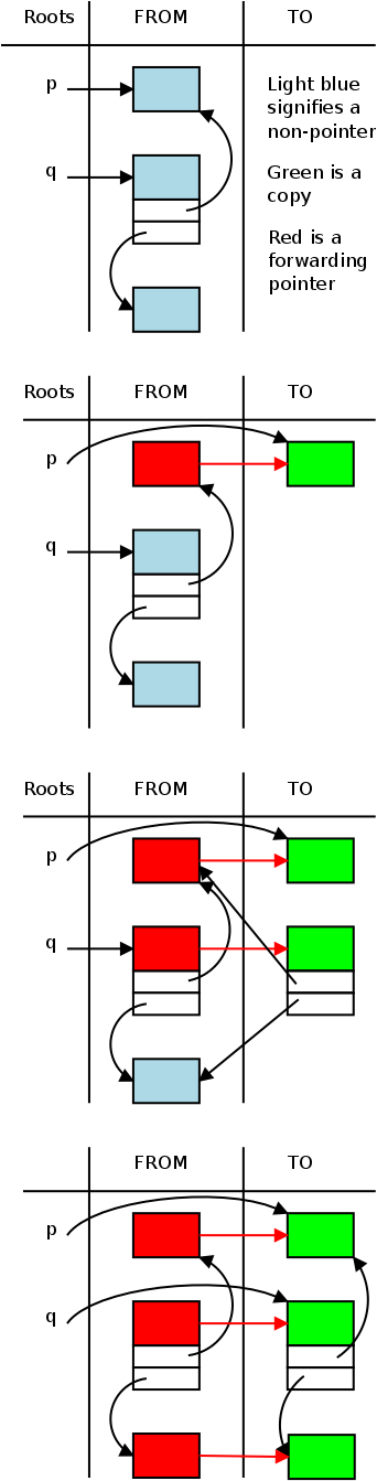
Divide the heap into two equal size pieces, often called
FROM
and TO
.
Initially, all allocations are performed using FROM; TO is unused.
When FROM is (nearly) full, garbage collection is performed.
During the collection, all the live data is moved from FROM to TO.
Naturally the pointers must now point to TO.
The tricky part is that live data may move while there are still
pointers to it.
For this reason a forwarding address
is left in FROM.
Once, all the data is moved, we flip the names FROM and TO and
resume program execution.
    Procedure GC is
       for each root pointer p
          p := traverse(p)
    Procedure traverse is
       if p.ALL is a forwarding address
          p := the forwarding address in p.ALL
          return p
       else
          newP := copy(p,TO)
          p.ALL := newP         -- write forwarding address
          for each pointers x in newP.ALL
             newP.x := traverse(newP.x)
          return newP
The movie on the right illustrates stop and copy in action.
- The top frame of the movie is the initial state.
There are two root pointers p and q, and three heap objects.
Initially p points to the first object, q points to the second.
The second object contains pointers to the other two.
- In the second frame we see the state after traverse has been
called with argument p and the assignment statement in GC has
been executed.
Note that traverse(p) executes the else arm of the if.
The object has been copied and the forwarding pointer set.
In this diagram I assumed that the forwarding pointer is the
same size as the original object.
It is required that an object is at least as large as a pointer.
The previous contents of the object have been overwritten by
this forwarding pointer, but no information is lost since the
copy (in TO space) contains the original data.
There are no internal pointers so the for loop is empty.
When traverse completes, p is set to point to the new object.
- The third frame shows the state while traverse(q) is in
progress.
The first two statements of the else branch have been executed.
The middle object has been copied and the forwarding pointer has
been set.
This forwarding pointer will never be used since there are no
other pointers to q.ALL.
Note that the two internal pointers refer to the old
(FROM-space) versions of the first and third objects.
Indeed, those pointers might have been overwritten by the
forwarding pointer, but again no information is lost since the
TO-space copy has the original values.
- The last frame shows the final state.
A great deal has happened since the previous frame.
The traverse(q) execution continues reaches the for loop.
This time there are two pointers in the copied block so traverse
will be called recursively two times.
The first pointer refers to an already-moved block so the then
branch is taken and, when traverse returns, the pointer is
updated.
The second pointer points to the original version of the third
block so the else branch is taken.
As in the top frame, the block is copied and the forwarding
pointer is set.
Again, when traverse returns, the pointer in the to-space copy
of the second block is updated.
Finally, traverse(q) returns and q is updated.
We are done.
The FROM space is superfluous, TO space is now what FROM space
was at the start.
Remarks
- Stop-and-copy compactifies with no additional code.
Specifically, the copies into TO space are contiguous so when
garbage collection ends, there is no external fragmentation.
- With mark-and-sweep, the garbage is moved, but the live
objects are not.
Thus, when collection ends, we have the in-use and free blocks
intersperses, i.e., external fragmentation.
Extra effort is needed to compactify.
- It has been observed that most garbage is
fresh, i.e., newly created.
Generational collectors separate out in-use blocks that
have survived collections into a separate region, which is
garbage collected less frequently.
- As described above, both mark-and-sweep and
stop-and-copy assume that no activity occurs during a pass of
the collector.
With multiprocessors (e.g., multicore CPUs) it is intriguing to
consider have the collector run simultaneous with the user
program (the so-called mu tater)
    procedure f is
       x : integer;
    begin
       x := 4;
       declare
          x : float;
       begin
          x := 21.75;
       end;
    end f;
Homework: CYU p. 121 (2, 4, 9)
Homework: Give a program in C that would not work
if local variables were statically.
3.3: Scope Rules
The region of program text where a binding is active is called the
scope of the binding.
Note that this can be different from the lifetime.
The lifetime of the outer x in the example on the right is all of
procedure f, but the scope of that x has a hole where the inner x
hides the binding.
We shall see below that in some languages, the hole can be filled.
Static vs Dynamic Scoping
  procedure main is
     x : integer := 1;
     procedure f is
     begin
        put(x);
     end f;
     procedure g is
        x : integer := 2;
     begin
        f;
     end g;
  begin
     g;
  end main;
Before we begin in earnest, I thought a short example might be
helpful.
What is printed when the procedure main on the right is run?
That looks pretty easy, main just calls g, g just calls f, and f
just prints (put is ada-speak for print) x.
So x is printed.
Sure, but which x?
There are, after all, two of them.
Is is ambiguous, i.e., erroneous?
Since this section about scope, we see that the question is which x
is in scope at the put(x) call?
Is it the one declared in main, inside of which f is defined, or is
the one inside g, which calls f, or is it both, or neither?
For some languages, the answer is the x declared in main and for
others it is the x declared in g.
The program is actually written in Ada, which is statically scoped
(a.k.a. lexically scoped) and thus gives the answer 1.
How about Scheme, a dialect of lisp?
    (define x 1)
    (define f (lambda () x))
    (define g (lambda () (let ((x 2)) (f))))
We get the same result: when g is evaluated, 1 is printed.
Scheme, like, ada, C, Java, C++, C#, ... is statically scoped.
Is every language statically scoped?
No, some dialects of Lisp are dynamically scoped, as is
Snobol, Tex, and APL.
In Perl the programmer gets to choose.
    (setq x 1)
    (defun f () x)
    (defun g () (let ((x 2)) (f)))
In particular, the last program on the right, which is written in
emacs lisp, gives 2 when g is evaluated.
The two Lisps are actually more similar that they might appear on
the right:
The emacs Lisp defun (which stands for "define function") is
essentially a combination of Scheme's define and lambda.
3.3.1: Static Scoping
In static scoping, the binding of a name can be determined by
reading the program text; it does not depend on the execution.
Thus it can be determined at compile time.
The simplest situation is the one in early versions of Basic: There
is only one scope, the whole program.
Recall, that early basic was intended for tiny programs.
I believe variable names were limited to two characters, a letter
optionally follow by a digit.
For large programs a more flexible approach is needed, as given in
the next section.
3.3.2: Nested Subroutines, i.e., Nested Scopes
The typical situation is that the relevant binding for a name is
the one that occurs in the smallest containing block and the scope
of the binding is that block.
So the rule for finding the relevant binding is to look in the
current block (I consider a procedure/function definition to be a
block).
If the name is found, that is the binding.
If the name is not found, look in the immediately enclosing scope
and repeat until the name is found.
If the name is not found at all, the program is erroneous.
What about built in names such as type names (Integer, etc),
standard functions (sin, cos, etc), or I/O routines (Print, etc)?
It is easiest to consider these as defined in an invisible scope
enclosing the entire program.
Given a binding B in scope S, the above rules can be summarized by
the following two statements.
- B is available in scopes nested inside S, unless B is
overridden, in which case it is hidden.
- B is not available in scopes enclosing S.
Some languages have facilities that enable the programmer to
reference bindings that would otherwise be hidden by statement 1
above.
For example
- In Ada a reference S.Y can be used to access the binding of Y
declared in scope S even if there is a lexically closer scope.
- In C++ S::Y can be used to access the binding of Y is class S.
Similarly ::Y can be used to refer to the binding of Y in the
global scope (outside all classes).
  procedure outer is         procedure outer is
     x : integer := 6;           x : integer := 6;
     procedure inner is          procedure inner is
     begin                          x : integer := 88;
        put(x);                  begin
     end inner;                     put(x,outer.x);
  begin                          end inner;
    inner;                   begin
  end outer;                     inner;
                               end outer2;
Access to Nonlocal Objects
Consider first two easy cases of nested scopes illustrated on the
right with procedures outer and inner.
How does the left execution of inner find the binding to x?
How does the right execution of inner find both bindings of x?
We need a link from the activation record of the inner to the
activation record of outer.
This is called the static link or the
access link.
But it is actually more difficult than that.
The static link must point to the most recent
invocation of the surrounding subroutine.
Of course the nesting can be deeper; but that just means
following a series of static links from one scope to the next
outer one.
Moreover, finding the most recent invocation of outer is not
trivial; for example, inner may have been called by a routine
nested inside inner.
For the details see a compilers book or
my course notes.
3.3.3: Declaration Order
There are several questions here.
- Must all declarations for a block precede all other
statements?
In Ada the answer is yes.
Indeed, the declarations are set off by the syntax.
        procedure <declarations> begin <statements> end;
        declare <declarations> begin <statements> end;
In C, C++, and java the answer is no.
The following is legal.
int z; z=4; int y;
- Can one declaration refer to a previous declaration in the
same block?
Yes for Ada, C, C++, Java.
int z=4; int y=z;
- Do declarations take affect where the block begins (i.e., they
apply to the entire block except for holes due to inner scopes)
or do they start only at the declaration itself?
int y; y=z; int z=4;
In Java, Ada, C, C++ they start at the declaration so the
example above is illegal.
In JavaScript and Modula3 they start at the beginning of the
block so the above is legal.
In Pascal the declaration starts at block beginning, but can't
be used before it is declared.
This has a weird effect:
In inner declaration hides an outer declaration but can't be
used in earlier statements of the inner.
Scheme
Scheme uses let, let* and letrec to introduce a nested scope.
The variables named are given initial values.
In the simple case where the initial values are manifest constants,
the three let's are the same.
(let ( (x 2)(y 3) ) body) ; eval body using new variables x=2 & y=3
We will study the three when we do scheme.
For now, I just add that for letrec the scope of each declaration is
the whole block (including the preceding declarations, so x and y
can depend on each other), for let* the scope starts at the
declaration (so y can depend on x, but not the reverse) and for let
the declarations start at the body (so neither y nor x can depend on
the other).
The above is somewhat oversimplified.
Homework: 5, 6(a).
Declarations and Definitions
Many languages (e.g., C, C++, Ada) require names to be declared
before they are used, which causes problems for recursive
definitions.
Consider a payroll program with employees and managers.
    procedure payroll is
      type Employee;
      type Manager is record
         Salary :    Float;
         Secretary : access Employee;   --  access is ada-speak for pointer
      end record;
      type Employee is record
         Salary : Float;
         Boss :   access Manager;
      end record;
    end payroll;
These languages introduce a distinction between a
declaration, which simply introduces the name
and indicates its scope, and a definition,
which fully describes the object to which the name is bound.
Nested Blocks
Essentially all the points made above about nested procedures
applies to nested blocks as well.
For example the code on the right, using nested blocks, exhibits the
same hole in the scope
as does the code on the left, using
nested procedures.
    procedure outer is      declare
      x : integer;            x : integer;
      procedure inner is    begin
        x : float:            -- start body of outer x is integer
      begin                   declare
        -- body of inner        x : float;
      end inner;              begin
    begin                       -- body of inner, x is float
      -- body of outer        end;
    end outer;                -- more of body of outer. x again integer
                            end;
Redeclaration
Some (mostly interpreted) languages permit a redeclaration
in which a new binding is created for a name already bound in the
scope.
Does this new binding start at the beginning of the scope or just
where the redeclaration is written?
    int f (int x) { return x+10; }
    int g (int x) { return f(x); }
    g(0)
    int f (int x) { return x+20; }
    g(5);
Consider the code on the right.
The evaluation of g(0) uses the first definition of f and returns
10.
Does the evaluation of g(5) use the first f, the one in effect when
g was defined, or does it use the second f, the one in effect when
g(5) was invoked.
The answer is: it depends.
For most languages supporting redeclaration, the second f is used;
but in ML it is the first.
In other words for most languages the redeclaration replaces the old
in all contexts; in ML it replaces the old only in later uses, not
previous ones.
This has some of the flavor of static vs. dynamic scoping.
3.3.4: Modules
Will be done later.
3.3.5: Module Types and Classes
Will be done later.
3.3.6: Dynamic Scoping
We covered dynamic scoping already.
3.4: Implementing Scope
3.5: The Meaning of Names within a Scope
3.6: The Binding of Referencing Environments
3.7: Macro Expansion
This section will be covered later.
3.8: Separate Compilation
Chapter 4: Semantic Analysis
Chapter 5: Target Machine Architecture
Start Lecture #3
Chapter 6: Control Flow
Remark: We will have a midterm.
It will be 1 hour, during recitation.
It will not be either next monday or the monday
after.
6.1: Expression Evaluation
Most languages use infix notation for built in operators.
Scheme is an exception (+ 2 (/ 9 x)).
    function "*" (A, B: Vector) return Float is
      Result: Float :=0.0;
    begin
      for I in A'Range loop
        Result := Result + A(I)*B(I);
      end loop;
      return Result;
    end "*";
Some languages permit the programmer to extend the infix operators.
An example from Ada is at right.
This example assumes Vector has already been declared as a
one-dimensional array of floats.
A'R gives the range of the legal subscripts, i.e. the bounds of the
array.
With loops like this it is not possible to access the array out of
bounds.
6.1.1: Precedence and Associativity
Most languages agree on associativity, but APL is strictly right to
left (no precedence, either).
Normal is for most binary operators to be left associative, but
exponentiation is right associative (also true in math).
Why?
Languages differ considerably in precedence (see figure 6.1 in 3e).
The safest rule is to use parentheses unless certain.
Homework: 1.
We noted in Section 6.1.1 that most binary arithmetic operators are
left-associative in most programming languages.
In Section 6.1.4, however, we also noted that most compilers are
free to evaluate the operands of a binary operator.
Are these statements contradictory?
Why or why not?
6.1.2: Assignments
Assignment statements are the dominant example of side effects,
where execution does more that compute values.
Side effects change the behavior of subsequent statements and
expressions.
References and Values
There is a distinction between the container for a value
(the memory location
) and the value itself.
Some values, e.g., 3+4, do not have corresponding containers and,
among other things, cannot appear on the left hand side of an
assignment.
Otherwise said 3+4
is a legal r-value, but not a legal
l-value.
Given an l-value, the corresponding r-value can be obtained by
dereferencing.
In most languages, this dereferencing is automatic.
Consider
a := a + 1;
the first a gives the l-value; the second the r-value.
Boxing
  begin
    a := if b < c then d else c;
    a := begin f(b); g(c) end;
    g(d);
    2+3
  end
Orthogonality
The goal of orthogonality of features is to permit the features in
any combination possible.
Algol 68 emphasized orthogonality.
Since it was an expression-oriented language, expressions could
appear almost anywhere.
There was no separate notion of statement.
An example appears on the right.
I have heard and read that this insistence on orthogonality lead to
significant implementation difficulties.
Combination Assignment Operators
I suspect you all know the C syntax
a += 4;
It is no doubt often convenient, but its major significance is that
in statements like
a[f(i)] += 4;
it guarantees that f(i) is evaluated only once.
The importance of this guarantee becomes apparent if f(i) has side
effects, e.g., if f(i) modifies i or prints.
Multiway Assignment (and Tuples)
Some languages, e.g., Perl and Python, permit tuples to be assigned
and returned by functions, giving rise to code such as
    a, b  :=  b, a    -- swapping w/o an explicit temporary
    x, y  :=  f(5);   -- this f takes one argument and returns two results
6.1.3: Initialization
Avoids the problem where an uninitialized variable has different
values in different runs causing non-reproducible results.
Some systems provide default initialization, for example C
initializes external variables to zero.
To initialize aggregates requires a way to specify aggregate
constants.
Dynamic Checks
An alternative to have the system check during execution if a
variable is uninitialized.
For IEEE floating point this is free, since there are invalid bit
patterns (NaN) that are checked by conforming hardware.
To do this in general needs special hardware or expensive software
checking.
Definite Assignment
Some languages, e.g., Java and C#, specify that the compiler must
be able to show that no variable is used before given a value.
If the compiler cannot confirm this, a warning/error message is
produced.
Constructors
Some languages, e.g., Java, C++, and C# permit the program to
provide constructors that automatically initialize dynamically
allocated variables.
6.1.4: Ordering within Expressions
Which addition is done first when you evaluate X+Y+Z?
This is not trivial: one order might overflow or give a less precise
result.
For expressions such as f(x)+g(x) the evaluation order matters if
the functions have side effects.
Applying Mathematical Identities
6.1.5: Short-Circuit Evaluation
Sometimes the value of the first operand determines the value of
the entire binary operation.
For example 0*x is 0 for any x; True or X
is True for any X.
Not evaluating the second operand in such cases is called a
short-circuit evaluation.
Note that this is not just a performance improvement; short-circuit
evaluation changes the meaning of some programs: Consider 0*f(x),
when f has side effects (e.g. modifying x or printing).
We treat this issue in 6.4.1 (short-circuited conditions) when
discussing control statements for selection.
Homework: CYU 7.
What is an l-value? An r-value?
CYU 11.
What are the advantages of updating a variable with an
assignment operator, rather than with a regular assignment
in which the variable appears on both the left- and right-hand
sides?
6.2: Structured and Unstructured Flow
Early languages, in particular, made heavy use of unstructured
control flow, especially goto's.
Much evidence was accumulated to show that the great reliance on
goto's both increased the bug density and decreased the readability
(these are not unrelated consequences) so today
structured alternatives dominate.
A famous article (actually a letter to the editor) by Dijkstra
entitled
Go To Statement Considered Harmful
put the case before the
computing public.
Common today are
- Selection
- if statement
- case statement
- Iteration
- while and repeat loops
- for loops
- iterators (looping over a collection)
- Other
- goto: Only when necessary.
- call/return: Accomplishes more than flow control
- exceptions
- continuations: normally in functional languages
6.2.1: Structured Alternatives to goto
Common uses of goto have been captured by newer control statements.
For example, Fortran had a DO loop (similar to C's for), but had no
way other that GOTO to exit the loop early.
C has a break statement for that purpose.
Homework: 24.
Rubin [Rub87] used the following example (rewritten here in C) to
argue in favor of a goto statement.
    int first_zero_row = -1     /* none */
    int i, j;
    for (i=0; i<n; i++) {
      for (j=0; j<n; j++) {
        if (A[i][j]) goto next;
      }
      first_zero_row = i;
      break;
    next:;
    }
The intent of the code is to find the first all-zero row, if any, of
an n×n matrix.
Do you find the example convincing?
Is there a good structured alternative in C?
In any language?
Multilevel Returns
Errors and Other Exceptions
  begin                              begin
    x := y/z;                          x := y/z;
    z := F(y,z); -- function call      z := F(y,z);
    z := G(y,z); -- array ref          z := G(y,z);
  end;                               exception   -- handlers
                                       when Constraint_Error =>
                                         -- do something
                                     end;
The Ada code on the right illustrates exception handling.
An Ada constraint error
signifies using an incorrect value,
e.g., dividing by zero, accessing an array out of bounds, assigning
a negative value to a variable declared positive
, etc.
Ada is statically scoped but constraints have a dynamic flavor.
If G raises a constraint error and does not have its own handler,
then the constraint error is propagated back to the caller of G, in
our case the anonymous block on the right.
Note that G is not lexically inside the block so the constraint
error is propagating via the call chain not scoping.
    (define f
      (lambda (c)
        (c)))
    (define g
      (lambda ()
        ;; beginning of g
        (call-with-current-continuation f)
        ;; more of g
        ))
6.2.2: Continuations
A continuation encapsulates the current context, including the
current location counter and bindings.
Scheme contains a function
(call-with-current-continuation f)
that invokes f, passing to it the current continuation c.
The simplest case occurs if a function g executes the invocation
above and then f immediately calls c.
The result is the same as if f returned to g.
This example is shown on the right.
However, the continuation is a object that can be further passed
on and can be saved and reused.
Hence one can get back to a given context multiple times.
Moreover, if f calls h giving it c and h calls c, we are back in g
without having passed through f.
One more subtlety: The binding that contained in c
is writable
.
That is, the binding is from name to memory-location-storing-the
name, not just from name to current-value.
So in the example above, if f changes the value of a name in the
binding, and then calls c, g will see the change.
Continuations are actually quite powerful and can be used to
implement quite a number of constructs, but the power comes with a
warning: It is easy to (mis-)use continuations to create extremely
obscure programs.
6.3: Sequencing
    for I in 1..N loop
      -- loop body
    end loop;
Many languages have a means of grouping several statements together
to form a compound statement
.
Pascal used begin-end pairs to form compound statements, C shortened
it to {}.
Ada doesn't need {} because the language syntax already contains
bracketing constructs.
As an example, the code on the right is the Ada version of a simple
C for loop.
Note that the end
is part of the for statement and not a
separate begin-end compound.
When declarations are combined with a sequence the result is a
block.
A block is written
{ declarations / statements } declare declarations begin statements end
in C and Ada respectively.
As usual C is more compact, Ada more readable.
Another alternative is make indentation significant.
I often use this is pseudo-code; B2/ABC/Python and Haskell use it
for real.
  if condition then statements
  if (condition) statement

  if condition then
    statements_1
  else
    statements_2
  end if

  if condition_1 {
    statements_1 }
  else if condition_2 {
    statements_2}
  else {
    statements_3}

  if condition_1 then
    statements_1
  elsif condition_2 then
    statements_2
  ...
  elsif condition_n then
    statements_n
  end if
6.4: Selection
Essentially every language has an if statement to use for selection.
The simplest case is shown in the first two lines on the right.
Something is needed to separate the condition from the statement.
In Pascal and Ada it is the then keyword;
in C/C++/Java it is the parentheses surrounding the condition.
The next step up is if-then-else, introduced in Algol 60.
We have already seen the infamous dangling else
problem that
can occur if statements_1 is an if.
If the language uses end markers like end if, the
problem disappears; Ada uses this approach, which is shown on the
right.
Another solution, used by Algol 60, is to forbid a
then to be followed immediately by
an if (you can follow then by a
begin block starting with if).
When there are more than 2 possibilities, it is common to employ
else if.
The C/C++/Java syntax is shown on the right.
This same idea could be used in languages featuring
end if, but the result would be a bunch
of end if statements at the end.
To avoid requiring this somewhat ugly code, languages like Ada
include an elsif which continues the
existing if rather than starting a new one.
Thus only one end if is required as we see in the
bottom right example.
6.4.1: Short-Circuit Conditions (and Evaluation)
Can if (y==0 || 1/y < 100)
ever divide by zero?
Not in C which requires short-circuit evaluation.
In addition to divide by zero cases, short-circuit evaluation is
helpful when searching a null-terminated list in C.
In that situation the idiom is
while (ptr && ptr->val != value)
The short circuit evaluation of && guarantees that we will
never execute null->val.
But sometimes we do not want to short-circuit the evaluation.
For example, consider f(x)&&g(x) where g(x) has a desirable
side effect that we want to employ even when f(x) is false.
In C this cannot be done directly.
  if C1 and C2  -- always eval C2
  if C1 and then C2 -- not always
Ada has both possibilities.
The operator or always evaluates both arguments;
whereas, the operator or else does a short circuit
evaluation.
Homework: 12.
Neither Algol 60 nore Algol 68 employs short-circuit evaluation for
Boolean expressions.
In both languages, however, an
if...then...else construct can be used as an expression.
Show how to use if...then...else to achieve the effect of
short-circuit evaluations.
  case nextChar is
    when 'I'    => Value := 1;
    when 'V'    => Value := 5;
    when 'X'    => Value := 10;
    when 'C'    => Value := 100;
    when 'D'    => Value := 500;
    when 'M'    => Value := 1000;
    when others => raise InvalidRomanNumeral;
  end case;
6.4.2 Case/Switch Statements
Most modern languages have a case or switch statement where the
selection is based on the value of a single expression.
The code on the right was written in Ada by a student of ancient
Rome.
The raise instruction causes an exception to be raised and thus
control is transferred to the
appropriate handler.
A case statement can always be simulated by a sequence of if
statements, but the case statement is clearer.
(Alternative) Implementations
In addition to increased clarity over multiple if statements, the
case statement can, in many situations be compiled into better code.
Most languages having this construct require that the tested for
values ('I', 'V', 'X', 'C', 'D', and 'M' above) must be computable
at compile time.
For example in Ada, they must be manifest constants, or ranges such
as 5..8 composed of manifest constants, or a disjunction of these
(e.g., 6 | 9..20 | 8).
In the simplest case where each choice is a constants, a jump
table can be constructed and just two jumps are executed,
independent of the number of cases.
The size of the jump table is the range of choices so would be
impractical if the case expression was an arbitrary integer.
If the when arms formed consecutive integers, the implementation
would jump to others if out of range (using comparison operators)
and then use a jump table for the when arms.
Hashing techniques are also used (see 3e).
In the general case the code produced is a bunch of tests and
tables.
Syntax and Label Semantics
The languages differ in details.
The words case
and when
in Ada become switch
and case
in C.
Ada requires that all possible values of the case expression be
accounted for (the others construct makes this
easy).
C and Fortran 90 simply do nothing when the expression does not
match any arm even though C does support a default
arm.
  switch (x+3) {
    case 2:  statements_2
             break;
    case 1:  statements_1
             break;
    case 6:  statements_6   // NO break between
    case 5:  statements_5   // cases 6 and 5
             break;
    default: something
  }
The C switch Statement
The C switch statement is rather peculiar.
There are no ranges allowed and the cases flow from one to the other
unless there is a break, a common cause of errors for beginners.
So if x is 3, x+3 is 6 and both statements_6 and statements_5 are
executed.
Indeed, the cases are really just statement labels.
This can lead to quite unstructured code including the infamous ...
Duff's Device (R Rated—Don't Show This to Minors)
  void send (int *to, int *from, int count) {
    int n = (count + 7) /8;
    switch (count % 8) {
      case 0: do { *to++ = *from++;
      case 7:      *to++ = *from++;
      case 6:      *to++ = *from++;
      case 5:      *to++ = *from++;
      case 4;      *to++ = *from++;
      case 3:      *to++ = *from++;
      case 2:      *to++ = *from++;
      case 1:      *to++ = *from++;
                 } while (--n > 0);
    }
  }
This function is actually perfectly legal C code.
It was discovered by Tom Duff, a very strong graphics programmer,
formerly at Bell Labs now at Pixar.
The normal way to copy n integers is to loop n times.
But that requires n tests and n jumps.
Duff unrolled
the loop 8 times meaning that he looped n/8
times with each body copying 8 integers.
Unrolling is a well known technique, nothing new yet.
But, if n is say 804, then after doing 100 iterations with 8 copies,
you need to do one extra iteration to copy the last 4.
The standard technique is to write two loops, one does n/8
iterations with 8 copies, the other does n%8 iterations with one
copy.
Duff's device uses only one loop.
Compiler technology has improved since Duff created the device and
Wikipedia says that when it was removed from part of the
X-window system, performance increased.
6.5: Iteration
  for I in A..N loop statements end loop;
  for (int i=A; i<n; i++) { statements }
6.5.1: Enumeration-Controlled Loops
On the right we see the basic for loop from Ada and C.
Code Generation For for Loops
Possibilities / Design Issues (Semantic Complications)
There is a tension between flexibility and clarity.
An Ada advocate would say that for loops are just for iterating
over a domain; there are other (e.g., while) loops
that should be used for other cases.
A C advocate finds the for(;;) construct an expressive and concise
way to implement important idioms.
This tension leads to different answers for several design
questions.
- Evaluation of loop bounds:
Many languages evaluate the bounds only once, before the
iterations start; however, C and successors evaluate the clauses
in the for statement each iteration.
- Scope and mutability of loop index:
Many languages have the index (I above) automatically declared
to be local to the loop.
In the example C loop, I explicitly declared the index to be
local.
One difference between the two examples is that in Ada the index
I is a constant, which prevents both accidental and deliberate
change of the index by the statements in the loop body.
- Non-unit Increments:
Many languages, including C, permit the increment to be an arbitrary
value.
Indeed, in C the increment clause
need not increment at
all.
In Ada the increment is implicit; the result is that the loop
travels through the entire range specified after
in.
- Reverse Order Iterations:
One possibility that Ada does
offer is to travel backwards through the range using
for i in reverse A..N loop statements end loop;
- Non-numeric domains:
        declare
          type Weekday is (Mon, Tues, Wed, Thurs, Fri);
          I : Integer -- **NOT** used in loop below
        begin
          for I in Weekday loop
            statements
          end loop;
        end
Many languages, including Ada, permit the range to be any
discrete set.
So an enumeration type is permitted as shown on the right, but a
range of Floats is not.
- Null Loops:
What happens if N < A?
Nearly all languages execute no iterations.
That is, the termination test is performed before the body
executes.
A famous exception is Fortran, which tests at the bottom of the
loop and hence always executes at least one iteration.
  for (expr1; expr2; expr3) statements;

  expr1;
  while (expr2); {
    statements;
  }
  expr3;
6.5.2: Combination Loops
The C for loop is actually quite close to the
while loops we discuss below since the three clause
within the for can be arbitrary expressions,
including assignments and other side-effects.
Indeed the for loop on the right is defined by C to have the same
semantics as the while loop below it unless the statements in the
body include a continue statement.
Loops combining both enumeration and logical control are also found
in Algol 60 and Common Lisp.
6.5.3: Iterators
We saw above an example of a loop with range an enum
Weekday=(Mon,Tues,Wed,Thurs,Fri).
More generally, some languages, e.g., Clu, Python, Ruby, C++,
Euclid, and C# permit the programmer to provide an iterator
with any container (an object of a discrete type).
    for (thing=first(); anyMore(); thing=next()); {
      statements
    };
The programmer then writes first
, next
, and
anyMore
operators that in succession yield all elements of
the container.
So the generalization of the C for loop becomes
something like the code on the right.
As an example imagine a binary tree considered as a container of
nodes.
One could write three different iterators: preorder, postorder, and
inorder.
Then, using the appropriate iterator in the loop shown above would
perform a preorder/postorder/inorder traversal of the tree.
True Iterators
Iterator Objects
Iterating with First-Class Functions
Iterating without Iterators
Generators in Icon
6.5.5: Logically Controlled Loops
Essentially all languages have while loops of the
general form
while condition loop statements end loop;
In while loops the condition is tested each iteration before the
statements are executed.
In particular, if the condition is initially false,
no iterations are executed.
In fact all loops can be expressed using this form, for suitable
conditions and statements.
This universality
proves useful when performing
invariant/assertion reasoning and proving programs consistent with
their specifications.
  repeat statements until condition;
  do { statements } while (condition);

  first := true;
  while (first or else condition) loop
    statements
    first := false;
  end loop;
Post-test Loops
Sometimes we want to perform the test at the bottom of the loop
(and thus execute the body at least once).
The first two lines on the right show how this is done in Pascal and
C respectively.
The difference between the two is that the repeat-until construct
terminates when the condition is true; whereas, the do-while
terminates when the condition is false.
The do-while is more popular.
One language that has neither is Ada so code like the bottom right
is needed to simulate do-while.
  Outer: while C1 loop
    statements_1a
    Mid: while C2 loop
      statements_2a
      exit outer when condition_fini;
      inner:while C3 loop
        statements_3
        exit when condition_2b;
        exit mid when condition_1b;
      end loop inner;
      statements_2b
    end loop mid;
    statements_1b
  end loop outer;
Midtest Loops
More generally, we might want to break out of a loop somewhere
in the middle
, that is, at an arbitrary point in the body.
Many languages offer this ability, in C/C++ it is the
break statement.
Even more generally, we might want to break out of a nested loop.
Indeed, if we are nested three deep, we might want to end the two
innermost loops and continue with the outer loop at the point where
the middle loop ends.
In C/C++ a goto is needed to break out of several
layers; Java extends the C/C++ break with labels to
support multi-level breaks; and Ada uses exit to
break out and a labeled exit (as shown on the right) for multi-level
breaks.
For example, if condition_fini evaluates true, the
entire loop nest is exited; if condition_2b evaluates
true, statements_2b is executed; and if condition_1b
evaluates true, statements_1b is executed.
6.6: Recursion
We will discuss recursion again when we study subprograms.
Here we just want to illustrate its relationship to iteration.
6.6.1: Iteration and Recursion
Although iteration is indicated by a keyword statement such as
while
, for
, or loop
, and recursion is indicated
by a procedure/function invocation, the concepts are more closely
related than the divergent syntax suggests.
Both iteration and recursion are used to enable a section to be
executed repeatedly.
  #include <stdio.h>
  int summation (int (*f)(int x), int low, int high) {
      int total = 0;
      int i;
      for (i = low; i <= high; i++) {
          total += (*f)(i);
      }
      return total;
  }
  int square(int x) {
      return x * x;
  }
  int main (int argc, char *argv[]) {
      printf ("Ans is %d", summation(&square,1,3));
      return 0;
  }

  (define square (lambda (x) (* x x)))
  (define summation
    (lambda (f lo hi)
      (cond
       ((> lo hi) 0)
       ((= lo hi) (f lo))
     (else (+ (summation f lo (- hi 1)) (f hi))))))
  (summation square 1 3)

  (summation (lambda (x) (* x x)) 1 3)
On the right we see three versions of a function to compute
Sum (from i = lo) (to i = hi) f(i)
given three parameters, lo, hi, and (a pointer to) f.
- The first version uses iteration.
It is written in C, which does not support passing functions as
parameters, but does support passing pointers to functions.
This explains the specification of the first parameter of
summation.
As an aside, C is willing to do some automatic type conversions
(called coercions) so the & could be omitted and the loop
body could say f(i).
However, it is important to note that the first argument to
summation is a pointer not a function.
- The second version is in scheme and uses recursion.
The reason the recursion goes down from hi rather than up from
lo is so that the arithmetic is done in the same order as with
the iterative version.
- The third version uses the same definition of summation as
does the second, but uses the anonymous function directly and
thus doesn't need (or have) any mention of the name square.
Tail Recursion
A recursive function is called tail recursive
if the last thing it does before returning is to
invoke itself recursively.
In this case we do not need to keep multiple
copies of the local variables since, when one invocation calls the
next, the first is finished with
its copy of the variables
and the second one can reuse them rather than pushing another set of
local variables on the stack.
This is very helpful for for performance.
  int gcd (int a, int b) {       int gcd (int a, int b) {
                               start:
    if (a == b) return a;          if (a == b) return a;
    if (a > b)                     if (a > b) {
        return gcd(a-b,b);              a = a-b; goto start; }
    return gcd(a,b-a); }           b = b-a; goto start; }
The two examples on the right are from the book and show equivalent
C programs for gcd: the left (tail-) recursive, the right iterative.
Both versions assume the parameters are positive.
Good compilers (especially, those for functional languages
will automatically convert tail recursive functions into equivalent
iterative form.
Thinking Recursively
I very much recommend the book The Little Schemer by
Friedman and Felleisen.
6.6.2: Applicative and Normal-Order Evaluation
Lazy Evaluation
6.7: Nondeterminacy
Start Lecture #4
Chapter 7: Data Types
Will be done later.
Chapter 8: Subroutines and Control Abstraction
Subroutines and functions are perhaps the most basic and important
abstraction mechanism.
They are found in all general purpose languages and many special
purpose ones as well.
Procedures vs. Functions: Applicative vs. Functional
Procedures are always applicative, they must be called for their side
effects since they do not return a value.
In a purely functional model (e.g., Haskell) functions are called
solely for their return value; they have no side effects.
These functions are like their mathematical namesakes:
they are simply a mapping from inputs to outputs.
Much more common is a hybrid model in which functions can have side
effects.
8.1: Review of Stack Layout
I do not cover this in detail here, since we cover it in some depth
in the
compilers class.
I just make a few points.

- As mentioned previously, stack-based storage is very efficient
and is used for data whose lifetime is that of the procedure in
which it is declared.
Since procedures have a LIFO-like behavior (last one called is
the first to return) a stack is an ideal storage model.
- Whenever a subroutine is called, it is given an activation
record (a.k.a. frame, or AR) on the stack.
- There are some subtleties to enable support for varargs in
languages like C.
These are mentioned later.
- There are normally two pointers into the stack.
- One points to the actual top of stack.
When a new AR is created it starts here.
The 3e calls this the stack pointer sp; the
dragon
book (a very common compiler text) calls it top.
(Technical point: The stack normally grows downward so the
top has the smallest address.)
- The other points into the middle.
The 3e calls it the frame pointer fp; the dragon book calls
it the top_sp.
The reason for the second pointer is that the objects of
unknown-at-compile-time size are all allocated at the top of
the AR.
Thus, the displacement from the value of sp to fixed size
objects is not known at compile time.
But the fp points below the varying size objects so its
displacement to each fixed size object is known at compile
time.
- Note that for each varying-size object we also store a pointer
to it.
These are of course a fixed size and hence are a fixed distance
from fp.
- Each AR has a pointer to the previous AR so that the stack can
be popped at subroutine return.
This is often called the dynamic link (3e)
or the control link (dragon).
Popping the stack is simply setting sp to the bottom of this AR
(a compile-time-constant distance below the current fp) and
setting fp to the dynamic link (stored a compile-time constant
distance from the current fp).
8.2: Calling Sequence
The caller and the callee cooperate to create a new AR when a
subroutine is called.
The exact protocol used is system dependent.
There are two parts to the calling sequence:
the prologue is executed at the time of the call,
the epilogue is executed at the time of the return.
Some authors use calling sequence just for the part done by the
caller and use prologue and epilogue just for the part done by the
callee.
I don't do this.
Saving and Restoring Registers
Some systems use caller-save; others use callee-save; still others
have some registers saved by the caller, other registers saved by
the callee.
Maintaining the Static Chain
In addition to the dynamic link, another inter-AR pointer is kept:
the static link (access link in dragon).
The static link points to the AR of the most recent activation of
the lexically enclosing block.
The static link is needed so that non-local objects can be
referenced (local objects are in the current AR).
It is not hard to calculate the static link during (the prologue
of) the calling sequence unless the language
supports passing subroutines as arguments.
We will not cover it; the simple case is again in the compiler
notes.
A Typical Calling Sequence
As mentioned previously, the exact details are system dependent,
what follows is a reasonable approximation.
The calling sequence begins with the caller:
- Pushes some registers on to the stack (modifying sp).
- Pushes arguments.
- Computes and pushes the static link.
- Executes a
call
machine instruction and pushes the
return address.
Next the callee:
- Pushes the old frame ptr and calculates the new one.
- Pushes some registers.
- Allocates space for temporaries and local variables.
- Begins execution of the subroutine.
When the subroutine completes, the callee:
- Stores the return value (perhaps on the stack).
- Restores some registers.
- Restores the sp.
- Restores the fp.
- Jumps to the return address, resuming the caller.
Finally, the caller:
- Restores some registers.
- Moves the return value to its destination.
Homework: CYU 5
Special Case Optimizations
8.2.1: Displays
8.2.2: Case Studies: C on the MIPS; Pascal on the x86
8.2.3: Register Windows
8.2.4: In-Line Expansion
8.3: Parameter Passing
Much of the preceding part of this chapter concerned compilers and
the implementation of programming languages.
When we study parameters, in particular parameter modes, we are
discussing the actual semantics of programs, i.e., what answers are
produced rather than how is it implemented.
However, many of the semantic decisions are heavily influenced by
implementation issues.
Most languages use a prefix notation for subroutine
invocation.
That is, the subroutine name comes first, followed by the arguments.
For applicative languages the arguments are normally parenthesized.
As we have seen in Lisp (e.g., Scheme) the function name is simply
the first member of list whose remaining elements are the arguments.
Another syntactic difference between most applicative languages and
Lisp is that, in the former, built in language constructs look quite
different from function application; whereas, in Lisp they look
quite similar.
Compare the following C and Scheme constructs for setting z to the
min of x and y.
    if (x < y) z = x; else z = y;
    (if (< x y) (set! z x) (set! z y))
    (set! z (if (< x y) x y))
Definitions:
Formal parameters
(often called simply parameters) are the names
that appear in the declaration of the subroutine.
Actual parameters
(often called simply arguments) refer to the
expressions passed to a subroutine at a particular call site.
8.3.1 Parameter Modes
The mode of a parameter determines the relation between the
actual and corresponding formal parameter.
For example, do changes to the latter affect the former.
There are a number of modes including.
- Call-by-value: The formal is bound to the
value of the actual.
The value of the actual is copied to the formal, but the
locations are distinct.
Hence changes to the formal do not affect the actual.
But see below for the effect when the formal and actual are
pointers.
- Call-by-reference: The formal is bound to the
location of the actual.
Most languages require the actual to be an l-value.
Changes to the former directly affect the latter.
- Call-by-value/result: The formal is bound to the
value of the actual.
When the routine returns, the actual is bound to the (final)
value of the formal.
These semantics appear to have the same effect as
call-by-reference, but see below.
Call-by-value/result is also referred to as call-by-copy-return.
- Call-by-name: The callee is macro-expanded
substituting the actuals for the formals (see below).
- Call-by-need: Similar to call-by-name (see below).
- Call-by-sharing: Essentially call-by-reference (not
discussed further).
  int c = 1;
  f(c);
  printf ("%d\n");
  ...
  void f(int x) { x = 5; }
Call-by-Value
When using call-by-value semantics, the argument is evaluated (it
might by an expression) and the value is assigned to the parameter.
Changes to the parameter do not affect the
argument, even when the argument is a variable.
This is the mode used by C.
Thus the C program on the right prints 1.
As most C programmers know, g(&x); can change the
value of x in the caller.
This does not contradict the above.
The value of &x can not be changed by g().
Naturally, the value of &x can be used by g().
Since that value points to x, g() can use &x to change x.
As most C programmers know, if A is an array, h(A) can
change the value of elements of A in the caller.
This does not contradict the above.
The extra knowledge needed is that in C writing an array without
subscripts (as in h(A) above) is defined to mean the
address of the first element.
That is, h(A) is simply shorthand
for
h(&A[0]).
Thus, the h(A) example is essentially the same as the
g(&x) example preceding it.
In Java, primitive types (e.g., int) are passed by value.
Although the parameter can be assigned to, the argument is not
affected.
Call-by-Reference
The location of the argument (the argument must be an l-value, but
see the Fortran exception below) is bound the parameter.
Thus changes to the parameter are reflected in the argument.
Were C a call-by-reference language (it is not)
then the example on the upper right would print 5.
By default pascal uses call-by-value, but if a parameter is
declared var, then call-by-reference is used.
Fortran is a little weird in this regard.
Parameters are normally call-by-reference.
However, if the argument is not an l-value, a new variable is
created, assigned the value of the argument, and is itself passed
a call-by-reference..
Since this new variable is not visible to the programmer, changes by
the callee to the corresponding parameter are not visible to the
program.
In Java, objects are passed by reference.
If the parameter is declared final it is readonly.
  with Ada.Integer_Text_IO; use Ada.Integer_Text_IO;
  procedure ScalarParam is
     A : Integer := 10;
     B : Integer;
     Procedure F (X : in out Integer; Ans : out Integer) is
     begin
        X := X + A;
        Ans := X * A;
     end F;
  begin
     F(A,B);
     Put (B);
  end ScalarParam;

  with Ada.Integer_Text_IO; use Ada.Integer_Text_IO;
  procedure Ttada is
     type IntArray is array (0..2) of Integer;
     A : IntArray := (10, 10, 10);
     B : Integer;
     Procedure F (X : in out IntArray; Ans : out Integer) is
     begin
        X(0) := X(0) + A(0);
        Ans  := X(0) * A(0);
     end F;
  begin
     F(A,B);
     Put (B);
  end Ttada;
Call-by-Value/Result
With call-by-value/result the value in the argument is copied into
the parameter during the call, and, at the return, the value in the
parameter (the result
) is copied back into the argument.
Certainly this copying is different from call-by-reference, but the
effect seems to be the same: changes to the parameter during the
subroutine's execution are reflected in the argument after the
return.
However, in the face of aliasing, call-by-value/result can differ
from call-by-reference as illustrated in the top Ada program on the
right.
Clearly the first assignment statement sets X to 20 which will,
eventually, be transmitted back to A.
The question is what value of A is used in the next assignment
statement: call-by-reference says the value is 20 (so 400 is
printed); whereas, call by value/result says the value is 10 (so 200
is printed).
In Ada, scalar arguments and parameters are call-by-value/result so
the answer printed is 200.
However, the program just below is basically the same, but uses
arrays.
In such cases the language permits either call-by-reference or
call-by-value/result.
The language reference manual warns users that programs, like this
one, whose result depends on the choice between call-by-reference
and call-by-value/result have undefined semantics.
The ada implementation on my laptop (gnat) uses call-by-reference
and therefore prints 400.
The Euclid language outlaws the creation of such aliases.
Call-by-Name
Call-by-name, made famous 40 years ago in Algol 60, will perhaps
seem a little weird when compared to the currently more common modes
above.
In fact it is quite normal today, just not for subroutine
invocation.
One should compare it to macro expansion, for example #define in the
C programming language.
One should remember that in 1960, the most widely used programming
languages were assembly languages and macro expansion was very
common.
If the parameter is not encountered while executing the subroutine,
the argument is not evaluated.
As in macro expansion, the argument is re-evaluated every time it
is used.
More significantly, it is evaluated in the context of the caller not
the callee.
This last point causes significant difficulty for the
implementation.
Remember that the caller and callee are compiled separately.
Thus the mechanism used is that the caller passes to the callee, not
only the argument, which can be an expression, but also the
referencing environment of the caller so that the expression can be
evaluated correctly every time it is used.
Traditionally, this referencing environment is called a
thunk.
As C programmers know, it is wise to have extra
parentheses; these were automatically supplied.
Also the names of local variables in the callee were automatically
made not to clash with the names of the parameters.
Call-by-Need
This can be view as a lazy
approximation of call by name.
The first time the parameter is encountered in the subroutine
execution, the value is calculated and saved.
This value is then reused if the parameter is encountered again.
Variations on Value and Reference Parameters
We discussed this above (call-by-value/result)
Call-by-Sharing
We do not discuss the subtle difference
between call-by-sharing and call-by-reference.
The Purpose of Call-by-Reference
There are two reasons to use call-by-reference instead of
call-by-value (assuming both are available).
- To enable the called routine to change the value of the
argument.
- To save copying a large argument to the corresponding parameter.
Be careful: it is often unwise to make semantic
choices for performance reasons.
Read-Only Parameters
Some languages permit parameters to be declared readonly
.
This means that the value of the parameter cannot be altered in the
callee, which naturally implies that the corresponding argument will
not have its value changed.
Modula-3 actually uses the word READONLY
;
C and C++ use const
.
Parameter Modes in Ada
An Ada programmer may declare each procedure parameter to have mode
in, out, or in out.
The default is in and all function parameters are required
to have mode in.
These modes do not describe the implementation (e.g., value
vs. reference), which we have discussed
above.
Instead they describe the flow of information between caller and
callee.
That is, they concern semantic intent, not implementation.
As the names suggest, an in parameter can be read by the
callee, but not written; whereas, an in out parameter can
be both read and written.
Both in and in out parameters initially have the
value of the corresponding argument.
In addition, the final value of an in out parameter,
becomes the value of the argument when the procedure returns.
Hence this argument must be an l-value.
An out parameter is similar to an in out
parameter.
The difference is that the initial value in the callee is
undefined.
  int f (int x);
  int g (int *x);
  int h (int &x);
References in C++
Like C, C++ is a call-by-value language—but with a twist.
Specific parameters can be declared to be call-by-reference simply
by preceding their names with an &.
Compare the three C++ function declarations on the right.
We have already seen examples like the first two before; they are
both legal in C.
The first one includes a standard call-by-value integer parameter x.
Changes to x in f are not visible to the caller.
The function g contains a call-by-value pointer
argument x (recall that int *x means that *x is an
integer, so x is a pointer to an integer).
The caller issues a statement such as g(&a), with
a declared as an integer, theryby passing
by value the pointer &a.
Function g cannot change &a, but can use it to modify
a.
Again, this is completely standard call-by-value semantics.
The declaration of h is a C++ extension to C.
Unlike the analogy to int *x (and
many other C declarations), int &x does
not mean that &x is an integer (that wouldn't
make sense, what would x be?).
Instead, it means that x is an integer that has been passed by
reference.
Similarly, the caller issues a statement such as h(a), with
a declared an integer.
To a beginner, it is, at the least, surprising that both &a and
*a, which in some ways have opposite semantics,
here both are used to indicate that a can be changed by the
caller.
  procedure main()
    procedure outer(i:int; procedure P)
      procedure inner
      begin
        print i
      end inner
    begin
      if i=1 then outer(2, inner)
      else P
    end outer
  begin main
    outer(1,main)
  end main
Closures as Parameters (Passing Nested Subroutines)
Consider the code on the right, using lexical (static) scoping.
Procedure outer has two parameters, the second of which
f is itself a procedure.
Procedure outer has a declaration of a nested procedure
inner.
The first time outer is invoked it calls itself passing
the procedure inner.
The second time outer is invoked, it calls its parameter
P which is bound to inner.
When inner is called it must be able to reference not only
its own declarations, but also the declarations in outer.
Since outer is called twice, we must arrange for the
correct outer environment to be visible to inner.
Since, in this example the inner that is called was
declared in the first invocation of
outer, the value 1 is printed.
Note that the outer that actually called inner
had i=2, but that is not relevant since we are assuming static
scoping.
Thus the first outer must pass to the second one the
referencing environment of inner (which, as we said,
includes the declarations in outer).
In other words, outer must pass to sub the
closure of inner.
To repeat, nested procedures used as parameters complicates the
picture considerably and necessitates the use of closures.
A parameter that is a (pointer to a) non-nested
procedure does not cause this problem.
The nesting is required.
Functions that take other functions as arguments (and/or return
functions as results are called higher-order functions.
Programming languages that support functions taking function
pointers as arguments (e.g. C) can emulate higher order functions.
Higher-order functions complicate the implementation, but we have
not studied this.
In particular, a parameter that is a (pointer to a)
non-nested procedure does not
cause the problem seen in the above example.
Nesting is required for this problem to occur.
Homework: CYU 13, 14, 17.
Homework: 4, 6, 12.
8.3.2: Call-by-Name
Done previously.
8.3.3: Special-Purpose Parameters
Conformant Arrays
Default (optional) Parameters
Ada and C++ permit parameters to be specified with default values
to be used if there is no corresponding argument.
    procedure f (x : integer; y : integer :=1) return integer;
    int f (int x, int y = 1);
Named Parameters
Ada permits the caller to refer to parameters by name (rather than
position).
Thus given the first declaration below, the two following invocations are
equivalent.
    Function F (I : Integer; J : Integer; K : Integer);
    F(1,2,3);
    F(1, K=>3, J=>2);
Variable Numbers of Arguments
This is the famous varargs facility in C and friends.
printf("X=%d, Y=%d, Z=%d, and W=%d\n", X,Y,Z,Z)
The number of subsequent arguments is determined by the first
argument.
The caller knows how many arguments there are, but the callee code
must be prepared for an arbitrary number.
The solution is to have the frame pointer fp point to a location a
fixed distance from the first argument.
Then the prologue code in the callee can find this argument,
determine the number of additional arguments, and proceed from
there.
8.3.4: Function Returns
8.3.A: Parameter Passing in Certain Languages
There is no new material here.
Instead, some previous material is reorganized by language rather
than by concept.
Parameter Passing in C
Parameters are passed by value; the argument cannot be changed by
the callee.
Call by reference can be simulated by using pointers.
Readonly parameters can be declared using const
Parameter Passing in C++
Default is call-by-value as in C.
Call by reference can be simulated with pointers as in C but can
also be explicitly stated using &
Readonly parameters can be declared using const
Parameter Passing in Java
Primitive types (e.g., int) are passed by value; objects by
reference.
A parameter of primitive type can be assigned to but the argument is
not affected.
A object parameter can be declared readonly via final.
Parameter Passing in Ada
Semantic intent is separated from implementation.
The specific modes available to the programmerin,
out, and in out determine the former, not the
latter.
- in: Information flows from caller to callee.
The parameter can only be read.
This mode may be implemented by value or reference (scalars are
by value).
- out: Information flows from the callee to the caller.
The parameter is read/write, but unitialized.
This mode may be implemented by value/result or reference
(scalars are by value/result).
- in out: Information flows both ways.
The parameter is read/write.
This mode may be implemented by value/result (scalars are
by value/result).
Functions (as opposed to procedures) can have only in
parameters.
8.4: Generic Subroutines and Modules
8.5: Exception Handling
8.6: Coroutines
8.7: Events
8.A: First-Class Functions
Another complication is first-class functions, that is
having the ability to construct functions dynamically and treat them
similarly to how other data types are treated.
One difficulty is that activation records are no longer stack like.
If procedure P builds function F dynamically and then returns it,
the activation record for P must be maintained since F may be called
later and needs the referencing environment of P where it was
created (assuming lexical scoping).
We shall see first-class functions in Scheme.
8.B: Recursion
As we have stated previously, it is the possibility of recursion
that forbids static allocation of activation records and forces a
stack-based mechanism.
Start Lecture #5
Remark: The room for the final exam has been moved
(by the department) from here 102 down the hall.
Chapter 9: Data Abstraction and Object Orientation
Done later.
Chapter 10: Functional Languages
10.1: Historical Origins
The pioneers in this work were mathematicians who were interested
in understanding what could be computed.
They introduced models of computation including the Turing Machine
(Alan Turing) and the lambda calculus (Alonzo Church).
We will not consider the Turing machine, but will speak some about
the lambda calculus from which functional languages draw
much inspiration.
10.2: Functional Progamming Concepts
Definition: The term
Functional Programming refers to a programming
style in which every procedure is a (mathematical) function.
That is, the procedure produces an output based on its inputs and
has no side effects.
The lack of side effects implies that no procedure can, for
example, read, print, modify its parameters, or modify external
variables.
By defining the stream from which one reads to be another input,
and the stream to which one writes to be another output, we can
allow I/O.
Some languages, such as Haskell are purely functional.
Scheme is not: it includes non functional constructs (such as
updating the value of a variable), but supports a functional style
where these constructs are used much less frequently than in a
typical applicative language.
Interesting Features found in Functional Languages
Having just described what is left out (or discouraged) in
functional languages, I note that such languages, including Scheme, have
powerful features not normally found in common imperative
languages.
- Functions are first-class values, meaning
that programs can create new functions at run-time, assign them
to variables, pass them as arguments, and return them from as
the value of a function.
The term first-class is to suggest that they have equal status
to other data types.
- With functions as first-class values, one can construct
higher-order functions, that is, functions
can accept functions as arguments and can return functions as
results.
- Since purely functional programming, does not permit
alteration of an existing object, aggregate objects must be
created all at once.
Hence functional languages permit functions to return
aggregates.
Homework: CYU 1, 4, 5.
Remark: We are moving the λ-calculus before
Scheme unlike the 3e.
10.6: Theoretical Foundatons
10.6.1: Lambda Calculus
Our treatment is rather different from the book.
The λ-calculus was invented by Alonzo Church in 1932.
It forms the underpinning of several functional languages such as
Scheme, other forms of Lisp, ML, and Haskell.
Technical point: There are typed and untyped variants of the lambda
calculus.
We will be studying the pure, untyped version.
In this version everything is a function
as we shall see.
Syntax
The syntax is very simple.
Parentheses are NOT use to show a function applied
to its arguments.
Let f be a function of one argument and let x be the argument we
want to apply f to.
This is written fx, no blank, no comma, no parens,
nothing.
Parentheses are used for grouping, as we show below.
Ignoring parens for a minute the grammar can be written.
    M → λx.M                a function definition
      | MN                  a function application
      | identifier          a variable, normally one character
The functions take only one variable, which appears before the dot;
the function body appears after the dot.
For example λx.x is the function that, given x, has value x.
This function is often called the identity.
Another example would be λx.xx.
This function takes the argument x and has value xx.
But what is xx?
It is an example of the second production in the above grammar.
The form xx means apply (the function) x to (the argument)
x.
Since essentially everything is a function, it is clear that
functions are first-class values and that functions are higher order.
Below are some examples shown both with and without parentheses
used for grouping.
    λx.x
    xxx                        (xx)x
    x(xx)
    λx.xx                      λx.(xx)
    (λx.x)x
    (λx.xx)(λx.xx)
    (λx.λy.yxx)((λx.x)(λy.z))
Examples on the same line are equivalent (i.e., the parens on the
right version are not needed).
The default without parens is that xyz means (xy)z, i.e., the
function x is applied to the argument y producing another function
that is applied to the argument z.
The variables need not be distinct, so xxx is possible.
The other default is that the body of a function definition extends
as far as possible.
Free and Bound Variables
Definitions:
- In a term λx.M, the scope of x is M.
- In a term λx.M, the variable x is called
bound in M.
- (Occurrences of) variables that are not bound are called
free.
- In a single term λx.M we can perform
α-conversion, that is, we can convert
the term to λw.M', where M' is M with all x's converted to w's.
β-Reduction
Since nearly everything is a function, it is expected that function
application (applying a function to its argument) will be an
important operation.
Definition: In the λ-calculus, function
application is called β-reduction.
If you have the function definition λx.M and you apply it to
N, (λx.M)N, the result is naturally M with the x's changed to
N.
More precisely, the result of β-reduction applied to
(λx.M)N is M with all free occurrences of x
replaced by N.
Technical point: Before applying the β-reduction above, we
must ensure (using α-conversions if needed) that N has no free
variables that are bound in M.
Do this example on the board: The β-reduction of
λx.(λy.yx)z is (λy.yz)=λy.yz
To understand the technical point consider the following
example λx.(λz.zx)z.
First note that this is really the same example as all I did to the
original is apply an α-transformation (y to z).
But if I blindly apply the rule for β-reduction to this new
example, I get (λz.zz)=λz.zz, which is clearly not
equivalent to the original answer.
The error is that in the new example M=(λz.zx),
N=z, and hence N does have a free variable that is bound in M.
Order of Evaluation
Consider the C-language expression f(g(3)).
Of course we must invoke g before we can
invoke f.
The reason is that C is call-by-value and we can't call f
until we know the value of the argument.
But in a call-by-name language like Algol-60, we call f
first and call g every time (perhaps no times) f
evaluates its parameter
Let's write this in the λ-calculus.
Instead of 3, we will use the argument λx.yx (remember
arguments can be functions) and for f and g we use the identity
function λx.x.
This gives (λx.x)((λx.x)(λx.yx)).
At this point we can apply one of two β-reductions,
corresponding to evaluating f or g.
Definition: The normal order
evaluation rule is to perform the (leftmost)
outermost β-reduction possible.
Definition: The
applicative order evaluation rule is to perform
the (leftmost) innermost β-reduction
possible.
Does the Order of Evaluation Matter
Doing one reduction using normal-order evaluation on our example
gives an answer of ((λx.x)(λx.xy)).
The outer (redundant) parentheses are removed and we get
(λx.x)(λx.xy).
If, instead, we do one applicative-order reduction we get the
same answer, but it seems for a completely different reason.
Must the answers always be the same?
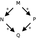
Do it again in class with the following more complicated example.
(λx.λy.yxx)((λx.x)(λy.z)).
In this case doing one normal-order reduction gives a different
answer from doing one applicative-order reduction.
But we have the following celebrated.
Church-Rosser Theorem: If a term M can be
β-reduced (in 0 or more steps) to two terms N and P, then there
is a term Q so that both N and P can be β-reduced to Q.
Corollary: If you start with a term M and keep
β-reducing it until it can no longer be reduced, you will
always get the same final term.
Definition: A term than cannot be β-reduced
is said to be in normal form.
Continue on the board to find the normal form of
(λx.λy.yxx)((λx.x)(λy.z)).
Does Every Term Have a Normal Form
That is, if you keep β-reducing, with the process terminate?
No.
Consider (λx.xx)(λx.xx).
Computability
Were this a theory course we would rigorously explain the notion of
computability.
In this class, we will be content to say that roughly speaking
computability theory studies the following question:
Given a model of computation, what functions can be computed?
There are many models of computation.
For example we could ask for all functions computable
- Using the untyped λ-calculus we just saw.
- Using the C programming language.
- Using the Ada programming language.
- Using a
Turing Machine
.
- Using many other models
A fundamental result is that for all the models listed the same
functions are computable.
Definition: Any model for which the computable
functions are the same as those for a Turing Machine is called
Turing Complete.
Thus, the fundamental result is that all the models listed above
are Turing Complete.
This should be surprising!
How can the silly λ-calculus compute all the functions
computable in Ada; after all the λ-calculus doesn't even have
numbers??
Or Boolean values?
Or loops?
Or Recursion?
I will just show a little about numbers.
Numbers in the λ-Calculus
First remember that the number three is a concept or an
abstraction.
Writing three as three
, or 3
, or III
,
or 0011
does not change the meaning of three.
What I will show is a representation of every non-negative number
and a function that corresponds to adding 1 (finding the successor).
Much more would be shown in a theory course.
It should not be surprising that each number will be represented as
a function taking one argument—that is all we have to work with!
The function with one parameter representing the number n
takes as argument a function f and returns function g taking one argument.
The function g will apply f n-times to its
argument.
I think those words are correct, but I also think the following
symbolism is clearer.
0 is represented as λf.λx.x
1 is represented as λf.λx.fx
2 is represented as λf.λx.f(fx)
3 is represented as λf.λx.f(f(fx)
So how do we represent the successor function S(n)=n+1?
It must take one argument n and produce a function that
takes an argument f and yields a function that applies f
one more time to its argument than n does.
Again the symbols may be clearer than the words
S is λn.λf.λx.f(nfx)
Show on the board that S1 is 2, i.e., show that
(λn.λf.λx.f(nfx))(λf.λx.fx)
is λf.λx.f(fx)
To make it clearer, first perform α-conversion to
λf.λx.fx and
get λg.λy.gy
Functions of More Than One Argument (Currying)
First note that in the expression λx.λy.z, the left
most function is higher order.
That is, it is given an argument x and it produces a function
λy.z.
Given (higher-order) functions of one variable, it is easy to
define functions of multiple variables by
λxy.z = λx.λy.z
This adds no power to the λ-calculus, but does make for
shorter notation.
For example, the successor function above is now written
S is λnfx.f(nfx).
10.6.2: Control Flow
This section shows how to model Boolean values, if-then-else, and
recursion.
Although I find it very pretty, I am skipping it.
10.6.3: Structures
This section shows how to model the Scheme constructs for list
processing, from which one can build many other structures.
Again, I am skipping it.
10.3: A review/Overview of Scheme
Lisp is one of the first high level languages, invented by John
McCarthy in 1958 while at MIT (McCarthy is mainly associated with
Stanford).
Many dialects have appeared.
Currently, two main dialects are prominent for standalone use:
Common Lisp and Scheme.
The Emacs editor is largely written in a Lisp dialect (elisp) and
elisp is used as a scripting language to extend/customize the
editor.
Whereas, Common Lisp is a large language, Scheme takes a more
minimalist approach and is design to have clear and simple
semantics.
Scheme was first described in 1975, so had the benefit of nearly 20
years of Lisp experience.
Notable Properties of Scheme
- Scheme uses call-by-value for
arguments/parameters.
- Scheme uses applicative-order evaluation, so
arguments are evaluated prior to function invocation.
This is expected for call-by-value.
EXCEPTION: Scheme has
special forms
that
have unique evaluation rules.
We shall discuss some later.
- Scheme is statically scoped
(a.k.a. lexically scoped).
Many Lisp dialects are either fully or partially dynamically
scoped.
- Scheme has a trivial syntax with
lots of parentheses.
- Scheme, like Lisp is homoiconic, i.e. the
primary representation of program code is the same structure that
is used for most data.
- Scheme is dynamically typed.
Values have types, but variables do not.
In particular, values of different types can appear in the same
variable (at different times of course).
Note, however, that Scheme encourages a functional style in which
variables do not change their value.
- Scheme has first-class functions.
Function creation commonly occurs during program execution;
functions can be arguments to other functions; and functions can
return other functions as results.
- Scheme implementations supply
garbage collection.
- Scheme supports continuations and
closures (explained later).
Interacting with Scheme
Scheme interpreters execute a read-eval-print loop.
That is, the interpreter reads an expression, evaluates the
expression, and prints the result, after which it waits to read
another expression.
It is common to use ⇒ to indicate the output produced.
Thus instead of writing
If the user types (+ 7 6), the interpreter replies 13
authors write
(+ 7 6) ⇒ 13
.
I follow this convention.
Note that the interpreter itself does not print ⇒; it simply
prints the answer 13
in the previous example.
Try ssh access.cims.nyu.edu; then ssh mauler; then mzscheme.
Illustrate the above in mzscheme.
There is a drscheme environment, you may wish to investigate.
Remark: Remember that you may implement labs on
any platform, but they must run at on the class platform, which is
mzscheme.
Scheme Syntax
The syntax is trivial; much simpler than other languages you know.
Every object in scheme is either an atom,
a (dotted) pair, or a list.
We will have little to say about pairs.
Indeed, some of the words to follow should be modified to take pairs
into consideration.
An atom is either a symbol (similar to an identifier in other
languages) or a literal.
Literals include numbers (we use mainly integers), Booleans
(#t and #f), characters (#\a, #\b, etc.; we won't use these much),
and strings ("hello", "12", "/usr/lib/scheme", etc.).
Symbols can contain some punctuation characters; we will manly use
easy symbols starting with a letter and containing letters, digits,
and dash (the minus sign).
For example, x23 and hello-world are symbols.
A list can be null (the empty list); or a list of elements, each of
which can be an atom or a list.
Some example lists:
    ()                       (a b c)
    (1 2 (3))                ( () )
    (xy 2 (x y ((xy)) 4))    ( () "")
    ( () () )                ( (()) (""))
Note that nested lists can be viewed as trees (the null list is
tricky).
Evaluating Expressions in Scheme
Evaluating Atoms in Scheme
Literals are self-evaluating, i.e., they evaluate to
themselves.
    453 ⇒ 453
    "hello, world" ⇒ "hello, world"
    #t ⇒ #t
    #\8 ⇒ #\8
Symbols evaluate to their current binding, i.e., they are
de-referenced as in languages like C.
This concludes atoms.
Evaluating Lists in Scheme
A list is a computation.
There are two types.
- Some lists are (special) forms, that is their first
element is a known keyword (e.g. define, lambda, etc.)
Each form comes with its evaluation rule.
- All other lists evaluate as follows.
- The first element is evaluated and must evaluate to an
operation.
- The remaining elements are evaluated.
- The operation is invoked, passing the values of the
remaining elements as arguments.
What if you want the list itself (or a symbol itself), e.g., what
if you want the data item ("hello" hello) and don't want to evaluate
"hello" on hello (indeed "hello" is not an operation so that would
be erroneous)?
Then you need a special form
, in this case the form
quote.
Some Standard (non-Special) Functions
We have already seen a few scheme functions
I remember define, lambda, + from lecture
one.
The third one + is not a special form.
The symbol + evaluates to a function and the remaining elements of
its list evaluate to the arguments.
The function + is invoked with these arguments and the result is
their sum.
Some Scheme Type-Predicate Functions
Since values are typed, but symbols are not, programs need a way to
determine the type of the value current bound to the symbol.
- (boolean? x) ; is x a boolean?
- (char? x) ; is x a character?
- (string? x) ; is x a string?
- (symbol? x) ; is x a symbol?
- (number? x) ; is x a number?
- (list? x) : is x a (proper) list?
- (pair? x) ; is x a (perhaps improper) list?
The book The Little Schemer
recommends
(define atom? (lambda (x) (and (not (pair? x)) (not (null? x)))))
I do this personally and sometime forget that atom? is not
part of standard Scheme.
Two other predicates are very useful as well
- (null? x) ; is x the null list?
- (zero? x) ; is x zero?
Some Scheme (Special) Forms
Compare
(+ x x) (lambda (x) (+ x x))
The second does not evaluate any of the x's.
Instead it does something special; in this case it creates an
unnamed function with one parameter x and establishes the body to be
(+ x x).
No addition is performed when the lambda is
executed (it is performed later when the created function is
invoked).
Quoting Data
Problem: Every list is a computation (or a special form).
How do we enter a list that is to be treated as data?
Answer: Clearly we need some kind of quoting mechanism.
Note that "(this is a data list)" produces a
string, which is not a list at all.
Hence the special form (quote data).
Quoting is used to obtain a literal symbol (instead of a variable
reference), a literal list (instead of a function call), or a
literal vector (we won't use vectors).
An apostrophe ' is a shorthand.
    (quote hello)                 ⇒ hello
    'hello                        ⇒ hello
    (quote (this is a data list)) ⇒ (this is a data list)
    '(this is a data list)        ⇒ (this is a data list)
10.3.1: Bindings
Scheme has four special forms for binding symbols to values:
define is used to give global definitions and the trio
let, let*, letrec are used for generating a nested scope
and defining bindings for that scope.
  (define x y)
  (define x "a string")
  (define f (lambda (x) (+ x x)))
On the right we see three uses of define.
The special
part about define is that it does
NOT evaluate its first parameter.
Instead, it binds that parameter to the value of the 2nd parameter,
which it does evaluate.
The form define cannot be used in a nested scope; One can
redefine an existing symbol so the first two functions on
the right can appear together as listed.
The third function is not any different from the first two: the
symbol f is bound in the global scope to the value computed
by the 2nd argument, which just happens to be a function.
All three let variations have the same general form
    (let                     ; or let* or letrec
      ( (var1 init1) (var2 init2) ... (var initn) )
      body    )              ; this ) matches (let
For all three variations, a nested environment is created, the
inits are evaluated, and the vars are bound in
to the values of the inits.
The difference is in the details, in particular, in the question of
which environment is used when.
For let, all the inits are evaluated in the
current environments, the new (nested) environment is formed by
adding bindings of the vars to the values of the
inits.
Hence none of the inits can use any of the vars.
More precisely, if an init mentions a var it
refers to the binding than symbol had in the current (pre-let)
environment.
For let*, the inits are evaluated and the
corresponding vars are bound in left to right order.
Each evaluation is performed in an environment in which the
preceding vars have been bound.
For example, init3 can use var1 and var2
to refer to the values init1 and init2.
For letrec a three step procedure is used
- All the vars are bound to uninitialized values.
- In this new environment, all the inits are
evaluated (in an unspecified order).
- Each var is then assigned the value of the
corresponding init.
  (letrec ((fact
            (lambda (n)
              (if (zero? n) 1
                 (* n (fact (- n 1)))))))
          (fact 5))
Thus any init that refers to any var is
referencing that var's binding in the new (nested) scope.
This is what is needed to define a recursive procedure (hence the
name letrec).
The factorial example on the right prints 120 and then exits the
nested scope so that typing (fact 5) immediately
after produces an error.
10.3.2: Lists and Numbers
There are three basic functions and one critical constant
associated with lists.
- (car l) ; returns the first element of the list l.
- (cdr l) ; returns the rest of l.
- (cons x l) ; prepends x onto l.
- () ; the null list (a constant).
In addition, some Schemers execute (define nil '()) so that
nil instead of '() can be used when the null list is desired.
  (car '(this "is" a list 3 of atoms)) ⇒ this
  (cdr '(this (has) (sublists))) ⇒ ((has) (sublists))
  (car '(x)) ⇒ x   (cdr '(x)) ⇒ '()
  (car '()) ⇒ error   (cdr '()) ⇒ error
List Decomposition: Car and Cdr
Another pair of names for car and cdr is, head and rest.
The car is the head of the list (the first element)
and the cdr is rest.
If we continue (for just a little while longer) to ignore pairs,
then we can say thatcar and
cdr are defined only for non-empty lists and that
cdr returns a (possibly empty) list.
List Decomposition Shortcuts: Cadr and Friends
Note that (car (cdr l)) gives the second element of a
list and hence is a commonly used idiom.
It can be abbreviated (cadr l).
In fact any combination of cxxxxr with each x (no more than
4 allowed) an a or d is defined.
For example, (cdadar l) is
(cdr (car (cdr (car l))))
  (cons 5 '(5)) ⇒ (5 5)   (cons 5 '()) ⇒ (5)
  (cons '() '()) ⇒ (())   (cons 'x '(()) ⇒ (x ())
  (cons "these" '("are" "strings")) ⇒ ("these" "are" "strings")
  (cons 'a1 (cons 'a2 (cons 'a3 '()))) ⇒ (a1 a2 a3)
List Building: Cons
The function (cons x l) prepends x onto the list
l.
It may seem that to get a list with 5 elements we need
5 cons applications, but there is a shortcut.
The function list takes any number of arguments (including
0) and returns a list of n elements.
It is equivalent to n cons applications the rightmost
having '() as the 2nd argument.
For example
(list 'a1 'a2 'a3) is equivalent to
(cons 'a1 (cons 'a2 (cons 'a3 '()))), the last example on
the right.
(Dotted) Pairs, Improper Lists, and Box Diagrams
You could very easily ask where the silly names car and cdr came
from.
Head or first make more sense for car, and rest makes more sense for
cdr.
In this section I briefly cover the historical reason for the
car/cdr terminology, hint at how lists are implemented, introduce
(dotted) pairs, show how our (proper) lists as well as improper
lists can be built from these pairs and present box diagrams, which
are another (this time pictorial) representation of lists, pairs,
and improper lists.
Lisp was first implemented on the IBM 704 computer that had 32,768
36-bit words.
Since 32,768 is 215, 15-bits were needed to address the
words.
A common instruction format (all instructions were 36-bits) had
15-bit address and decrement fields.
There also were address and decrement registers.
Typically, the pointer to the head of a list was the Contents of the
Address Register (CAR) and the pointer to the rest was the Contents
of the Decrement Register.
The car and cdr were stored in the address and decrement fields of
memory words as well.
Thus we see that the fundamental unit is a pair of pointers in
lisp.
This is precisely what cons always returns.
Box diagrams are useful for seeing
pictorially what a list looks like in terms of cons cells.
The referenced page is from the manual for emacs lisp, which has
some minor differences from scheme.
I believe the diagram is completely clear if you remember than nil
is often used for the empty list ('() in Scheme).
Each box-pair or domino depicts a cons cell and is written in
Scheme as a dotted pair (each box is one component of the pair).
Note how every list (including sublists) ends with a reference to
nil in the right hand component of the rightmost domino.
This corresponds to the fact that if you keep taking cdr (cddr,
cdddr, etc) of any list you will get to '() and then cdr is invalid.
This is the defining characteristic of a proper
list (normally called simply a list).
In fact the second argument to cons need not be a list.
The single domino improper
list beginning
this writeup on dotted pairs
shows the result of executing
(cons 'rose 'violet).
In this example the second argument is an atom, not a list.
The resulting cons cell can again be written as a dotted pair, in
this case it is (rose . violet).
Likewise, cdr is generalized to take this domino as input.
As before it returns the right hand box of the domino, in this
case violet.
Thus we maintain the fundamental identities
(car (cons a b)) is a and
(cdr (cons a b)) is b
for any objects a and b.
Previously b had to be a list.
The summary is that cons in generalized to not require a list for
the second argument, the resulting object is represented as a dotted
pair in scheme, and linking together dotted pairs gives a
generalized
list.
If the last dotted pair in every chain has cdr equal to '(), then
the generalized list is an ordinary list; otherwise it is
improper
.
(define (make-counter)
  (let ((count 0))
    (lambda () (set! count (+ 1 count))
               count)))
(define ctr1 (make-counter))
(define ctr2 (make-counter))
(ctr1)
(ctr2)
(ctr2)
(ctr2)
(ctr1)
Closures (not covered 2009-10 Fall)
Consider the code on the right.
When the first (define is executed, a new function
make-counter is created.
This is nothing new.
However, bundled with the function is the variable count.
Technically, count is part of the environment in which the
function is defined and the (define captures the entire
closure (i.e., the environment is included).
When the second and third (define's are executed, two
counters are created, each of which is initialized to zero and will
grow each time they are invoked.
thus the 5 function invocations that follow will print
1,2,3,4,2.
Homework: CYU: 9.
Homework: 1, 3.
Start Lecture #6
Remark: Review the meaning of free in M
.
Remark: Lab 2 was assigned last thursday it is
due 22 October 2009.
Remark: The midterm will be during recitation #8,
26 Oct.
A practice final is available.
Numbers in Scheme
Scheme has a wide variety of numbers, including rational number
(i.e., fractions).
Most implementations include arbitrary precision rationals.
We will stick to simple integers.
Vectors in Scheme
A vector is similar to an array but the elements may be of
heterogeneous type, similar to a record in Ada or a struct in C.
We will not study vectors.
10.3.3: Equality Testing and Searching
Boolean Values
Scheme has two Boolean constants, #t and #f.
However, when performing a test (e.g., in a control flow structure)
any value not #f is treated as true.
Eq?, Eqv? and Equal?
Scheme has three general comparison operators, the first two of
which are similar.
We will use only eq? and equal?.
  (eq 'a 'a)
  (let ((x 3) (y 3)) (eq? x y))
  (let ((x '()) (y '())) (eq? x y))
  (eq? 'x 'y) ⇒ #f
  (eq? (cons 2 3) (cons 2 3)) ⇒ #f
  (eq? "" "")  (eq "xy" "xy")
  (eq? 2 2)
  (eq? '(2 . 3) '(2 . 3))  ⇒ #t
  (eq? (list 2 3) (list 2 3)) ⇒ #f
  (equal? (lambda (x) x) (lambda (x) x))
The first eq? is cheap, it essentially just checks the
memory address.
So (eq 'a 'a) ⇒ #t because Scheme only keeps one symbol
a.
(If two locations had the symbol a, how could
a be evaluated?).
Similarly, Scheme keeps only one constant 3 so the second example on
the right yields #t.
There is also only one empty list so the next example also gives
#t.
Naturally the two symbols x and y are stored
separately, explaining the next example.
Each cons invocation produces a new cons cell (a new dotted
pair), explaining the next examples.
Implementations are given freedom on how to store strings so there
might be two copies of the same string.
Hence the next two examples (on one line) have undefined results.
They will, however, be either #t or #f.
The same is true for numbers (next example, eqv? would give #t).
Even though the dotted pair example that is next looks just like the
cons example, this time the result is unspecified.
The principle here is that the implementation is free to store all
uses of the same literals in the same location.
The next example is not a literal, but a cons (actually 2 cons) so
the result is #f.
The story for equal? is simpler.
A good rule of thumb is that if the two arguments print the
same, equal? evaluates to #t; otherwise #f.
The only unspecified case is for functions is the last example (both
mxscheme and scheme48 give #f)
We will show searching below, after introducing cond.
  (cond
     (pred1 expr1)
     (pred2 expr2)
     ...
     (predn exprn)
     (else def-expr)
  )
10.3.4: Control Flow and Assignment
Control Flow: Cond and If
Scheme actually has a number of special forms for control flow.
However, you can get by with just one, cond, a
case/switch-like construct, which is shown on the right.
It is a special form since not all arguments to cond are necessarily
evaluated and those that are evaluated have a special rule.
First pred1 is evaluated, if the value is not #f, it is considered
true and expr1 is evaluated.
This completes the evaluation of the cond; the value of the cond is
the value of expr1.
If pred1 evaluates to #f, the same procedure is applied to pred2,
etc.
If all n predi's evaluate to #f, def-expr is evaluated and that
becomes the value of the cond.
For simple tests if is convenient
(if (condition) (exprt) (exprf))
Again we have a special form.
First condition is evaluated.
If the value is #t, exprt is evaluated and that becomes the
value of the if.
If condition evaluates to #f, then exprf is
evaluated and that becomes the value of the if.
Control Flow: Sequencing and Do Loops
  (begin
    (expr1)
    ...
    (exprn)
  )
What do you do when the then
part of your code if is more
than one expression?
Or if this happens to one of the expri's in a
cont?
You need a grouping similar to {} in C.
You could use one of the let's, but that is overkill when
you don't need a new scope.
Instead you use the begin special form shown on the right.
The expri's in the begin form are all executed in order and
the value of the last one is the value of the begin.
The basic mechanism for iteration is recursion, but various looping
constructs are also available
I guess the keyword do was chosen for the looping form
because lisp was invented around the time of Fortran, but I do not
know.
You can always use recursion instead of a do loop; but the
do loop is in the book if you want to use it.
Assignment: The Bangs
The special forms involving assignment end in !, which is
pronounced bang (at least set! is pronounced set-bang; I am
not so sure about set-car! and set-cdr!.
The (side-) effect of set! is to change the value of its
first argument to the value of its second argument.
Again we have a special-form since the first argument is not
evaluated.
It is an error to set bang an undefined identifier; for that you
should use define or one of the let's.
The special functions set-car! and set-cdr!
change the car (resp. cdr) fields of their first argument to the
value of the second argument.
I advise against their use, as the results can be surprising.
For some reason, they don't appear to be available in mzscheme.
There are in scheme48 and also definitely appear in the scheme
manual so I am surprised.
But their absence is no great loss for us.
Ang found the missing mzscheme bangs.
They are part of a group of mutable
functions including mcons
that makes a cons cell you can mutate with the mutable bangs.
Recursion on Lists
Lists are the basic Scheme data structure and recursion is the
basic iteration construct so it is important to see how to use
recursion to step through the elements of a loop.
  (define member
    (lambda (elem lat)
      (cond
        ((null? lat) #f)
        ((eq? elem (car lat)) lat)
        (else (member elem (cdr lat))))))

(define count-members
  (lambda (a lat) (member1 a lat 0)))
(define member1
  (lambda (a lat count)
    (cond
     ((null? lat) count)
     ((eq? a (car lat))
      (member1 a (cdr lat) (+ 1 count)))
     (else (member1 a (cdr lat) count)))))
As an example the code on the right implements member, a
function with two parameters: elem an element
and lat a list of atoms (i.e., lat is a list and each
element is an atom, no sublists).
If the element does not appear in the list, member returns
#f.
It it does appear, member returns the suffix of the list
starting with the first occurrence.
We could return #t, but the above is more common.
Recall that everything except #f is viewed as true when testing, so
returning either the suffix or #t has the same effect when just
testing.
Sometimes it is helpful to have the rest of the list in hand,
perhaps for further searching.
The code sequence shown is fundamental for list operations, be
sure you understand it completely.
The second example counts the number of times a occurs in lat
This version of the program uses eq? for the testing.
We might want instead to use equal? or even
eqv?.
Thus we could write three versions of member and count-members just
changing
eq? to equal? and then to eqv?.
A better alternative is to use higher-order functions, as shown
below.
(define count-members-sexp
  (lambda (a s) (member2 a s 0)))
(define member2
  (lambda (a s count)
    (cond
     ((null? s) count)
     ((atom? (car s))
      (cond
       ((eq? a (car s))
        (member2 a (cdr s) (+ 1 count)))
       (else (member2 a (cdr s) count))))
     (else ;; the car is a sublist
      (+ (member2 a (car s) 0)
         (member2 a (cdr s) count))))))
Nested Lists and S-Expressions
An element of a list can itself be a list, for example
(1 (2 3)).
More generally a parenthesized sequence of symbols, with balanced
parenthesis is called an s-expression.
How do we write a program that can deal with a list containing
sublists?
The code on the right does this, again counting occurrences.
It assumes the sexp is a list possibly with sub-lists.
But it doesn't handle the case where the sexp is just an atom.
Homework: First, enhance the last example to
handle atoms as well.
Second, change the example code and your enhancement to use
if instead of cond where a simple if-then-else is
appropriate.
10.3.5: Programs as Lists
As mentioned previously, Scheme (and Lips in general) is homiconic,
or self-representing.
A parenthesized sequence of symbols, with balanced parenthesis is
called an s-expression whether the sequence represents a
list or a program.
Indeed, an unevaluated program is exactly a list.
We have seen that Scheme has a special form quote that
prevents evaluation.
In addition there is a function eval that forces
evaluation.
  (define fact-iter
    (lambda (prod lo hi)
      (if (> lo hi)
          prod
          (fact-iter (* prod lo)
                     (+ lo 1)
                     hi))))
  (define fact-tail (lambda (n) (fact-iter 1 1 n)))
10.3.A: Tail-Recursion Revisited
We have already noted that if the last action
performed by a function is a recursive call of itself (and there are
no other direct or indirect recursive calls of this function), then
a new AR is not needed and the recursion can be transformed into
iteration by a compiler.
The only new point to be made here is that sometimes a clever
programmer can turn a seemingly fully
recursive program into
a tail-recursive one, often by defining an auxiliary (a.k.a. helper)
function.
We begin with the fact procedure fact shown above when
discussing letrec above.
That fact executes a multiply after
evaluating its recursive call and thus is nottail
recursive; however the transformed version on the right is.
Homework: CYU 10.
Homework: 6, 8.
10.3.6: Extended Example: DFA Simulation
10.4: Evaluation Order Revisited
10.4.1: Strictness and Lazy Evaluation
10.4.2: I/O Streams and Monads
10.5: Higher-Order Functions (i.e., Functions as Arguments and Return Values)
Assume you need three functions for a physics research project.
All of them take as input the state of a system.
The first function returns the heaviest object,
The second function returns the densest object,
The third function returns the object having the highest kinetic
energy.
You could write three separate programs, but you notice that they
are all the same: they are determining a max but have different
definitions of less than.
Hmmm.
  (define make-member
    (lambda (test?)
      (lambda (elem lis)
        (cond
          ((null? lis) #f)
          ((test? elem (car lis)) lis)
          (else (member elem (cdr lis)))))))

  (define member-eq    (make-member eq?))
  (define member-eqv   (make-member eqv?))
  (define member-equal (make-member equal?))
Returning to the member example above, we want variants with
different comparison functions.
So let's pass in the desired comparison function and use that.
In more detail, write make-member as a function with one input, the
comparison function.
Make-member returns as result a function equivalent to member above
but using the given comparison function instead of having
eq? hard-wired in.
The result is shown on the right.
Again, this is a fundamental use of first-class functions, be
sure you understand it.
10.7: Functional Programming in Perspective
There is some evidence that functional programs are less buggy.
There is even greater evidence that applicative programming
dominates in the real world.
The question is why.
Current believe is that the reason is social not technical: more
courses, textbooks, libraries, etc.
Chapter 7: Data Types
We can think of a type as a set of values (the members of the
type).
A different question is how should the type be represented on the
computer (Intel Floating Point, IBM Floating Point, vs. IEEE Floating
Point; two's complement vs. one's complement for negative integers;
binary vs. hexadecimal vs. octal).
We will not discuss this second question.
Types can give implicit meaning to operations.
For example in Java + means concatenation if the operands are
strings and means addition if the operands are integers.
Type clashes, using a type where it is not permitted, often
indicates a bug and, if checked automatically by the run-time system
or (better, yet) by the compiler, can be a big aid in debugging.
7.1: Type Systems
A type system consists of:
- A mechanism ofr defining types and associating them with
language constructs
- A set of rules for
- Type equivalence: When do two objects
have the same type?
- Type compatibility: Where can
objects of a given type be used?
- Type synthesis/inference: How do you
determine the type of an expression from its parts or, in
some cases, from its context (i.e., the type of the whole is
used to determine the type of the parts).
The synthesis/inference terminology is not standardized.
Some texts, e.g., 3e, use type inference both for determining the
type of the whole from the type of its parts, and for determining the
type of the parts from the type of the whole.
Other texts, e.g., the Dragon book, use type synthesis for the
former and type inference for the latter.
Some languages are untyped (e.g., B the predecessor of C); we will
have little to say about those beyond saying that B actually had one
datatype, the computer word.
Types must be assigned to those constructs that can have values or
that can refer to objects that have values.
These include.
- Literal constants (e.g., 5.8, "hello").
- Named constants (e.g. static final int x = 3).
- Variables.
- Subroutines (not always, but having signatures is nice)
- More complicated expressions made up of these.
7.1.1: Type Checking
Definition: Type checking is
the process of ensuring that a program obeys the type system's type
compatibility rules.
Definition: A violation of the type checking rules
is called type clash.
Definition: A language is called
strongly typed if it prevents operations on
inappropriate types.
Definition: A strongly typed language is called
statically typed if the necessary checks can be
performed at compile time.
Note that static typing is a property of the language not the
compiler: A statically typed language could have a poor compiler
that does not perform all the necessary checks.
int main (void) {
    int *x;
    int y;
    int *z;
    z = x + y;
    return 0;
}

(define test
  (lambda ()
    (let ((x 5) (y '(4)))
      (+ x y))))

procedure Ttada is
   X : Integer := 1;
   type T is access Integer;
   Y : T;
begin
   X := X + Y;
end Ttada;
Strong vs Weak Typing
The key attribute of strongly typed languages is that variables,
constants, etc can be used only in manners consistent with their
types.
In contrast weakly typed languages offer many ways to bypass the
type system.
A good comparison would be original C vs (Ada or Scheme).
C has unions, varargs, and a deliberate confusion between pointers
and arrays.
Original C permitted many other type mismatches.
A motto for C is "Trust the programmer!".
Both Ada and Scheme are much tighter in this regard: both are
strongly typed, Ada is (mostly) statically typed.
Compare the three programs on the right.
The C program compiles and runs without errors!
The Scheme define is accepted, but (test) gives
an error report.
The Ada program doesn't even compile.
Static vs Dynamic (Strong) Type Systems
Static and Dynamic strongly typed systems both prevent type
clashes, but the prevention is done at different times and by
different methods.
In a static type system
- Variables and values are typed.
- The compiler (interpreter) enforces type rules at
compile (definition) time.
In a dynamic type system
- Variables are not typed; values are typed.
- The compiler (interpreter) enforces type rules at
run time.
Ada, Pascal, and ML have static type
systems.
Scheme (Lisp), Smalltalk, and scripting languages
(if strongly typed) have dynamic type systems.
These systems typically have late binding as well.
A mixture is possible as well.
Ada has a very few run-time checks; Java a few more.
Static type systems have the following advantages.
- Faster execution: The run-time checks are avoided.
- Typically, better (more extensive) error checking, with errors
reported sooner.
- The resulting program is easier to read and maintain.
Dynamic type systems have the following advantages.
- They are more flexible.
- Programs are easier to write.
7.1.2: Polymorphism
Definition: Polymorphism
enables a single piece of code to work with objects of multiple
types.
Definition: In
parametric polymorphism the type acts as though
it is an extra unspecified parameter to every operation.
Consider dynamic typing as use in Scheme.
Depending on the type of the operands, the addition operator + can
indicate, integer arithmetic, real arithmetic, or
infinite precision
arithmetic.
If the operands are of inappropriate type, + signals an error.
Since the type was never specified by the programmer, this is often
called implicit parametric polymorphism.
fun len xs =
  if null xs
  then 0
  else 1 + len (tl xs)
The example on the right is written ML, which is statically typed,
yet still manages to support implicit parametric polymorphism.
The (very slick) idea is that ML supports type inference so is able
to deduce individual types from the type of an expression.
In this case the interpreter determines that the type of the len
function as 'a list→int, i.e., a function with
parameter a list of type 'a (unknown) and result integer.
Consider instead generics in Ada and Java and
templates in C++.
In this case the programmer writes code for each type and system
chooses which one to invoke depending on the type.
This is called explicit parametric polymorphism.
We will soon learn that the positive integers can be considered a
subtype of the integers and that a value in a subtype can be
considered a value on the supertype.
This is called subtype polymorphism.
Similarly, the ability to consider a class as one of its
superclasses is called class polymorphism.
7.1.3: The Meaning of Type
Types can be though of in at least three ways, which we will
briefly describe.
They are the denotational
, constructive
, and
abstraction-based
viewpoints.
With denotational semantics:
- A type is simply a set T of values.
- A value has type T if it belongs to the set.
- An object has type T if it is guaranteed to be bound
to a value in T.
An advantage of denotational semantics is that composite types,
e.g., arrays and records, can be described using standard
mathematical operations on sets.
With constructive semantics:
- A type is either built-in or
- Constructed from basic-in or other
constructed type using a type-constructor
(record, array, etc).
With abstraction-based semantics, a type is an
interface consisting of a set of operations with
well defined, consistent semantics.
It is characteristic of object-oriented languages.
In practice, we normally think of a type using all three
viewpoints.
7.1.4: Classification of Types
We will first discuss several scalar types and
then composite types that consist of aggregates of
both scalar and other composite types.
Scalar Types
Discrete Types
The term discrete comes from mathematics, where it is contrasted
with continuous.
A type is considered discrete if there is a clear notation of
successor and predecessor for values in the type.
Mathematically, this gives is an isomorphism between the elements of
the type and a consecutive subset of integers.
Indeed, the basic examples of discrete types are the integers
themselves and enumeration types.
Integers.
Of course with only a finite number of bits to use for the
representation (most commonly 16, 32, or 64), the
integer type
is really just a finite subset of the
mathematical integers.
- Some languages (e.g. C/C++, C#, Ada) have both signed and
unsigned variants.
- Ada has predefined two subtypes of the integers
natural ≥0 andg positive >0 and permits
others to be declared:
subtype T is integer range 5..8;
  type Suit  is (Club, Diamond, Heart, Spade);
  type Organ is (Lung, Heart, Brain, Skin, Liver);
  Card : Suit  := Heart;  -- Legal
  Sick : Organ := Heart;  -- Legal
  ...
  Sick := Card;           -- Compile time error
Enumeration Types.
These types have an obvious and compact implementation:
Values in the type are mapped to consecutive integers.
- Consider the first line of the Ada example on the right.
Although Suit is doubtless implemented as a finite set of
consecutive integers, a suit is
not not an integer: You cannot add
Diamond to Spade.
But Diamond is < Spade since enums are ordered.
- In C and friends, enums really are integers: they can be
added.
The following is from some C# documentation.
arithmetics on enum numbers may produce results in the
underlying representation type that do not correspond to
any declared enum member; this is not an error.
- To illustrate strong typing and overloading, consider the
entire Ada fragment on the right.
The enum literal Heart is overloaded; it can be a Suit
or an Organ; you can use a dotted notation to distinguish.
However, the two initialization are not ambiguous so no dot is
needed.
The last line is a type clash flagged at compile time.
Overloading is allowed also in C# and Java, but not in C or
Pascal.
  type Score is new Integer range 0..100;
  type Day   is (Mon, Tue, Wed, Thu, Fri, Sat, Sun);
  subtype Weekday is Day range Mon..Fri;
  X  : Integer := 3;
  Y  : Score   := 3;
  D1 : Day     := Sun;
  D2 : Weekday := Mon;
  ...
  if D1 < D2 then   -- legal
    X := Y;            -- illegal
  end if;
Subrange Types.
Ada and Pascal support types that are subsets of others; Ada has two
quite useful variations.
The type Score is another type.
It happens to have a subset of the values and the same operations as
does the type integer, but a Score is
definitely not an integer: The assignment of Y to X
on the right is a compile-time error.
In contrast Weekday is not a new type but instead a
subtype of Day.
Hence values of the two types can be combined and assignment from
one to the other is legal.
However, a (often run-time) check is needed if a Day is assigned to
a Weekday to ensure that the constraint is satisfied.
Other Numeric (Scalar) Types
Nearly all languages have several other numeric types.
- Float-point types:
These have been very common for decades.
Now there is an ieee standard that has been nearly universally
adopted.
Often more than one precision is supported; most common now is
probably the 64-bit implementation.
- Rational types:
These types implement the
rational numbers
, i.e.,
fractions of integers.
Found in Lisp and Scheme; try (+ 1/3 1/2).
- Complex types:
These types implement the
complex numbers
, i.e.,
numbers of the form a+bi, where a and b are real numbers and i
is the square root of -1.
They are important for scientific and engineering problems and
are implemented in Fortran (of course), Lisp, Scheme, C99, C++
(in the STL), and Ada (in the Numerics annex).
Non-numeric Scalar Types
We consider here Boolean, character and string, and void.
Boolean.
The type was named after George Boole and is very common.
C came late to the party: Boolean was added only in C99.
Character and Strings.
Very common (exception: javascript has no character type).
An important modern consideration is support for non-ascii
characters.
Most modern languages support at least a 16-bit-wide character.
As an example of the growing importance of enhanced character types,
I note that Ada83 had only (8-bit) character, Ada95 added 16-bit
wide_characters, and Ada05 added in addition 32-bit
wide_wide_characters.
In each instance there is a string type holding the corresponding
characters.
Another question is whether strings can be changed during execution
or are they instead only constants.
Java chose the latter approach, most other languages the former.
Finally we come to void, which is used as a return type of
a procedure in C and Java to indicate that no value is returned.
ML has a similar type unit type, which has
only one value written ().
Haskell has the same type but () names both the type and the only
value of the type.
Composite Types
Non-scalar types are normally called composite and are generally
created by applying a type constructor to one or more
simpler types.
We will study several composite types shortly.
Here we just list a bunch of them with very brief commentary.
- Records (structs in C).
A record is a sequence of fields, each of a specific type.
- Variant Records (unions in C).
These differ from (ordinary) records in that only one field is
valid
at a time.
- Arrays.
As with records, an (1-dimensional) array consists of a sequence
of values.
However, all values are of the same type and the field is
referenced by index rather than by name (indeed, each field is
anonymous).
Some languages (e.g. Fortran) have true multi-dimensional arrays;
most languages simulate multi-dimensional arrays as arrays of
arrays.
In some languages strings are arrays of characters.
- Sets.
A set is a collection of elements from a given universe.
The language setl, pioneered in this very building by
Jack Schwartz, used sets as the basic type.
- Pointers (access types in Ada).
A pointer is a reference to an object of the pointer's base type.
They are often used with types that are self referential, such as
elements of a linked list, which usually contain pointers to such
elements.
- Lists.
A list is an sequence of elements, but unlike arrays they are not
indexed, not of fixed size, and their individual entries are not
necessarily of the same type (but in ML, they are).
In Lisp, lists form the fundamental data type.
- Files.
A file represents data stored in a secondary device.
Abstractly, a file is a sequence of elements like a list, but
often the characteristics of the external devices are visible in
the semantics of the type.
- Procedures.
Many modern languages types (often called signatures) to their
procedures.
These signatures ensure that the types of arguments agree with the
types of the corresponding parameters and (for functions) that the
return type is legal at the point of call.
  type Univ is record
    Name : string (1..5);  -- fancier strings exist
    Zip  : integer;
  end record;
  NYU : Univ;
  A : array (1..5) of integer
  ...
  NYU := ("NYU  ", 10021);          -- positional
  NYU := (Zip=>10021, name=>"NYU"); -- named
  A := (5, 4, 3, 2, 1);
  A := (1..3=>5, 5=>2, 4=>3);
7.1.5: Orthogonality
Languages try to have their features orthogonal, i.e.,
the rules for one feature apply to all possibilities of another.
This is as opposed to have special rules for all situations.
Original Fortran required array bounds to be integers, Pascal, Ada,
et al. permit any discrete type;
Early C requires array bounds to be know at compile time, but modern
C permits the bound to be a parameter; Ada requires the bound to be
known at the time the array declaration is elaborated
.
An important example of orthogonality is whether the language
permits literals to be written for composite types.
Such literals are called aggregates.
An Ada example is on the right.
7.1.A: Assigning Types
How does the programmer and/or system specify the type of a program
construct?
At least three methods exist.
- Explicit type declarations in the program.
This is by far the most common.
- No compile-time bindings.
This is for dynamically-typed languages like Scheme
- The syntax of the construct determines its type.
In Fortran variables beginning with I-N were by default Integer;
others were by default Real.
I don't believe any new languages do this.
Homework: CYU 1, 2, 3, 4, 10.
7.2: Type Checking
The 3e terminology is not standard and many do not use it.
The 3e uses type inference to include both the case where the type
of a composite is determined by the types of the constituents, and
the opposite case where the type of a constituent is determined from
its context and the type of the composite.
I believe normally type inference is just used for the second case
of determining the type of a constituent from its context.
The first case (constituent to composite) is then called type
synthesis.
For type synthesis the programmer declares types of variables and
the compiler deduces the types of expressions and determines if the
usage is permitted by the type system.
For type inference (e.g., ML and Haskell) the programmer does not
declare the type of variables.
Instead the compiler deduces the types of variables from how they
are used.
For a trivial example an occurrence of X+1 implies that X is an
integer.
  type T1 is new integer;
  type T2 is new integer;
  type T3 is record x:integer; y:integer; end record;
  type T4 is record x:integer; y:integer; end record;
  subtype S1 is integer;
7.2.1: Type Equivalence
When are two types equivalent?
There are two schools: name equivalence and structural equivalence.
In (strict) name equivalence two type definitions are always distinct;
Thus the four types on the right T1,...,T4 are all distinct.
In structural equivalence, types are equivalent if they have the
same structure so types T3 and T4 are equivalent and aggregates of
those two types could be assigned to each other.
Similarly, T1, T2, and integer are equivalent under structural
equivalence.
Ada uses name equivalence so the types are distinct.
However, Ada offers subtypes, which are compatible (see 7.2.2) to
the parent type (but can, and often do, have range constraints).
So S1 is equivalent to integer.
  type student = {
    name:    string,
    address: string }
  type school = {
    name:    string,
    address: string }
Most new languages, but not ML from which the example on the right
is taken, adopt name equivalence to avoid have student and
school considered equivalent types.
Assigning a student to a school is normally a sign of a bug that should
be caught as early as possible.
Many languages have a mixture of name and structural equivalence.
For example in C structs use name equivalence; whereas structural
equivalence is used for everything else.
Variants of Name Equivalence
In addition to strict name equivalence as used above, there is also
a concept of loose name equivalence where one type can be considered
an alias of another.
For example in Modula-2, which has loose name equivalence,
TYPE T5 = INTEGER;
would be considered an alias of INTEGER and variables of type T5
could be assigned to variables of type INTEGER.
Type Conversions and Casts (and Nonconverting Type Casts)
What happens if type A is needed and we have a value of type B?
For example, if we have an assignment statement X:=Y with Y of type
A and X of type B.
For another example, suppose we invoke F(Y) with Y of type A and the
parameter of F of type B.
In these cases we need to convert the value of type A to a value of
type B.
In many languages, the programmer will need to indicated that the
conversion is desired.
For example in Ada, assuming X is of type T1 above and Y of type T2,
the programmer would write
X := T1(Y);
Consider four cases.
- Types A and B are structurally equivalent, but the compiler
uses name equivalence.
The programmer must state that the conversion is desired, but no
code is generated since the types use the same implementation.
- The types are different, but for some values share the same
representation.
In this case only a check is needed.
If the check passes (or can be deduced at compile time), the
assignment is done without conversion.
- If the representation is different, both checking and
conversion code may be needed.
For example assigning an integer to a floating point
variable requires conversion and the reverse assignment
requires a range check as well as conversion (also the
conversion may involve loss of precision).
- A nonconverting type cast is an assertion by the
programmer that the system should just treat the value of type A
as a value of type B.
This is quite dangerous, but is sometimes needed in low-level
code.
For example, you read some bits from the network and then
subsequent bits tell how to interpret the previous bits.
This is called an unchecked_conversion in Ada
and a reinterpret_cast in C++.
Homework: CYU 13, 14.
Homework: 1, 2, 3, 6.
Start Lecture #7
Remark: Midterm exam next recitation.
Homework assigned today is due the beginning of next class
not next recitation.
Remark: Recall from last lecture that
a type system consists of:
- A mechanism ofr defining types and associating them with
language constructs
- A set of rules for
- Type equivalence: When do two objects
have the same type?
- Type compatibility: Where can
objects of a given type be used?
- Type synthesis/inference: How do you
determine the type of an expression from its parts or, in
some cases, from its context (i.e., the type of the whole is
used to determine the type of the parts).
7.2.2; Type Compatibility
A value must have a type compatible with the
context in which the value is used.
For most languages this notion is significantly weaker than
equivalence; that is, there may be several non-equivalent types that
can legally occur at a given context.
We first need to ask what are the contexts in which only a type
compatible with the expected
type can be used.
Three important contexts are
- Assignment statements: The type of the left hand side (lhs)
must be compatible with the type of the value computed by the
rhs.
- Subroutine calls: The types of the arguments must be
compatible with the types of the corresponding parameters.
- Built-in operations: This situation is very similar to a
subroutine call.
For example, the operands of and must have types
compatible with Boolean.
Many of these operators, e.g., +, are overloaded
(defined below) so there may be several types with which the
operand types may be compatible.
For example the operand types of + may be compatible
with integer or with real (or perhaps with string, if +
is used for string concatenation as in Java).
As these examples indicate, there is often a natural
type
for a context and the question is whether the type that actually
appears is compatible with this natural type.
Thus the question reduces from
is type T compatible at this context?
to
Is type T compatible with type S?
.
The definition of type compatibility varies greatly from one
language to another.
Ada is quite strict.
Two Ada types S and T are compatible in only three cases.
- The types are equivalent.
- Both are subtypes of the same base type.
This rule includes the case where one type is a subtype of the
other.
- Both S and T are arrays having the same number of dimensions,
each dimension of S has the same type as the corresponding
dimension of T, and each dimension of S has the same number of
elements as the corresponding dimension of T.
Pascal is slightly more lenient; it permits a integer to appear
where a real number is expected.
Note that permitting an integer to stand for a real implies that a
type conversion will be performed under the covers
.
Fortran and C are more liberal and will perform more automatic
type conversions.
Coercions
Such implicit, or automatic type conversions are called
coercions.
Widespread coercions are a controversial feature of C and other
languages since they significantly weaken the type system.
Note that in coercing a value of type T into a value of type S, the
system may need to
- Check if the value meets a constraint.
For example, an integer must be ≥0 in order to be
considered a positive).
- Convert the low-level representation of the value.
For example, a 32-bit signed integer (type T) must have its
representation changed significantly when coerced into an
IEEE-standard, double-precision floating point number (type
S).
In this example no constraint checking is needed and no
precision can be lost since every 32-bit signed integer has a
(unique) representation as a (normalized) value in S.
The reverse coercion (S to T) is more involved.
Most floats are too big in absolute value to be represented in T
and most that do fit lose precision in the process.
A language like Ada never performs a coercion of the second kind
(types T and S that would require this kind of conversion are not
compatible).
Instead, the programmer must explicitly request such
conversions explicitly by using the name of the target type as a
function.
For example Y:=float(3); would be used if Y is of type
float.
In contrast C permits the above without the float() and even
permits a naked x=3.5; when x is an int.
A recent trend is to have less coercions and thus stronger types.
In this regard, consider the C++ feature permitting
user-defined coercions
.
Specifically, C++ permits a class definition to give coercion
operations to/from other types.
Should this be called a coercion at all?
That is, are user-defined coercions really automatic?
Overloading and Coercion
Definition: Overloading
occurs when there are multiple definitions for the same name that
are distinguished by their type.
Definition:
The decision which of these definitions applies at a given use of
the name is called overload resolution.
Normally, overloading is used only in static type systems and the
overloaded name is that of a function.
In resolving an overloaded function name uses the
signature of each of the individual functions, i.e.,
- The number of parameters present.
- The types of the parameters.
- The return type.
Overloading is related to coercion.
Instead of saying that the int in int+real is
coerced to a float, we define another addition operator
named + that takes (int,float) and produces float.
Naturally, this operator works by first converting the int
to a float and then does a floating point addition.
This proposal is not practical when there are many types and/or
many parameters.
For example sum4(a,b,c,d) would need
34=91 definitions if it is to be work when each
argument could be integer, positive, or
natural.
int main (void) {
  int f(int x);
  int f(char c);
  return f(6.2);
}
int f(int x) {
  return 10;
}
int f(char c) {
  return 20;
}
Alternatively, one could eliminate all overloading of addition by
just defining float+float and coercing int+int in
addition to int+float and float+int.
The combination of overloading and coercion can lead to ambiguity
as shown by the C++ example on the right.
The g++ compiler gives the following remarkably clear error msg when
handed this program.
tt.c: In function 'int main()':
tt.c:4: error: call of overloaded 'f(double)' is ambiguous
tt.c:2: note: candidates are: int f(int)
tt.c:3: note:                 int f(char)
The problem is that a C/C++ double (such as 6.2) can be coerced into
either int or char.
This same ambiguity would occur if, instead of 6.2, we used a variable
of type double.
Literals
Either literals must be considered to be of many types (e.g., 6
would be an integer, a positive,
a natural, and a member of any user types derived
from integer) or literals must be members of a special
type universal integer that is compatible with any of the
above types.
Ada uses this second solution.
Universal Reference Types
Several languages provide a
universal reference type (also called a
generic reference type).
Elements of this type can contain references to any other type.
In C/C++ the universal reference type is void * and
can be thought of as a pointer to anything
.
In an object-oriented language the analogous type is object
in C# and Object in Java.
Since objects are normally heap allocated, one could consider
object and Object to also be pointers to anything,
or references of anything
.
It is type safe to put any reference into an object of universal
reference type: Since the type of an object referred to by a
universal reference is unknown, the compiler will not allow any
operations to be performed on that object.
For example, gcc complains about the pair of C statements
void *x; strlen(x);
However the reverse assignment in which a universal reference is
assigned to a more specific reference type is problematic since now
operations appropriate to this specific reference can be applied to
a value that belongs to the general reference.
A Java-like example would go as follows.
The standard java.util library contains a Stack container class.
A programmer uses the constructor and obtains stack a
member of the class.
Any object can be pushed onto stack since it is a stack of
Object's.
The programmer pushes a rectangle and a
parallelogram onto the stack.
This is fine.
Members of the stack are Objects and any operation
applicable to an Object can be legally applied to a
parallelogram or to a rectangle.
Now the programmer wants to pop the stack and have the top member
assigned to a rectangle.
Java will not permit this since the member is an Object
and objects cannot be assigned to rectangles.
The programmer must use a cast when doing the pop, telling the
system that the top member is a rectangle.
Java actually keeps tags with objects so can verify that the top
Object is actually a rectangle.
If it is in fact only a parallelogram, a run time error is reported.
This is dynamic type checking.
If the top member of the stack was a rectangle and the programmer
tried to pop it onto a parallelogram object, Java would detect that
the top stack member belongs to a superclass of rectangle so no error
occurs.
Type safety has been preserved.
Summary: In object oriented terminology x=y; is safe if
y is more specific than x (i.e., y
has more operations defined).
In contrast y=x; cannot be permitted without checking that
the value in x is suitable for y.
The real problems arise with a language like C (and void *)
since no tags are kept and the system cannot determine whether or
not the pointer being popped does reference a rectangle or
parallelogram.
Hence the programmer must use an unchecked type conversion
between
void * and (struct rectangle) *.
Type safety has been lost.
7.2.3: Type Inference/Synthesis
In this section we emphasize type synthesis, i.e, determining the
type of an expression given the type of its constituents.
Next lecture, when we study ML, we will encounter type inference,
where the type of the constituents in determined by the type of the
expression.
Easy Cases
Sometimes it is easy to synthesize the type of the expression.
For example,
- The result of a comparison is Boolean.
- The result of a function call has the type declared for that
function.
- The built-in functions, e.g., arithmetic, usually have the
same type as their operands (after any necessary coercions have
been performed).
- For languages like C where assignments are expressions, the
result of an assignment is the type of the left hand side.
with Ada.Integer_Text_IO; use Ada.Integer_Text_IO;
procedure Ttada is
  subtype T1 is Integer range  0..20;
  subtype T2 is Integer range 10..20;
  A1 : T1;
  A2 : T2;
begin
  Get (A1); Get (A2);
  Put (A1+A2);
end Ttada;
Subranges
What would be the type of A1+A2 in the Ada program on the right?
Two possibilities come to mind.
- The simplest soln is to view each value as an integer (the
base type of T1 and T2.
- More complicated would be to do a bounds analysis and conclude
that A1+A2 is Integer range 10..40.
Ada chooses the first approach.
Indeed, in Ada values are associated with types, not subtypes.
It is variables that can be associated with subtypes.
As a result in Ada, assigning to a subtype that has a range
constraint may require a run-time check.
This is also true of types with range constraints,
but our use of Ada will only add ranges to subtype definitions, not
type definitions
Composite Types
7.2.4: The ML Type System
Next lecture will be on ML, including the type system.
Homework: CYU 15, 16, 18
7.3: Records (Structures) and Variants (Unions)
Records are a common feature in modern programming languages;
however the terminology differs among the languages.
They are referred to as records in Pascal and Ada, just types in ML
and Fortran, and structs (short for structures) in C.
They are similar to methodless classes in Java, C#, C++.
In all cases a record is a set of typed fields.
Some choices to be made in defining records for a specific language.
- Name vs structural equivalence.
Most statically typed languages (e.g., Ada) choose name
equivalence.
ML and Haskell are exceptions.
- Nesting.
Most languages permit nesting.
- Field Order Significant.
For most languages the order of the fields is significant.
ML is an exception.
Ada
type    atomic_element is record
  Name          : String (1..2);
  Atomic_Number : Integer;
  Atomic_Weight : Float;
end record;
C
struct atomic_element {
  char   name [2];
  int    atomic_number;
  double atomic_weight; };
ML
type atomic_element = {
  name          : string,
  atomic_number : int,
  atomic_weight : real};
7.3.1: Syntax and Operations:
On the right are specifications of the same record type in three
languages, Ada, C, and ML.
Note that in ML there is no , after real.
Like Algol this ML punctuation is a separator not a terminator.
If you want to play with ML, the command name is sml, which is
short for standard ML of New Jersey
.
As noted above the order of the fields in a record is not
significant in ML.
It appears to me that sml alphabetizes the fields; that is,
the example is reordered to atomic_weight, atomic_number, name.
Records in Scheme are somewhat more complicated; we won't use them.
7.3.2: Memory Layout and Its Impact
The issue here concerns alignment of fields within a record.
Today essentially all computer architectures are byte addressable
and hence, in principle, each field could start at the byte right
after the last byte of a the previous field.
However, architectures normally have alignment requirements
something like
a datatype requiring n-bytes to store must begin at an address
that is a multiple of n
.
For example, a 4-byte quantity (e.g., an int in C) cannot occupy
bytes 10,002-10,005.
In most cases the truth is that an int in C could
occupy any 4 consecutive bytes, but accessing the int would be
significantly faster if it was properly aligned so that its starting
address is a multiple of 4.
We will not be so subtle and will simply use the crude approximation
given by the quote in the previous paragraph.
Note that this issue is not so severe with arrays as with records.
Since arrays are homogeneous, if the first element is aligned and
the elements are packed with no padding in between, then all
elements will be aligned.
With records, such as atomic_element it is harder.
Assume the record itself is aligned on a doubleword (8-byte)
boundary.
That means that the name field will begin on an address
like 8800 that is evenly divisible by 8.
However, the atomic_number field of the record will begin
2-bytes later and hence will not be properly aligned for integer
datatype (which we assume is 4-bytes in size).
Hence atomic_number is not properly aligned and cannot be
accessed efficiently.
As a result a two-byte pad
is inserted between name and
atomic_number.
This wastes space.
Assume that the float/real/double value atomic_weight needs
8-byte alignment.
This alignment is satisfied since name + pad +
atomic_number consume 8 bytes and the record itself is
8-byte aligned.
Thus the total padding required is 2-bytes which is 1/8 of the total
space of the padded record.
Now note that if the record was reordered so the fields were
weight, number, name (i.e. decreasing size and required alignment),
there would be no padding at all.
ML changes the ordering visibly, but does not use size as the
ordering criterion.
Some languages permit the compiler to reorder.
Since arbitrary reordering is impossible for systems programming,
where the fields can correspond to specific hardware device
registers whose relative addresses are given, systems programmers
must choose languages in which such reorderings can be overridden.
One last point.
If the padding is garbage (i.e., nothing specific is placed in the
pad), then comparing a record requires comparing the fields
separately since a single large comparison would require that the
two garbage pads be equal.
Thus another trade-off occurs.
Padding with garbage makes creating a record faster, but padding
with zeros (or any other constant) makes comparing two records
faster.
Homework: 8.
7.3.3: with Statements
7.3.4: Variant Records (Unions)
Definition: A
variant record is a record in which the fields
act as alternatives, only one of which is valid at
any given time.
Each of the fields is itself called a variant.
with Ada.Integer_Text_IO; use Ada.Integer_Text_IO;
procedure Ttada is
  type Point is record
    XCoord : Float;
    YCoord : Float;
  end record;
  type ColorType  is (Blue, Green, Red, Brown);
  type FigureKind is (Circle, Square, Line);
  type Figure(Kind : FigureKind := Square) is record
    Color   : Colortype;
    Visible : Boolean;
    case Kind is         -- Kind is the discriminant
      when Line   => Length      : Float;
                     Orientation : Float;
                     Start       : Point;
      when Square => LowerLeft   : Point;
                     UpperRight  : Point;
      when Circle => Radius      : Float;
                     Center      : Point;
    end case;
  end record;
  C1 : Figure(Circle);   -- Discrimant cannot change
  S1 : Figure;   -- Default discriminant, can change
  function Area (F : Figure) return Float is
  begin
    case F.Kind is
      when Circle => return 3.14*F.Radius**2;
      when Square => return F.Radius;       -- ERROR
      when Line   => return 0.0;
    end case;
  end Area;
begin
  S1 := (Square, Red, True, (1.5, 5.5), (1.2, 3.4));
  C1.Radius := 15.0;
  if S1.LowerLeft = C1.Center then null; end if;
  -- ERROR to write S1.Kind := Line;
  -- ERROR to write C1 := S1;
end Ttada;
Actually a variant can be a set of fields.
For example the Line variant on the right has three fields.
As is also shown in the example a record Figure can have
several non-variant fields as well as several variant fields.
In some languages (e.g., Ada, Pascal) an explicit field, called the
discriminant or tag keeps track of which variant
is currently valid.
In the example on the right the discriminant is Kind.
We will see soon that Scheme employs an implicit discriminant.
Definition: When the variant record contains an
explicit or implicit discriminant, the record is called a
discriminated union.
When no such tag is present, the variant record is called a
nondiscriminated union..
Safety
Clearly languages with nondiscriminated unions, e.g. C's
union construct or Fortran's equivalence, give up
type safety since it is the programmer who must ensure that the
variant read is the last variant that was written.
However, even languages like Pascal and Modula-2, which have
discriminated unions, have type weakness in this area.
To see the technical details read section 7.3.4 of the 3e (that
section is one of those on the CD).
Ada is fairly type safe, but it is complicated.
The Modula-3 designers did not like the type dangers in Modula-2 and
the complexity of Ada and omitted variant records entirely.
Variants in Ada
The Ada example illustrates a number of features of the language;
here we concentrate on just the variant record aspects.
Figure is a variant record with Kind the
discriminant.
Note that the discriminant is given a default value; that is what
permits us to define S1 without giving a discriminant as we
did for C1.
If Kind did not have a default then the declaration of S1
would be an error.
C1 will always be a circle; see the ERROR comment all the end.
S1 can be any figure.
Note, however, that you can only change the tag when you change the
entire variant record; see the ERROR comment near the end.
Although this program compiles, it is incorrect.
The Area function checks the Kind of its argument,
but, if the Kind is Square, it references the
Radius component.
If Area were actually called with a Square,
a run-time error would occur.
Finally, null is an Ada statement that does nothing.
I used it here to make the if statement legal (although
useless).
In reality there would be other code in the then arm.
(define X 35)
(+ X 5)
(define X '(a 4))
(+ X 5)
Discriminated Unions with Dynamic Typing
Recall that Scheme has strong, but dynamic typing.
That means, that the variables are not typed but the values are.
If you present the example on the right to a Scheme interpreter, you
will get an error for the last line.
X was first an integer; then a list.
Although there is no explicit tag, the system keeps one implicitly
and thus can tell that the last line is a type error since you can't
add an integer to a list.
The Object-Oriented Alternative
Instead of the type-unsafe unions of C, a Java programmer could
have a base class of the non-varying components and then extend it
to several classes one with each arm of the union.
7.4: Arrays
Definition: An array is a
mapping from an index type to an element type (or component type).
Arrays are found in essentially all languages.
Most languages require the index type to be an integral type.
Pascal, Ada, and Haskell allow the index type to be any discrete
type.
  Ada:    (82, 21, 5)
  Scheme: #(82, 21, 5)
First-Classness:
In C/C++ functions cannot return arrays and there are no array
literals (but there are array initializers).
Scheme and Ada have array literals as shown on the right
7.4.1: Syntax and Operations
The syntax of array usage varies little across languages.
The one distinction is whether to use [] or () for the subscript.
Most common is [], which permits array usage to stand out in the
program.
Fortran uses () since Fortran predates the widespread availability
of [] (the 026 keypunch didn't have []).
Ada uses () since the designers wanted to emphasize the close relation
between subscripted references and function evaluations.
A(I) can be thought of as the Ith component of the array A
or the value of the function A at argument I.
Since an array is a function from the index type,
there is merit to this argument.
  C
  float x[50];
  Ada
  type Idx is new Integer range 0..49;
  X : array (Idx) of Float;
  Y : array (Integer range 0..49) of Float;
  Z : array (0..49) of Float;
  type Vec is array (0..9) of Float;
  Mat1 : array (0..9) of Vec;
  Mat1(3)(4) := 5.0;
  Mat2 : array (0..9, 0..9) of Float;
  Mat2(3,4) := 5.0;
Declarations
An array declaration needs to specify the index type and the
element type.
For a language like C, the index type is always the integers from
zero up to some bound.
Thus all that is needed is to specify the component type and the
upper bound as shown on the right.
With the increased flexibility of Ada arrays comes the requirement
to specify additional information, namely the full index type.
The first two lines, give us 50 Floats, just like the C example, but
the index type is idx so you can't write X(I) where I is an
integer variable.
You can write Y(I) and Z(I) which are of the same
type (the second declaration is an abbreviation
of the first.
Multi-Dimensional Arrays
Essentially all languages support multidimensional arrays; the
question is whether a two-dimensional (2D) array is just a
1D array of 1D arrays.
Ada offers both possibilities as shown on the right.
The 2D array Mat2 has elements referenced as
Mat2(2,3); whereas the 1D array of 1D arrays Mat1
has elements referenced as Mat1(2)(3).
The 2D notation is less clumsy, but slices (see below) are possible
only with Mat1.
C arrays, are like Mat1: they are 1D arrays of 1D arrays.
However C does not support slices.
Slices and Array Operations
A slice or section is a rectangular section of an
array.
Fortran 90 and many scripting languages provide extensive facilities
for slicing.
Ada provides only 1D support.
Z(11..44) is a slice of floats and Mat1(2..6) is a
slice of Vec's.
Note that this second example is still a 1D slice.
You cannot get a general 2D rectangular subset of the 100 floats in
Mat1.
7.4.2: Dimensions, Bounds, and Allocation
Definition: The
shape of an array consists of the number and
bounds of each dimension.
Definition: A
dope vector contains the shape information of
the array.
It is needed during compile time (not our concern) and for the most
flexible arrays is needed during run-time as well.
The binding time of the shape as well as the lifetime of the array
determines the storage policy used for the array.
The trade-off is between flexibility and run-time efficiency.
- Global lifetime and static shape:
The array is stored in static global memory.
Early Fortran did this for all arrays.
- LIFO lifetime and static shape:
Part of the AR; referenced directly off the frame pointer.
- LIFO lifetime and shape bound at run-time:
Stored in the variable-size part of the AR; referenced
indirectly via a pointer in the static part of the AR.
-
Arbitrary lifetime and shape bound at run-time:
Allocated from the heap.
- Arbitrary lifetime and dynamic shape:
These are called dynamic arrays and require the dope
vector to be used during run-time.
They are allocated and reallocated from the heap.
7.4.3: Memory Layout
The layout for 1D arrays is clear:
Align the first element and store all the succeeding elements
contiguously (they are then guaranteed to be aligned).
We will discuss 2D arrays; higher dimensional arrays are treated
analogously.
Assume we have an array A with 6 rows (numbered 0..5) and 3
columns.
Clearly A[0][0] will be stored first (and aligned).
The big question is what is stored next.
- Row-major layout:
Each row is stored contiguously and the rows themselves are
contiguous.
In the example above the order is
A[0][0], A[0][1], ..., A[0][2], A[1][0], ..., A[5][2]
- Column-major layout:
Each column is stored contiguously and the columns themselves
are contiguous.
In the example above the order is
A[0][0], A[1][0], ..., A[5][0], A[0][1], ..., A[5][2]
- Row-pointer layout:
Each row is stored contiguously, but the rows themselves need
not be contiguous.
Instead there is a contiguous array of pointers to the rows.
The reason the layout is important is that if an array is traversed
in an order different from how it is laid out, the execution time
increases, perhaps dramatically (cache misses, page faults, stride
prediction errors).
Alignment and Memory Usage
Alignment is not a major issue for most arrays; align the first
element and store the rest contiguously.
The exception is arrays of records.
Imagine a record consisting of a 1-byte character and an 8-byte
real.
The total size of the fields is 9-bytes.
If the byte is stored first and the record itself is 8-byte aligned
(as it would be in most languages) then 7 bytes of padding are
needed before the real.
Thus the record size would be 16 bytes and an array of 100 such
records would require 1600 bytes, of which only 900 bytes are data.
If the real is stored first, the character is aligned without
padding and the record takes 9 bytes, but the next record in the
array needs 7 bytes of padding so a 100-element array of these
records takes 1593 bytes (there is no padding needed after the last
record).
If, instead of an array of records, the data structure was
organized as a record of arrays (an array of characters followed by
an array of reals), the memory efficiency is better.
If the reals are stored first, no padding is needed so the space
required is 900 bytes.
If the characters are stored first, the array of reals will need a
4-byte pad (since 100/8 leaves a remainder of 4) and the total space
required is 904 bytes.
Homework: Consider the following C definitions.
    struct s1 {
      char   c1;
      double d1;
      char   c2;
      double d2;
    } A[100];
    struct s2 {
      char   c3[100];
      double d3[100];
      char   c4[100];
      double d4[100];
    } B;
Assume char requires 1 byte and double requires 8 bytes and that a
datatype must be aligned on a multiple of its size.
- How much actual data (not counting padding) is occupied by all
of A? by all of B?
- How large is A and B including the padding?
- Reorder the fields of A and B to minimize padding?
How much space did you save.
7.5: Strings
7.6: Sets
7.7: Pointers and Recursive Types
An important distinction that must be made before looking at
pointers and recursive types is the value model of
variables vs the reference model.
In the value model, used by C, Pascal, and Ada, a variable such
as X denotes its value, say 12.
In the reference model, used by Scheme and ML, X denotes a reference
to 12 (in a coarse sense X points to
12).
You might think that with the reference model, expressions would be
difficult, but that is not so.
When you write X+1 the reference X automatically de-referenced to
the value 12.
Java uses the value model for built-in scalar types and uses the
reference model for user-defined types.
7.7.1: Syntax and Operations
Turning to recursive types, consider two very common linked data
structures: linked lists and trees.
Take a trivial example, where a tree node is one character and two
pointers (to the left and right subtrees; we are considering only
binary trees).
So a node is a record with three fields: a character, and
two references to child node's.
Reference Model
In ML we would define a tree node tnode as
datatype tnode = empty | node of char * tnode * tnode;
The | indicates an alternative.
The empty is used for a leaf (we are assuming the data of the tree
is the characters stored in the non-leafs).
The interesting part is after the |.
A tnode is a tuple consisting of a character and two
tnode's.
But that is not possible!
It is really a character and two references to
tnode's.
But ML uses the reference model so writing tnode
means a reference to tnode.
Ada
procedure Ttada is
  type Tnode;        -- an incomplete type
  type TnodePtr is access Tnode;
  type Tnode is record
    C : Character;
    L : TnodePtr;
    R : TnodePtr;
  end record;
  T : TnodePtr := new Tnode'('A',null,null);
begin
  T.L := new Tnode'('L',null,null);
  T.R := new Tnode'('R',null,null);
  T.all.R.all.C := 'N';
  T.R.C := 'N';
end Ttada;
C++
struct tnode {
  char  c;
  tnode *left;
  tnode *right;
};
struct tnode *t;
Value Model
With the value model, we need something to get
a reference to
a tnode.
The Ada code is on the right.
The first line declares (but doesn't define) the incomplete type
Tnode.
The next line defines the type reference to Tnode
.
The key is that an access definition does not need the
entire definition of the target.
Then we can define Tnode and build a simple tree with a root
and two leaves for children.
A tree is just a pointer to
the root.
The C++ structure definition is shorter since you can mention the
type being defined within the definition.
However, when two different types contain references to each other,
the C++ code uses the same idea of incomplete declaration
followed by complete definition
that Ada does.
Pointers and Dereferencing:
Looking again at the Ada example, T is a reference to a
tree-node.
That is nice, but we also want to refer to the tree-node itself and
to its components.
That is we want to dereference T.
For this we use .all and write T.all, which is a
record containing three fields.
As with any record, we write .L to refer to the field named
L and so T.all.L is the left component of the root.
Similarly T.all.R is the right component and
T.all.R.all.C:='N' changes the character field of the right
child to 'N'.
The construct .all.fieldName occurs often and can be abbreviated
to .fieldName as shown.
In C/C++ the dereferencing is done by *.
Thus t points to a tree-node *t is the tree node and (*t).c is the
character component.
You can abbreviate *(). by -> and write t->c.
  void f (int *p) {...}
  int a[10];
  f(a); f(&a[0]); f(&(a[0]));
  int *p = new int[4];
  ... p[0]   ...
  ... *p     ...
  ... p[1]   ...
  ... *(p+1) ...
  ... p[10]  ...
  ... *(p+9) ...
Pointers and Arrays in C
In C/C++ pointers and arrays are closely related.
Specifically, using an array name often is the same as using a
pointer to the first element of the array.
For example, the three function calls on the right are all the same.
Similarly the references involving p are the same for both members
of each pair.
Also note that the last pair reference past the end of the array;
they are an undetected errors.
There are, however, places where pointers and arrays are different
in C, specifically in definitions.
Consider int x[100], *y;
Although both x and y point to integers, the first definition
allocates 100 (probably 4-byte) integers, while the second allocated
one (probably 4-byte or 8-byte) pointer.
Dangers with Pointers
It is quite easy to get into trouble with pointers if low-level
manipulation is permitted.
For example.
7.8: Lists (and Sets and Maps)
First we need to define these three related concepts.
Definition: A
list is an ordered collection of elements.
Definition: A
set is a collection of elements without
duplicates and with fast searching.
Definition:A
map is a collection of (key,value) pairs with
fast key lookup.
Normally, only very high level languages have these built in.
They are often in standard libraries and can be programmed in
essentially all languages.
Specifically,
- Perl and python have them built in; lists are merged with
arrays.
- C, Fortran, Ada, and Cobol do not have them.
- C++ has them in the standard template library STL.
- Java has them in standard libraries.
- Setl has them built in.
- ML and Haskell has lists built in; set and map are part of
standard libraries.
- Scheme has lists built in.
- Pascal has lists built in, but only for discrete types with
few elements (say 32).
7.A: Procedures and Types
Procedure Types
Assigning types to procedures is needed if procedures can be passed
as arguments or returned by functions.
A statically typed language like Ada does need the signature of
procedures so that it can type check calls.
However, it does not need to assign a type to a
procedure itself since no procedure can be passed as an argument.
Thus you can't say in Ada something like
type proc_type is procedure (x : integer);
Varargs
As noted above statically typed languages like Ada require
procedures to be declared with full signatures.
C supports procedures with varying numbers of arguments, which is a
loophole in the C type system.
Java supports a limited version of varargs that is type safe.
Specifically all the optional arguments must be of the same
(declared) type.
7.9: Files and Input/Output
7.10: Equality Testing and Assignment
Start Lecture #8
Remark: Lab2 has not yet been assigned.
The first question will be to redo lab1 in ML.
7.2.4: (ML and) The ML Type System
This section uses material from Ernie Davis's web page in addition
to the sources previously mentioned.
Overview of ML
ML was developed by Robin Milner et al. in the late 1970's.
It was originally developed for writing theorem provers.
We will be most interested in its type system, especially in its
ability to use type inference so that we get static typing even
though the programmer need very few type declarations.
Instead the ML system deduces the types from the context!
Features
We will be using Standard ML of New Jersey
, which you invoke
by typing sml.
ML has the following characteristics
- Functional, expresion-based programming language.
Like Scheme in some respects, but the syntax is completely
different.
It will look more familiar than Scheme.
- Functions are first-class values.
- Interpreted environment.
- The system has a read—evaluate—print loop as
in Scheme and other Lisps.
- The user types in an expression and the system responds
with the resulting value PLUS the inferred
types.
- The user also types in variable definitions and function
definitions and again the system responds with the inferred
types.
- Rich type system with strong, static, typing.
However types are (usually) inferred rather
than declared.
- Parametric polymorphism.
The same function definition can be overloaded to be used for
multiple types (somewhat like Ada generics).
- Structural equivalence.
- Lexically scoped.
- Built-in pattern matching (like Perl and Prolog).
- Garbage collection.
- Module system.
- Exceptions.
- Datatypes.
Similar to enumerated literals + variant records.
- References.
Similar to
const pointers
.
- Comments are bracketed by (* ... *)
- Overloading but no coercion.
- 7+5 ;
val it = 12 : int
- val x = 7+5;
val x = 12 : int
- 7
= +
= 5;
val x=12 : int
- 2.0+3.5;
val it = 5.5 : real
- 2 + 3.5;
stdIn:4.1-10.7 Error:
operator and operand don't agree [literal]
  operator domain: int * int
  operand:         int * real
  in expression:
    2 + 3.5
Some Simple Examples
As with Scheme, you can use ML as a desk calculator.
You notice right away that the notation is conventional infix.
Other simple characteristics include.
- The system keeps reading an expression until you type
a semicolon, so you can spread it over several lines. The prompt
changes from - to =.
- Basic types include int, real, bool, string, char.
- 7, -0.2, true/false, "Bob", #"B".
- The value calculated is assigned to variable
it
if
nothing else specified.
- Val acts like Scheme's (define.
- [2,3,4,5];
val it = [2,3,4,5] : int list
- [[2.0,3.2], [], [0.0]];
val it = [[2.0,3.2],[],[0.0]] : real list list
- [2.2,5];
stdIn:8.4-9.8 Error:
operator and operand don't agree [literal]
  operator domain: real * real list
  operand:         real * int list
  in expression:
2.2 :: 5 :: nil
- [1,[2,4]];
stdIn:1.1-4.2 Error:
operator and operand don't agree [literal]
  operator domain: int * int list
  operand:         int * int list list
  in expression:
    1 :: (2 :: 4 :: nil) :: nil
- 2::[3,5];
val it = [2,3,5] : int list
- hd([2,3,5]));
val it = 2 : int;
- tl([2,3,4]);
val it = [3,4] : int list
- [2,3]@[5,7];
val it = [2,3,5,7] : int list
- [];
val it = [] : 'a list
Constructors
We will study lists, tuples, and records, emphasizing the first two.
Lists:
As in Scheme lists will prove to be important.
- ML Lists are written with [].
- they are homogeneous (all elements are of the same type)
unlike Scheme lists.
This is important for type inference.
- Note the type of each list (some are lists of lists).
- Note the error messages when the types don't agree.
- Lisp cons is ::, car is hd, cdr is tail.
- ML uses @ for concatenation.
- Note carefully the use of 'a in the last example.
It represents a type variable.
In that example the point is that the empty list can be a list
of anything, i.e., the type of the elements has not yet been
determined so we give it a letter name 'a.
It is an example of a polymorphic list.
- val x = (2, 7.5, "Bob");
val x = (2,7.5,"Bob") : int * real * string
#2 x;
val it = 7.5 : real
Tuples:
Tuples are of fixed length (no concatenation), and can have
heterogeneous elements.
They are written with parentheses and their elements are selected by
index.
Tuples will also prove to be important.
Formally, all procedures take only one parameter, but that parameter
can be a tuple and hence it is easy to fake multiple parameters.
- val bob = { age=32, firstName="Robert", lastName="Jones", weight=183.2};
val bob = {age=32,firstName="Robert",lastName="Jones",weight=183.2}
  : {age:int, firstName:string, lastName:string, weight:real}

- #age bob;
val it = 32 : int
Records:
Records are tuples with named fields.
Records are written with braces and elements are selected by giving
the field name.
- if (1 < 2) then 3 else 4;
val it = 3 : int

- if (1 < 2) then 3 else 4.0;
stdIn:38.26-39.26 Error:
types of if branches do not agree [literal]
  then branch: int
  else branch: real
  in expression:
    if 1 < 2 then 3 else 4.0
Conditionals
Naturally some kind of if-then-else is provided; in ML it is
actually if-then-else.
Note that the value of the then arm must have the same
type as the value of the else arm.
Again this is important for type inference.
- fun add3 I = I+3;
val add3 = fn : int -> int
- add3 7;
val it = 10 : int
- add3 (7);
val it = 10 : int

- fun times(X,Y) = X*Y;
val times = fn : int * int -> int
- times(2,3);
val it = 6 : int

- val t = (2,3);
val t = (2,3) : int * int
- times t;
val it = 6 : int

- fun sum3(x,y,z) = x+y+z;
val sum3 = fn : int * int * int -> int
- sum3(5,6,7);
val it = 18 : int
Functions
Functions are of course crucial since ML is a functional language.
It is important to note the type of each function on the right and
see that ML can determine it without user intervention.
- add3 is a function that maps an integer to an integer.
- times takes a tuple of 2 integers to an integer.
- sum3 takes a tuple of 3 integers to an integer.
All ML functions take only one argument.
Functions of multiple arguments are actually functions of the
corresponding tuple.
The tuple can be written with () as in the (2,3) example or a tuple
variable can be defined as we did as well.
Although not shown, a function can also return a tuple.
Note that ML responds to a fun definition with a val and a fn.
As mentioned before val is akin to (define and now
note that fn is akin to (lambda.
- fun sumTo(N) = if (N=0) then 0 else N+sumTo(N-1);
val sumTo = fn : int -> int
- sumTo 10;
val it = 55 : int

fun member(X,L) =
    if (L=[]) then false
      else if hd(L)=X then true
      else member(X,tl(L));
stdIn:49.24 Warning: calling polyEqual
stdIn:49.54 Warning: calling polyEqual
val member = fn : ''a * ''a list -> bool
- member(5, [1,5,3]);
val it = true : bool

- fun nth(I,L) = if (I=1) then hd(L) else nth(I-1,tl(L));
val nth = fn : int * 'a list -> 'a
- nth (3, ["When", "in", "the", "course"]);
val it = "the" : string

fun f(X) = if X <= 2 then 1 else g(X-1) + g(X-2)
    and
    g(X) = if X <= 3 then 1 else f(X-1) + f(X-3);
- f(20);
val it = 2361 : int
Recursion
Iteration is carried out using recursion, as in Scheme.
Again make sure you understand how ML has determined the type.
For example in nth, the 1 says int and [] or hd says list
Mutually recursive functions have to be defined together
as shown in the last example.
val (x,y) = (1,2);
val x = 1 : int
val y = 2 : int

- val x::y = [1,2,3];
val x = 1 : int
val y = [2,3] : int list

- val x::y::z = [1,2,3];
val x = 1 : int
val y = 2 : int
val z = [3] : int list
Patterns
Patterns in ML are similar to Perl or Prolog, though much less
powerful than either of those.
The idea is that it matches a constructor with variables against an
object and uses the type of the object to figure out the types of the
constituents of the constructor.
On the right we see examples of matching tuples and lists.
Note that for both list examples only one matching is possible.
Patterns in Functions
You can give multiple possible parameters for a function with a
separate body for each.
When the function is invoked, ML pattern matches the argument
against the possible parameters and executes the appropriate body.
I find this very cute.
- fun fib 1=1 | fib 2=1 | fib N = fib(N-1) + fib(N-2);
val fib = fn : int -> int
- fib 10;
val it = 55 : int

- fun doubleList [] = []
    | doubleList L = 2*hd(L)::doubleList(tl(L));
val doubleList = fn : int list -> int list
- doubleList [2,3,5];
val it = [4,6,10] : int list

- fun append ([] ,   ys) = ys
=   | append (x::xs, ys) = x::append (xs, ys);
val append = fn : 'a list * 'a list -> 'a list

- fun last [h] = h | last (h::t) = last t;
stdIn:18.3-18.38 Warning: match nonexhaustive
          h :: nil => ...
          h :: t => ...
val last = fn : 'a list -> 'a
- last [2,3,5];
val it = 5 : int
- fun last [h] = h | last (h::t) = last t | last [] = 0;
val last = fn : int list -> int
The first example is fairly simple: we do different things for
different integer values of N.
The second example separates out the empty list.
Note that in both cases the result is a (possibly empty) list of
integers.
ML has inferred that L is an integer since we multiply it by 2.
Write doubleList in Scheme on the board.
The append function illustrates how you divide lists into
empty and those that are the cons of an element and a (smaller)
list.
The function last is perhaps more interesting.
It is polymorphic as it can take a list of anything (note that ML
declares its argument to be of type 'a list and it
return value to be of type 'a.
Note the warning that the match was nonexhaustive (i.e., not all
cases were covered).
The missing case is when h=[].
last([]) cannot be [] since that is of type 'a list not
'a.
If you arbitrarily say last [] = 0, you lose
polymorphism!
- fun twoToN(N) =
  if N=0 then 1
  else let val p = twoToN(N-1)
       in p+p
       end;
twoToN = fn : int -> int
- twoToN 5;
val it = 32 : int

let val J=5       val I=J+1
    val L=[I,J]   val Z=(J,L)
in (J,I,L,Z)
end;
val it = (5,6,[6,5],(5,[6,5])) :
int * int * int list * (int * int list)
Local Variables
As mentioned above ML is lexically scoped.
For this to be useful, we need a way to introduce a lexical scope.
Like Scheme ML uses let for this purpose.
The syntax is different, of course.
The object-name-and-value pairs are written as
definitions and appear between let and in.
Following in comes the body and finally end.
The ML let is actually much closer to let* in
Scheme in that the bindings are done sequentially.
The second example illustrates the sequential binding.
If the first two val's were done in the reverse order, an error
results since J would not have been defined before it was used.
fun reverse(L) =
let fun reverse1(L,M) =
          if L=[] then M
          else reverse1(tl(L),hd(L)::M);
    in reverse1(L,[])
end;
val reverse = fn : ''a list -> ''a list

- reverse [3,4,5];
val it = [5,4,3] : int list
Lexical Embedding of Functions
As you would expect, in addition to nested blocks
(let above), ML supports nested functions.
Once again let is used to indicate the nested scope.
One use of nested functions is to permit the definition of
helper
functions as in the reverse
code on the right.
Note that this implementation of reverse
is tail recursive.
Do you see why tail recursion is aided by applicative-order
reduction?
fun applyList(f,[]) = [] |
    applyList(f,h::t) = f(h)::applyList(f,t);
val applyList = fn : ('a -> 'b) * 'a list -> 'b list

fun add3(n) = n+3;
val add3 = fn : int -> int

- applyList(add3,[2,3,5]);
val it = [5,6,8] : int list

fun sum(f,l,u) =
  if u<=l then 0
   else f(u) + sum(f,l,u-1);
val sum = fn : (int -> int) * int * int -> int
(First Class) Functional Programming
As with Scheme, ML functions are first class values.
They can be created at run-time, passed as arguments, and returned
by functions.
Passing Functions as Arguments:
Compare applyList on the right to the FILTER function you wrote in
Scheme for lab1.
Note that applyList is not tail-recursive; its
last act is not the recursive call, but instead a ::.
It needs a helper function applyList1(f,done,rest).
It is different from reverse1 because now we are building the result
from left to right not right to left.
You can't cons an element onto the right of a list; instead you do
concatenation.
- val f = fn x => x+1;
val f = fn : int -> int

- sum(fn x => x*x*x, 0,10);
val it = 3025 : int

- (fn x => x*x*x) (6);
val it = 216 : int
Anonymous Functions:
Our use of fun is similar to using both
(define and (lambda in Scheme.
We could separate fun into its two parts as shown in the
first example on the right, val, which is like
(define, and fn...=>, which is like
lambda.
Looking back at our previous uses of fun, we see that ML
responds by using val and fn.
Sometimes we don't need a name for the function, i.e., it is
anonymous.
This usage is illustrated in the second and third examples, with the
anonymous function x3.
- fun adder(N) = fn X => X+N;
val adder = fn : int -> int -> int

- adder 7 5
val it = 12 : int
- adder (7,5);
stdIn:1.1-3.2 Error:
operator and operand don't agree [tycon mismatch]
  operator domain: int
  operand:         int * int
  in expression:
    adder (7,5)

- val add3 = adder 3;
val add3 = fn : int -> int
- add3 7;
val it = 10 : int
Returning Functions as Values
On the right we see a simple example of one function
adder returning another (anonymous) function as a
result.
Note the type ML assigns to adder.
The → operator is right associative so the type says that
adder takes an integer and returns a function from integers
to integers.
Write adder on the board in Scheme and note the double
lambda.
Having functions return functions gives an alternative method for
defining multi-variable functions.
This method, known as Currying
, after Haskell Curry, is
illustrated on the right.
Make sure you understand why adder 7 5 works and
why adder(7,5) gives a type error!
We can define functions like add3 above in terms of
adder.
val add3 =
  let val I=3
  in fn X => X+I
  end;
val add3 = fn : int -> int
add3 7;
val it = 10 : int;
Closures:
As in Scheme it is possible to form a closure; that is, to include
the local environment.
In the simple case on the right, the environment is just the value
of the identifier I.
With the limited subset of ML that we are studying, closures do not
play an important role.
If you are interested, see the end of lecture 5 where I just added
a short section on closures in Scheme.
Naturally it is optional for this semester.
Type Inference
As mentioned several time, type inference is an important feature
of ML, one that distinguishes it from all the languages we have see
so far.
Recall the following characteristics of the ML type system.
- The base types are: int, real, bool, string, char.
- A list of objects of type T has type T list
- [3,4,5] is of type int list.
- [4.0, 5.2] is of type real list.
- [[3,4],[],[6,7,8]] is of type int list list, i.e., a list
of integer lists.
- [] is of type 'a list, a list of objects of indeterminate
type 'a.
Note that although the type is not determined it is
constant, i.e., a list is homogeneous.
Types such as 'a, 'b, ''a, etc
are type variables are signify that any type can
appear, but all occurrences of a single type variable must
be bound to the same type.
- A tuple of objects of types T1, T2, ..., Tk has type
T1 * T2 * ... * Tk.
- ("Bob",3,4.2) has type string * int * real.
- (3, [4,5]) has type int * int list.
- [(3,4),(3,5)] has type (int * int) list.
- fun add3 I = I+3;
val add3 = fn : int -> int

- fun times(X,Y) = X*Y;
val times = fn : int * int -> int

fun member(X,L) =
    if (L=[]) then false
      else if hd(L)=X then true
      else member(X,tl(L));
val member = fn : ''a * ''a list -> bool

- fun nth(I,L) = if (I=1) then hd(L)
                 else nth(I-1,tl(L));
val nth = fn : int * 'a list -> 'a

fun applyList(f,[]) = [] |
    applyList(f,h::t) = f(h)::applyList(f,t);
val applyList = fn : ('a -> 'b) * 'a list -> 'b list

fun sum(f,l,u) =
  if u<=l then 0
   else f(u) + sum(f,l,u-1);
val sum = fn : (int -> int) * int * int -> int

fun adder(N) = fn X => X+N;
val adder = fn : int -> int -> int

fun reversePair(x,y) = (y,x);
val reversePair = fn : 'a * 'b -> 'b * 'a
- A function mapping an object of type U to an object of type V
has type fn : U -> V.
- The first two examples are fairly clear.
add3 is a function taking integers to integers and
times is a function taking pairs of integers to
integers.
- The third example is a little more complicated.
member(X,L) takes as argument a tuple
(X,L) where X has type ''a and
L has type ''a list and returns a Boolean.
So in this example, whatever the type of X,
L must be a list of objects of that same type.
This makes sense since we want to see if X is a
member of L.
- nth takes as argument a tuple (I,L) where
I is an integer and L is a list of objects
of type 'a and returns an object of type 'a.
ML figures this out since 1 is known to be an integer and
hd is known to take a list as argument.
- applyList(f,L) is different yet.
It's first argument f is an arbitrary function
(that is, both the argument to f and the value
calculated by f can of arbitrary types and those
types need not be the same).
However, its second argument L must be a list of
objects of the same type as the argument of f.
Finally, the value of applyList has the same type
as the does the value of f.
- sum is a little tricky.
The 0 says sum returns integer and the + says that
f does so as well.
The - says u is an integer, and the f(u) says that
f takes integer arguments.
The comparison says u and l have the same
type.
Putting this together gives the final type for sum.
- We already discussed adder and mentioned that
-> is right associative.
- reversePair naturally reverses the types as well.
Why Does ML Do It?
That it, what are the advantages of type inference.
- It frees the programmer from writing types.
In addition to the clear pragmatic advantage, there is a
theoretical one as well:
There are functions whose types are exponentially
larger that the function itself.
We will see one such function below.
- With type inference, you get polymorphism for free.
- One body works for all types and no need to indicate what
types it applies to when writing the body.
For example, consider the member function above.
- This one body works for infinitely many types.
- No need to indicate which version you wish to apply at a
given point.
How Does ML Do It?
It is not magical, but is not trivial either!
I believe the most common name for the procedure adopted by ML and
other type-inferring languages is the Hindley-Milner Algorithm, but
it is also sometimes referred to as Algorithm W or the Damas-Milner
Algorithm.
We won't try to prove that it always works, but do note some of the
facts (i.e., constraints) the algorithm uses.
- The operands of many built-in operators have (partially) known
types.
For example hd(X) implies that X has type
'a list and both operands of + must be of the same
(arithmetic) type.
- The branches of a conditional must have the same type.
- The condition of a conditional must be a Boolean.
- If X of type T is an element of list L of type U, then U = T list
- ... a few others like these.
The algorithm then proceeds very roughly as follows.
- If the type signature of an object is known, then label it
with the signature.
Else label it with a separate type parameter.
- Use the constraints to establish/deduce the type of one object
from another.
Note that this may involve binding one type parameter to be a
type expression involving some other type parameter.
- For overloaded operators like "+", try to infer the type from
the arguments; else assume that these are integer functions.
- Each different occurrence of [] in the program requires a
different type parameter.
One may be the base of a list of integers, and the other may be
the base of a list of strings.
For a detailed discussion of type inference in ML, see Ben Goldberg's class
notes (for Honors PL),
Polymorphic Type Inference
Example 1:
Draw my diagram on the board.
fun sum(f,l,u) =
  if u<=l then 0
   else f(u) + sum(f,l,u-1);
val sum = fn : (int → int) * int * int → int
Assign type(u)='a, type(l)='b, type(f)='c→'d, type(sum)='g →'h.
(Syntactically, f has to be a function.)
Since sum can return 0, of type int, 'h=int.
Using the expression u-1,
since - is either of type int*int→int or
real*real→real, and type(1)=int, infer 'a=int.
Using the expression f(u), infer 'c=int.
Using the expression u<l, since < is either of type
int*int→bool or real*real→bool, and type(u)=int, infer
'b=int.
Using the expression f(u) + sum(f,l,u-1),
since + is either of type int*int→int or
real*real→real, and 'h=type(sum(...))=int,'d=int.
Note that 'g=type(f,l,u)=(int→int)*int*int.
Example 2:
There is an alternate formulation below.
fun applyList(f,l) =
  if (l=[]) then []
   else f(hd(l))::applyList(f,tl(l));
Assign type(l)='a, type(f)='b→'c,
type(applyList)='d→'e, type([])='g list,
type(hd)='h list→'h, and type(tl)='i list→i.
From the expression l=[], since [] is of type 'g list, deduce that
'a='g list.
Since hd is of type 'h list→'h, and l is of type 'g list,
infer the expression hd(l) has type 'g.
Hence infer that 'b='g.
Since tl is of type 'i list→'i list and l is of type 'g list,
infer that tl(l) is of type 'g list.
Since :: is of type 'j*'j list→'j list, and f(hd(L)) is of type 'c,
infer that f(hd(l))::tl(l)) is of type 'c list.
Since applyList may return f(hd(l))::tl(l), infer that 'e='c list.
Thus applyList is of type (fun 'g→'c) * 'g list→'c list.
An Alternate Formulation of Example2
| Object | Type |
|---|
| l | 'a |
| f | 'b→'c |
| applyList | 'd→'e |
| 1st[] | 'g list |
| hd | 'h list→'h |
| tl | 'i list→'i |
| :: | 'j * 'j list → 'j list |
| 2nd[] | 'k list |
| Code Seg | | Implication |
|---|
| l=[] | => | 'a = 'g list |
| hd(l) | => | 'h list = 'a = 'g list => 'h = 'g |
| f(hd(l)) | => | 'b = 'h = 'g |
| tl(l) | => | i' list = 'a = 'a list =>; 'i = 'g |
| f(...):: | => | 'j = 'i |
| can return :: | => | 'e = 'j list = 'i list = 'c list |
| arg=(f,l) | => | 'd = ('b→'c) * 'a list = ('g→'c) *g list |
| | |
| Hence applyList='d→'e = (('g→'c) * 'g list)→'c list |
    fun applyList(f,l) =
      if (l=[]) then []
       else f(hd(l))::
            applyList(f,tl(l));
fun largeType(w,x,y,z) =
  x=(w,w) andalso y=(x,x) andalso z=(y,y);
val largeType = fn
  : ''a * (''a * ''a) * ((''a * ''a) * (''a * ''a))
    * (((''a * ''a) * (''a * ''a)) * ((''a * ''a) * (''a * ''a)))
    -> bool
Example 3:
This weird example shows that it is possible for
the size of a type to be exponential in the size of the function.
The operator andalso is the normal Boolean and
.
Recall that and has another meaning in ML.
Similarly orelse is the normal Boolean or
Homework: CYU 54.
Explain how the type inference of ML leads naturally to polymorphism.
Homework: CYU 57 How do lists in ML differ from
those of Lisp and Scheme?
Homework: Write an ML program that accepts a list
of strings and responds by printing the first string in the list.
If the list is empty it prints "no strings".
Homework: Write an ML program that accepts a list
of integers and responds by printing the first integer in the list.
If the list is empty it prints "no integers".
Start Lecture #9
Modules
This topic includes the material in 3.3.4, 3.3.5, and 3.7 as well
as additional material not in the text.
Chapter 3: Names, Scopes, and Bindings (continued)
3.3: Scope Rules (continued)
3.3.4: Modules
The Challenge of Monster Codes
A very serious problem in real-life computing is the super-linear
rise in complexity of computer software.
That is, if monolithic program 2 is twice as large as monolithic
program 1, it is more that twice as complicated.
As a very rough approximation, if program 1 has N things
that can affect each other that gives N2
possible interactions.
For program 2, the numbers are 2N and
4N2.
Thus, the following techniques prove to be very useful.
- Break a size 2N program into 2 size
N pieces that interact very weakly.
- Problem Decomposition: The primary goal
is to minimize the amount of complexity that has to be dealt
with at any one time.
- Information Hiding: Encapsulate the
complexity of a given piece so that other pieces do not see
the complexity.
- Reduce the complexity of each piece.
In this section, we mostly study technique 1.
Languages without (or with limited) side effects are believed to
support technique 2, as is good programming style in any language.
There have been many cute quotes concerning the deleterious effects
of program complexity; my favorite is from Tony Hoare (Sir
Charles Antony Richard Hoare, quicksort, Hoare logic, CSP).
There are two ways of constructing a software design: one way is
to make it so simple that there are obviously no
deficiencies, and the other is to make it so complicated that there
are no obvious deficiencies.
There are additional benefits of information hiding, which include
- The risk of name conflicts is reduced since fewer names
defined in one piece of code are visible in other pieces.
- The data abstractions introduced in one piece are less likely
to be violated when other pieces cannot see the implementation.
- Run time errors are easier to localize.
Only those pieces able to update an object need be checked if
the object has an incorrect value.
- If only the interface of an abstraction is made visible, then
the implementation can be changed without affecting other pieces
of code.
Encapsulating Data and Subroutines
We have already seen an important method to split a program into
pieces and to hide (some of) the details of one piece from the other
pieces: namely the subroutine.
Certainly if you are given subroutine sort(A,B,n) that
sorts the array A of size n, putting the result into array B, you do
not need to worry if the algorithm used is bubble sort, heap sort,
(Hoare's) quicksort, etc.
Moreover, any local variables in sort are safe from your misuse.
The difficulty with subroutines is that they only solve a part of
the problem.
For example, how about a queue package that has two subroutines as
well as some private data?
For this reason modules have been introduced in many new
languages and retrofitted in some old ones.
Modules as Abstractions
Definition: A module is a
programming language construct that enables problem decomposition
and information hiding.
Specifically a module
- Defines a set of logically related entities.
If the module is well designed, these entities depend on each
other.
In other words the module should have
strong internal coupling.
- Has a public interface that defines the entities
exported by this component.
Equally significant is the fact that the entities exported by
this component are limited to those appearing in the public
interface.
- May include other entities that are not exported.
By limiting the exported items to just those in the public
interface, the module supports information hiding.
Modules were introduced by Barbara Liskov (recent Turing award
winner) in her language Clu; she called them clusters (hence the
name of the language).
As an aside a Liskov design was one of four finalists in the
competition for the design of Ada.
Another early language using modules was Modula (Wirth), which begot
Modula 2 and Modula 3.
Ada 83 was one of the next languages to support modules.
Now many languages do.
Although the concept of modules is now widely accepted, the name
module is not.
As mentioned they were called clusters in Clu.
All versions of Ada call them packages as do Java and Perl.
C++ C#, and PHP call them namespaces.
C permits a weak form of modules through the separate compilation
facility.
A module is somewhat like a record, but with a crucial
distinction.
- A record consists of a set of names called
fields, which refer to values in the record.
- A module consists of a set of names, which can refer
to values, types, routines, other language-specific entities,
and possibly other modules.
Imports and Exports
As mentioned above, an important feature of modules is the
selective exporting of name: Only those names in the
public interface can be accessed outside the module; those
in the private implementation cannot.
Finer control is also possible.
For example a name may be exported read-only or its internals may
not be exposed.
A question arises as to whether the public interface is
automatically imported into all other components.
For example, if a queue module exports insert as
part of its public interface, is the name insert
automatically part of the environment of every other module or must
these other modules specifically import the name?
Modules for which the importation is automatic are said to have
open scopes; those for which a specific import is needed
are said to have closed scopes.
Ada, Java, C#, and Python take a middle ground.
If module stack exports the name push, then all
other modules have a compound name something like
stack.push in their environment.
If, in addition module B specifically imports names from
stack, then the simple name push is available.
In Ada, it is actually a little more complicated: if module
A must issue a with of module B in order
to access the items in B with dotted notation.
If, in addition A issues a use of B,
then A can use the short form.
Modules as Managers
One can imagine an application that needed exactly one queue which
is encapsulated together with insert and remove in
a module you might call TheQueue.
More common, however, is to have a module called Queues,
which defines a type Queue.
Then a user of that module writes Q1:Queue and
Q2:Queue to obtain two queues.
In this common case one says that the module manages the type
Queue.
Note that insert and remove now need to be given
the specific Queue as an argument.
So you might see something like the left hand procedure call
Queues.Insert(element,Q1); Q1.Insert(element);
In the next section, we will see that an object oriented viewpoint
might lead to the right hand invocation.
Language Choices
Different languages use different terminology for modules and
support somewhat different functionality.
For example:
- Ada: Extensive support for modules is provided.
A module is called a package and comes in two parts.
- The package specification, which gives the public
interface.
- the package body, which gives the private
implementation.
We will see a full implementation of a simple queue package.
- C: There is support for modularization with judicious use of
header files and #include directives.
However, C does not have a full module interface.
- C++: In addition to the facilities it carries forward from C,
recent definitions of the C++ language include
namespaces, using declarations/directives, and
name space alias definitions.
We will see examples of these.
- Java: Like Ada, Java calls modules packages.
Also provided is an import statement.
- ML: Module support is provide in ML via signature,
structure, and function definitions.
package QPack is
   procedure Insert (X:Float);
   function Remove Return Float;
end QPack;
package body QPack is
   Size : constant Natural := 50;
   type QIndex is new Integer range 0..Size;
   type Queue is array (QIndex) of Float;
   TheQueue : Queue;
   Front, Rear : QIndex :=0;
   procedure Insert (X:Float) is
   begin
      Rear:=(Rear+1) mod Qindex(Size);
      TheQueue(Rear):=X;
   end Insert;
   function Remove return Float is
   begin
      Front:=(Front+1) mod Qindex'Last;
      return TheQueue(Front);
   end Remove;
end QPack;
with QPack; with Text_IO;
procedure Main1 is
   X: Float;
begin
   QPack.Insert(15.0);
   QPack.Insert(9.5);
   X:=QPack.Remove;
   if X=15.0 then
      Text_IO.Put("OK");
   else
      Text_IO.Put("NG");
   end if;
end Main1;
A Simple One-Queue Ada Package
On the right is a full implementation and use of a very simple
module, namely an Ada package for a single (size 50) queue (of
floats).
Note the three parts: the package specification or public interface,
the package body, or private implementation, and the use of the
package in a client procedure.
The example on the right exports two procedures.
-
The package specification includes only declarations (not
definitions, those come in the body) for the subroutines
Insert and Remove.
The queue itself is not visible outside the package.
-
The package body gives the implementation of the two routines
as well as the necessary declarations.
In particular TheQueue is define here.
My code is a poor implementation of a queue: At the very least
it should check for full and empty queues and raise an exception
if they occur.
Moreover, most queue implementations allows the user to specify
the size of the queue rather than hard-wiring the size as I have
done.
Note the conversion Qindex(Size).
Since Size is a Natural and Rear+1 is a
Qindex, one must be converted to the other so that
the mod can be applied.
For the second mod, I used a different method: Given
any discrete type, the attribute 'Last gives the last
element.
Note that TheQueue is indexed only by the variables
Rear and Front, which are of type
Qindex.
Hence a successful compilation guarantees that I am not accessing
TheQueue outside its definition.
Ada is indeed statically typed!
To be fair a run-time check might be needed for statements
like
        Rear  := (Rear+1)  mod Qindex(Size);
        Front := (Front+1) mod Qindex'Last;
to ensure that the range constraints are met for the assignment.
I don't know if the gnat Ada compiler is smart enough to
realize the 2nd version can't be out of bounds, but it is
computable at compile time.
The 1st version can't be out of bounds either, but that takes
an additional step of logic to determine.
-
The procedure Main1 uses Insert and Remove
in a trivial manner.
There are two points to note.
First, the with statements are required to access the
external modules, Q, which I wrote, and
Text_IO, which is part of the standard Ada library.
Even having with I needed to use names like
Q.Insert.
Second, by adding use statements, the dotted notation
can be avoided.
package QQpack is
   type Queue is private;
   procedure Insert (X : Float; Q : in out Queue);
   procedure Remove (X : out Float; Q : in out Queue);
   QueueFull, QueueEmpty : exception;
private
   Size : constant Natural := 50;
   type QIndex is new Integer range 0..Size;
   type Contents is array (Qindex) of Float;
   type Queue is record
      Front : Qindex := 0;
      Rear  : Qindex := 0;
      NItems: Natural range 0..Size := 0;
      Item  : Contents;
   end record;
end QQPack;
package body QQPack is
   procedure Insert (X : Float; Q : in out Queue) is
   begin
      if Q.NItems=Size then raise QueueFull; end if;
      Q.NItems := Q.NItems+1;
      Q.Rear := (Q.Rear+1) mod Qindex(Size);
      Q.Item(Q.Rear) := X;
   end Insert;
   procedure Remove (X : out Float; Q : in out Queue) is
   begin
      if Q.NItems=0 then raise QueueEmpty; end if;
      Q.NItems := Q.NItems-1;
      Q.Front := (Q.Front+1) mod Qindex'Last;
      X := Q.Item(Q.Front);
   end Remove;
end QQPack;
with QQPack; use QQPack;
with Text_IO; use Text_IO;
procedure Main2 is
   X: Float;
   TheQueue : Queue;
begin
   Insert(15.0, TheQueue);
   Insert(9.5,  TheQueue);
   Remove(X,TheQueue);
   if X=15.0 then
      Put_Line("OK");
   else
      Put_Line("NG");
   end if;
exception
   when QueueFull  => Put_Line ("Queue Full");
   when QueueEmpty => Put_Line ("Queue Empty");
end Main2;
A Better Ada Queue Package
On the right, we now see a better queue package.
A major change between the previous package and this one is that
this package is for many queues not just one.
Instead of implementing a queue, we now make public the type of the
queue and have the user allocate however many queues they want.
We again see three parts to the implementation: The package
specification, the package body, and the procedure using the
package.
However, this time the package specification has two parts,
the normal public section and a new section labeled private.
-
The package specification again includes declarations (not
definitions) of the Insert and Remove
procedures.
There are two differences between the versions here and in the
previous section.
First, since the user may be declaring multiple queues, the
procedures now have the specific queue as an additional
(in out) argument.
Second, Ada functions can have only in parameters so
Remove is now a procedure with the removed value
X as an out parameter.
We see that the type Queue is declared here in the
public section, but is declared to be private.
What does this mean?
It means that the user can declare objects of type
Queue but cannot see inside
those objects, i.e.,
cannot see the implementation.
This is sometimes called an opaque declaration.
In the private part of the specification, we see the
details of the queue definition, including definitions
of the types used within queue.
Note that Front and Rear are now
per-queue quantities.
We added a count of the items present to detect full and empty
queues.
Finally, back in the public part, we see declarations of two
exceptions whose lack we criticized in the previous version.
-
The package body contains only the definitions of
Insert and Remove.
It includes the natural code to count items and detect full and
empty queues.
It raises the QueueFull and QueueEmpty
exceptions when appropriate.
-
The procedure Main2 declares a queue and uses it as
expected.
It could just as easily declare more queues.
Note the exception section at the end of the procedure.
If any of the statements between begin and
exception raise either the QueueFull or
QueueEmpty exception, the corresponding
when clause will be triggered and the appropriate
message will be printed.
The exceptions are available because they appeared in the
specification.
However, to determine what events can trigger them, we need to
look at the package body.
Note that we included use statements for QQ
and Text_IO.
Had we not, Insert, Remove, QueueFull
and QueueEmpty would require a QQ. prefix and
Put_Line would require Text_IO.
   function Empty (Q : Queue) return Boolean;
   function Full  (Q : Queue) return Boolean;
   function "=" (Q1, Q2 : Queue) return Boolean;
   function Empty (Q : Queue) return Boolean is
   begin
      return Q.NItems=0;
   end Empty;
   function Full (Q : Queue) return Boolean is
   begin
      return Q.NItems=Size;
   end Full;
   function "=" (Q1, Q2 : Queue) return Boolean is
   begin
      if Q1.NItems /= Q2.NItems then
         return False;
      end if;
      for J in 1..Q1.NItems loop
         if Q1.Item((Q1.Front+QIndex(J-1)) mod QIndex(Size)) /=
            Q2.Item((Q2.Front+Qindex(J-1)) mod QIndex(Size)) then
               return False;
         end if;
      end loop;
      return True;
   end "=";
   AnotherQ : Queue;
   if TheQueue = AnotherQ then
      Put_Line("eq");
   else
      Put_Line("ne"); end if;
   if QQPack."="(TheQueue,AnotherQ) then
Some Extra Goodies
On the right, in the first frame, we see three
possible additions to public part of the package specification (they
could be placed right after Remove).
The corresponding additions to the package body are below the line.
The first two functions Empty and Full are
trivial but, and this is important, the client can
not write these functions since they use the
private object NItems.
With these two functions added, users can either test for full and
empty themselves or can ignore the problem and process any
QueueFull and QueueEmpty exceptions that occur.
The third function "=" is the equality comparison
function.
It simply checks that the two given queues have the same number of
items and that corresponding items are equal.
In Ada, when you define an equality predicate, as we did, the system
automatically defines the corresponding inequality predicate.
If the user of QQPack includes a use QQPack
statement, then the equality and inequality operators on Queues can
be written simply as = and /=.
For example, the third frame to the right contains inserts to the
client code to utilize the queue equality predicate.
First we define AnotherQ and then compare it to
TheQueue.
If no use statement is given, the if statement
must be written as shown in the last frame.
Why Are They All Equal Size Queues of Floats?
Because we haven't learned about Ada generics
... yet.
namespace stack {
    void push (char);
    char pop();
}
#include <stdio.h>
#include "stack.h"
namespace stack {
    const unsigned int MaxSize = 50;
    char item[MaxSize];
    unsigned int NItems = 0;
    void push (char c) {
    if (NItems >= MaxSize)
        printf("Stack overflow!\n");
    item[NItems++] = c;
    }
    char pop () {
    if (NItems <=0)
        printf("Stack underflow!\n");
    return item[--NItems];
    }
}
#include "stack.h"
int main(int argc, char *argv[]) {
    stack::push('c');
    if (stack::pop() != 'c')
        return 1;
    return 0;
}
using namespace stack;
using stack::push;
A Simple One-Stack C++ Namespaces
Namespaces are a late addition to C++ that serve some of the same
functions as Ada packages.
They encapsulate related entities and privatize names.
This privatization permits a developers of a namespace to define
"namespace global" names such as error_count without fear
of clashing with other namespaces.
On the right we see three programs stack.h, stack.cpp, and
main1.cpp, that correspond to the familiar specification,
implementation, client usage pattern we used above with Ada.
Indeed, the pieces do correspond roughly to their Ada counterparts.
One difference between modules in the two language is that C++ is
more filename oriented.
Whereas in ada the client asked for the name of the package; in C++,
the client includes the file by filename.
Although no one would do it, I tried replacing all occurrences of
stack.h with x.y and everything worked.
Another effect of the filename versus package name difference is
that the C++ module implementation (stack.cpp) #includes the module
specification (stack.h); whereas, in Ada this is automatic
(e.g., in the better queue implementation, Size was defined
in the specification and used without declaration in the body).
In the very simple C++ code on the right there is no real need for
the insertion since everything in .h file is in the .cpp as well.
However, the #inclusion does ensure that the compiler check for
consistent declarations (actually, g++ does not check very well; I
changed the .h file so the push took a an integer argument and the
.cpp file still compiled. But keep this quiet.
using Declarations and Directives
The C++ using directive is similar to the Ada
use statement.
For example the statement in the fourth frame on the right just after
the #include in the client code would permit programmer to
elide both uses of :: in main.
Unlike Ada, C++ has another form of the using directive that
imports just a single name.
The bottom frame shows a statement that would permit eliding the ::
prefixing push, but not the :: prefixing pop.
What about C++ Generics
?
They are called templates and will be discussed later.
Argument Dependent Lookup (ADL) in C++
C++ has a feature in which an unqualified function name is searched
automatically in several namespaces, depending on the types of the
arguments at the call site.
This rather technical feature is also called
argument dependent name lookup
and Koenig lookup
,
named after Andrew Koenig.
We will not be using it.
Non-Holistic Aspects of the C++ Module System
The C++ compiler does not check to see that all entities declared
in the visible interface (.h file) are actually defined in the
implementation (.cpp files) or that multiple different
definitions are given by the various .cpp files.
This is because compilation is done just one file at a time.
Consequently errors of this kind are found by the linker.
In contrast, the package system is fully understood and checked by
the Ada compiler.
Abbreviating Module Names in Ada and C++
Both Ada and C++ have simple facilities for abbreviating long
module names.
This becomes especially important when you have submodules.
So if entity x is in module B which is a submodule
of module A we would write A.B.x in Ada and
A::B::x in C++.
package P1 renames A.Very_Long.Nested.Package_Name;
namespace n1 = a.very_long.nested.namespace_name;
The abbreviation facility is called renames in Ada and is
written simply as = in C++.
Both are illustrated on the right.
Packages in Java
Modules in Java are called packages and again aid in privatizing
names thereby preventing unintended name clashes.
Packages are closely linked to directories in the file system.
Normally one package is stored in one directory and the name of the
package is the name of the directory.
There are other possibilities and what follows is a simplification.
Recall that a .java file can contain at most one public class.
For simplicity, we ignore non-public classes and all subclasses.
Hence each file contains exactly one class, which is public.
In this case the file name must be the class name with the suffix
.java appended.
package package-name;
Ignoring whitespace and comments, the beginning of the file
determines the package in to which the contained public class will
be placed.
If the file begins with a package statement as shown on the
right, the class becomes part
of package package-name.
If the file does not begin with a package statement, the
class becomes part of the default anonymous package.
Although the language definition actually permits more flexibility,
it is recommended and we will assume that a package equals a
directory, that is, we assume that all the .java files in directory
.../pack1 are members of the pack1 package and no file outside
.../pack1 is a member of pack1.
All the classes in a given package (i.e., all the .java files in a
given directory) are directly visible to each other; no directive is
required.
import package-name.class-name
import package-name.*
By default, different packages are completely independent, neither
can access any of the entities in the other.
This behavior can be modified by either of the import
directives to the right.
All import directives must occur immediately after the
package statement.
The first directive states that the class in the current file has
access to class class-name from package
package-name.
The second directive states that the class in the current file has
access to all the classes in package
package-name.
signature STACKS =
sig
   type stack
   exception Underflow
   val empty : stack
   val push : char * stack -> stack
   val pop : stack -> char * stack
   val isEmpty : stack -> bool
end;
structure Stacks : STACKS =
struct
   type stack = char list
   exception Underflow
   val empty = [ ]
   val push = op::
   fun pop (c::cs) = (c, cs)
     | pop [] = raise Underflow
   fun isEmpty [] = true
     | isEmpty _ = false
end;
- val s1 = Stacks.empty;
val s1 = [] : Stacks.stack
- val s2 = Stacks.push (#"x",s1);
val s2 = [#"x"] : Stacks.stack
- val s3 = Stacks.push(#"y",s2);
val s3 = [#"y",#"x"] : Stacks.stack
- val (x,s4) = Stacks.pop s3;
val x = #"y" : char
val s4 = [#"x"] : Stacks.stack
- Stacks.isEmpty (#2 (Stacks.pop s4));
val it = true : bool
- Stacks.isEmpty s4;
val it = false : bool
Modules in ML
ML has a fairly rich module structure that we are not covering, but
on the right is an illustration of the most basic aspects.
The first frame shows a signature, which is the module's visible
interface.
As we shall see, it is the constant empty (not to be confused with
the predicate isEmpty) that serves as the constructor for the STACKS
signature.
The next frame shows one structure for the STACKS signature.
This structure is named Stacks.
Whereas Ada has exactly one implementation for each specification,
ML is more liberal.
The user can have several structures active at one time, each
implementing the same signature (in different manners).
As we shall see, the long form name of an entity includes the
structure name, not the signature name.
In this case the structure Stacks gives a list-based implementation
of the signature STACKS.
ML also permits a single structure to implement multiple signatures,
but we will not discuss that feature.
The remaining frames show an ML session after the first two frames
have been entered.
We first create an empty stack, and push two chars on to it.
Note that the following pop produces a 2-tuple of output, the value
popped and the stack after popping.
We then pop s4, which has only one element and test the 2nd
component of the output (the new stack) to verify that it is empty.
Finally we confirm that s4 has indeed not been changed by popping;
it is still not empty.
What if I Want Different Types of ML Stacks
Read about functors, which are parameterized structures and
correspond to Ada generics.
var A, B : queue  { queue is a module name }
var x, y : element
...
A.insert(x)
Module Types and Classes (and Object Orientation)
In Ada, C++, and Java a module can be viewed as an encapsulation or
manager of data structures and operations on them.
Consider our Ada treatment.
We first defined a package that supported one queue.
We could not instantiate this package several times to get several
queues; instead we wrote a more elaborate package that permitted the
user to declare multiple queues.
An alternative approach to modules has been adopted by Euclid (and
to some extent ML, but we haven't exploited that).
In Euclid a module is a type and hence a queue module would
be a queue type (not just supply a queue type).
The user then instantiates the module multiple times to get multiple
queues and (logically) multiple insert and remove operators.
Note that, the sample Euclid code on the right instantiates two
queues, each of which has an associated insert procedure.
In Ada this would have been written Insert(X,A).
Object Orientation Viewing
a module as a type (rather than as a manager) should remind you of
object oriented programming.
Indeed, a module type is quite similar to a class in an object
oriented language, with the big exception that module types do not
support inheritance.
Note that, with both module types and classes, each instantiated
object has defined an instance of all the operations associated with
the module type or class.
Modules Containing Classes
Since module types are so similar to inheritance-free classes, one
might ask why an object oriented language like Java, which has a
class structure, would include modules as well.
The answer is that they serve somewhat different purposes.
Object orientation works well for multi-instance abstractions.
Early on in your Java career, you learn about classes called
rectangle, circle, triangle, etc each of which inherits from class
shape.
Then you instantiate many rectangles, circles, and triangles.
A prototypical module usage would be for a large problem that has
a large functional subdivision.
For example an aircraft control system has large subsystems
concerned with guidance, aerodynamics, and life support.
While you might have multiple aerodynamics codes using different
algorithms for reliability, this is not the same as having multiple
rectangles on a graphics canvas.
Homework: CYU 21, 22, 24, 26.
Homework:
I provided two queue packages in Ada, consider the second (better)
one.
Produce a similar package for dequeues (double ended queues).
These support 4 operations inserting and removing from either end.
Name them InsertL, InsertR, RemoveL, RemoveR.
Your solution should have three parts:
dequeue.ads, the specification (interface),
dequeue.adb, the body (implementation), and
client.adb the client (user) code.
Include the goodies
.
If you want to compile and run your code, ada is available on the
nyu machines.
gnatmake client.adb
will compile everything.
Start Lecture #10
Chapter 9. Data Abstraction and Object Orientation
We have jumped from the middle of chapter 3 to the beginning of
chapter 9, which suggests that there will be a great change of
focus.
However, this is not true and the beginning of chapter 9 flows
perfectly after the part of chapter 3 we just finished.
As we mentioned at the end of last lecture, modules have much in
common with the classes of object-oriented programming.
Indeed, in one (admittedly less common) formulation of modules,
namely modules as types, modules are quite close to classes without
inheritance.
However, do not think that classes are a new and improved
version of modules.
The primary ideas of object oriented programming actually predate
modules.
9.1: Object-Oriented Programming
With modules we have already gained these three benefits.
- The conceptual load has been reduced by
information hiding.
- Fault containment is increased by denying client
access to the implementation.
- Program components are more loosely coupled since
only changes to the module interface can require changes to
client code.
We are hoping for more.
In particular we want to increase the reuse of code when
the requirements change very little.
Object-oriented programming can be seen as an attempt to enhance
opportunities for code reuse by making it easy to define new
abstractions as extensions or refinements of
existing abstractions.
What is Object-Oriented Programming (OOP)
Generally OOP is considered to encompass three concepts.
- An abstract data type (ADT).
- Inheritance.
- Dynamic binding.
Lets describe these in turn.
Abstract Data Type
Recall the module-as-type formulation, in which we instantiate the
module multiple times to obtain multiple copies of the data and
operations.
When described in OOP terminology we say that the idea of an
object is to
- Bundle the data (data members) together
with operations (methods) on that data.
- Restrict access to the data.
An object is an entity containing
- Data members arranged as a set of named
fields similar to a record/struct.
- Methods, which are routines that take the
associated object as an argument.
they are called member functions in C++.
A class is a construct defining the data and
methods contained in all its instances (which are objects).
Inheritance
With inheritance, classes can be extended
- by adding new fields.
- by adding new methods.
- by overridding existing methods, thereby changing the
behavior of the object.
If class B extents class A, B is called
a subclass (or a derived
or child class) of A, and A
is called a superclass (or
a base or parent class)
of B.
Dynamic Binding
Whenever an instance (i.e., object) of a class A is
required, we can use instead an instance of any class derived
(either directly or indirectly) from A.
Examples from the CD
#include <iostream>
using std::cout;
using std::flush;
class list_err {
public:
  const char *description;
  list_err(const char *s) {description = s;}
};
class list_node {
  list_node* prev;
  list_node* next;
  list_node* head_node;
public:
  int val;
  list_node() {
    prev = next = head_node = this;
    val = 0;
    }
  list_node* predecessor() {
    if (prev == this || prev == head_node)
      return 0;
    return prev;
  }
  list_node* successor() {
    if (next == this || next == head_node)
      return 0;
    return next;
  }
  int singleton() {
    return (prev == this);
  }
  void insert_before(list_node* new_node) {
    if (!new_node->singleton())
      throw new list_err
        ("attempt to insert listed node");
    prev->next = new_node;
    new_node->prev = prev;
    new_node->next = this;
    prev = new_node;
    new_node->head_node = head_node;
  }
  void remove() {
    if (singleton())
      throw new list_err
        ("attempt to remove unlisted node");
    prev->next = next;
    next->prev = prev;
    prev = next = head_node = this;
  }
  ~list_node() {
    if (!singleton())
      throw new list_err
        ("attempt to delete listed node");
  }
};
class list {
  list_node header;
public:
  int empty() {
    return header.singleton();
  }
  list_node* head() {
    return header.successor();
  }
  void append(list_node *new_node) {
    header.insert_before(new_node);
  }
  ~list() {
    if (!header.singleton())
      throw new list_err
        ("attempt to delete non-empty list");
  }
};
class queue : public list {
public:
  void enqueue(list_node* new_node) {
    append(new_node);
  }
  list_node* dequeue() {
    if (empty())
      throw new list_err
        ("attempt to dequeue empty queue");
    list_node* p = head();
    p->remove();
    return p;
  }
};
void test() {
  list my_list;
  list_node *p;
  for (int i = 0; i < 4; i++) {
    p = new list_node();
    p->val = i;
    my_list.append(p);
  }
  p = my_list.head();
  for (int i = 0; i < 4; i++) {
    cout << p << ' ' << p->val <<
     ' ' << p->successor() << '\n';
    p = p->successor();
  }
  p = my_list.head();
  while (p) {
    cout << p->val << '\n';
    list_node *q = p->successor();
    p->remove();
    delete p;
    p = q;
  }
  queue Q;
  for (int i = 0; i < 4; i++) {
    p = new list_node();
    p->val = i;
    Q.enqueue(p);
  }
  cout << "queue:\n";
  while (1) {
    p = Q.dequeue();
    cout << p->val << '\n' << flush;
    delete p;
  }
}
int main() {
  try {
    test();
  } catch(list_err* e) {
    cout << e->description << '\n';
  }
}
0x603010 0 0x603040
0x603040 1 0x603070
0x603070 2 0x6030a0
0x6030a0 3 0
0
1
2
3
queue:
0
1
2
3
attempt to dequeue from empty queue
The code on the right is from the CD.
It gives a C++ implementation of a (circular) list of integers.
The entire file can be compiled at once with g++.
The basic idea is that a list is composed of list nodes, one of
which is the list header.
The list is doubly linked and circular with each node having an
additional pointer (called head_node) to the list header.
When a node is created, its prev, next, and head_node pointers are
set to point to itself.
A node in this state is called a singleton
.
Creating a list just consists of creating one node, which becomes
the header of the list.
The code in the first frame just includes a standard library and
enables referencing two I/O members without using the full ::
notation.
The next frame captures error messages.
It is actually a little fancier (see below).
Public and Private Members
The third frame is the list_node class.
Note that modules, like classes restrict the names accessible by
clients.
However, unlike modules, classes must take inheritance into account.
In C++ there are three levels of accessibility.
- Public members are accessible everywhere.
- Protected members are accessible within the
defining class and in any classes derived from it.
- Private members are accessible only within
the defining class itself.
Private is the default so the prev, next, and
head_node pointer declarations are available only in this
class.
In addition a class C1 can specify that specific external subroutines
and external classes are friends.
Such friends have access to all of C1's data and methods
In this particular class, all the rest is public.
The val field holds the (integer) value contained in this
node.
The list_node() method is important and special.
Since it has the same name as the class, it is the
constructor for the class and is called automatically
whenever an object is instantiated.
In this case it sets the three (private) pointer fields to refer to
the node itself thereby creating a singleton.
Note that this is a reserved word and always refers to the
current object.
When first created, a node is a singleton.
However, we shall soon see that nodes can be inserted before other
nodes thereby making non-trivial lists
The predecessor and successor methods return the
appropriate node of such a list.
In case the corresponding node doesn't exist (e.g., the node right
before the head—remember these will be circular
lists—has no successor), the method returns 0.
Does the 0 signify the integer before 1, the null
list_node* pointer, or the Boolean false?
Next is the singleton predicate, which is straightforward.
The next two methods, which insert and remove an element seem, at
first glance, to be misplaced.
Shouldn't they be in the list class?
Looking more closely, we see that the insert procedure really isn't
inserting the new node onto a certain list, it is inserting the node
before another node (and hence onto the same list as the old node).
Similarly the remove method just plays with the predecessor and
successor nodes and thereby removes the current node from whatever
list it was on.
There is error checking to be sure you don't insert a node onto a
second list or remove a node not on any list.
Finally, we see the destructor, i.e., the method whose name is the
class name prefixed with a ~
.
This method is automatically invoked when the node is
delete'd (similar to free in C) or goes out of
scope.
The system would reclaim the storage in any case, the destructor is
used for error checking and for managing other storage.
In this case we check to be sure the node is not on a list (since
reclaiming storage for such a node would leave dangling references
in the predecessor and successor).
After plowing through the rather fancy node class, the list itself,
shown in the next frame, is rather simple.
The only data member is the header, which is a
list_node and hence automatically initialized to be a
singleton.
The first method head returns a pointer to the first
element on the list (this successor of the header).
For an empty list this is a pointer to a the header.
The second method append adds the new node to the end of
the list by making it the predecessor of the header.
The destructor makes sure the list is empty, by ensuring that the
header is a singleton.
Tiny Subroutines
It is quite noticeable how small each method is.
Although other, more complicated, examples will have larger methods,
it is nonetheless true that OOP does encourage small methods since
methods are often used in situations where a more monolithic
programming style would use direct access to the data items.
(This has negative effects from a computer architecture viewpoint,
but we will not discuss that point.)
For example, it would be more in the OOP style to make the
val field private and have trivial public methods
get_val and set_val that access and update
val.
Indeed, C# has extra syntax to make this especially convenient.
Derived Classes
The next frame shows how to derive one class from another.
Specifically, we derive a queue class from our list class.
This is indicated in the class statement by writing
public list.
The keyword public makes all the methods and data members
of list accessible to clients of queue.
Since the append function in the node class adds the new node to the
end (tail) of the list it works fine as enqueue.
We need dequeue to remove the first entry and, guess what, our list
class has a head() method to give us the head entry, which
our node class can then remove.
In this example we just added two methods to the base class.
It is also possible to redefine existing methods and to decrease the
visibility of the components of the base class.
Testing the Class
The next frame is the client code using these classes;
it mostly plays around with them.
Note that some objects are declared and hence have stack-like
lifetime, whereas others are heap allocated.
The last frame is the output generated by running the client.
By declaring my_list we obtain the header.
Using this list (i.e., the header), we heap allocate some nodes and
append them to the list giving them val's of 0, 1, 2, 3.
We then print out the values together with the node's predecessors and
successors.
The final zero in the successor column is the same zero we commented
on earlier (the successor of the last node is the header).
Then we delete the nodes, again printing out the val's.
Much the same is done for queues.
A difference is the fancy exception handling to catch the event of
trying to dequeue an empty queue.
#include <iostream>
using std::cout;
using std::flush;
class list_err {
public:
  const char *description;
  list_err(const char *s) {description = s;}
};
class gp_list_node {
  gp_list_node* prev;
  gp_list_node* next;
  gp_list_node* head_node;
public:
  gp_list_node() : prev(this), next(this),
                   head_node(this) {
  }
  gp_list_node* predecessor() {
    if (prev == this || prev == head_node)
      return 0;
    return prev;
  }
  gp_list_node* successor() {
    if (next == this || next == head_node)
      return 0;
    return next;
  }
  bool singleton() {
     return (prev == this);
  }
  void insert_before(gp_list_node* new_node) {
    if (!new_node->singleton()) {
      throw new list_err
        ("attempt to insert listed node");
    }
     prev->next = new_node;
     new_node->prev = prev;
     new_node->next = this;
     prev = new_node;
     new_node->head_node = head_node;
  }
  void remove() {
    if (singleton()) throw new list_err
        ("attempt to remove unlisted node");
    prev->next = next;
    next->prev = prev;
    prev = next = head_node = this;
  }
  ~gp_list_node() {
    if (!singleton()) throw new list_err
        ("attempt to delete listed node");
  }
};
class list {
  gp_list_node head_node;
public:
  int empty() {
    return head_node.singleton();
  }
  gp_list_node* head() {
    return head_node.successor();
  }
  void append(gp_list_node *new_node) {
    head_node.insert_before(new_node);
  }
  ~list() {
    if (!head_node.singleton())
      throw new list_err
        ("attempt to delete non-empty list");
  }
};
class queue : private list {
public:
  using list::empty;
  using list::head;
  void enqueue(gp_list_node* new_node) {
    append(new_node);
  }
  gp_list_node* dequeue() {
    if (empty()) throw new list_err
        ("attempt to dequeue empty queue");
    gp_list_node* p = head();
    p->remove();
    return p;
  }
};
Another Example from the CD
This example generalizes the previous one.
We study it not only for the improved generality, but also for the
additional C++ features that are used
General-Purpose Base Classes
What if we wanted to have lists/queues of floats? of chars?
One could, as shown on the right start with a
generalized_list_node class that includes only the
list-like
aspects of list-node (basically everything
except val).
Note that the constructor for this class looks weird (at least to
me, a common occurrence for C++ code).
This notation is a fast way of initializing various fields and, for
this example, has the same effect as
    gp_list_node() {
      prev = this;
      next = this;
      head_node = this;
    }
Below we show an example where the
two initialization methods differ.
Classes list and queue are derived from
the generalized class and again do not mention val.
Then we derive classes such as int_list_node
(shown in the next frame), float-list-node, etc. from
generalized_list_node by adding an appropriately typed
val.
Alternatively, and perhaps better, after learning about C++
generics (called templates), we would define a
list_node<T> class and then instantiate it for
whatever type T we need.
class int_list_node : public gp_list_node {
public:
  int val;   // the actual data in a node
  int_list_node() {
    val = 0;
  }
  int_list_node(int v) {
    val = v;
  }
//  // complete rewrite:
//  void remove() {
//    if (!singleton()) {
//      prev->next = next;
//      next->prev = prev;
//      prev = next = head_node = this;
//    }
//  }
  // use existing but catch error:
  void remove() {
    try {
      gp_list_node::remove();
    } catch(list_err*) {
      ;   // do nothing
    }
  }
  int_list_node* predecessor() {
    return (int_list_node*)
           gp_list_node::predecessor();
  }
  int_list_node* successor() {
    return (int_list_node*)
           gp_list_node::successor();
  }
};
void test() {
  list L;
  int_list_node *p;
  for (int i = 0; i < 4; i++) {
    p = new int_list_node(i);
    L.append(p);
  }
  p = (int_list_node*) (L.head());
  for (int i = 0; i < 4; i++) {
    cout << p << ' ' << p->val
         << ' ' << p->successor() << '\n';
    p = (int_list_node*) (p->successor());
  }
  p = (int_list_node*) L.head();
  while (p) {
    cout << p->val << '\n';
    int_list_node *q = (int_list_node*)
                       p->successor();
    p->remove();
    delete p;
    p = q;
  }
  queue Q;
  for (int i = 0; i < 4; i++) {
    p = new int_list_node(i);
    Q.enqueue(p);
  }
  cout << "queue:\n";
  while (1) {
    p = (int_list_node*) Q.dequeue();
    cout << p->val << ' ' << Q.empty()
                   << '\n' << flush;
    delete p;
  }
}
int main() {
  try {
    test();
  } catch(list_err* e) {
    cout << e->description << '\n';
  }
}
Overloaded Constructors
If we look at closely at int_list_node (shown to the right)
we see that there are two constructors given: one with no parameters
and one with a single int parameter.
This feature of C++ permits the client code to construct an
int_list_node with either zero or one argument.
In this case the code treats the zero argument case as specifying a
default value of zero for the one argument case.
As you would expect, you can have other number of parameters and can
have different constructors with the same number of parameters, but
of different types.
That is C++ chooses the constructor whose signature matches those in
the object instantiation.
Modifying Base Class Methods
Up to now the derived class has inherited the base class in its
entirety and simply added additional functionality.
However the derived class can override base functionality as we now
show.
Recall that list_node (from the previous example), when
asked to remove a node that was not on a list (an unlisted
node), would throw an error.
Suppose this time we prefer to do nothing, that is removing an
unlisted node should be a no-op.
The next frame shows two implementations.
The first solution, which is commented out in the code, is to simply
do the removal only for the common case (a listed node).
This solution can be criticized for relying on implementation
details of list_node.
The second solution is to let list_node signal an error
when removing an unlisted node but have int_list_node catch
the error and do nothing.
Private Inheritance
In the first example queue inherited all of list (note the keyword
public in the class statement.
In the second example the inheritance is private and hence the
public interface of list is not available to
clients of queue.
However, queue then explicitly adds empty and head
to its namespace so the only name removed is append.
Containers/Collections
These examples illustrate a common occurrence in OOP, the need for
one class to be a container (or collection) of another.
In the examples we have seen queues and lists are containers of nodes.
Another implementation strategy, which would support heterogeneous
lists, would be for lists to have their own nodes that contain a
field that is a pointer (or reference) to an object.
This approach is used in several standard libraries.
Homework: CYU: 1, 3, 4, 7, 10.
9.2: Encapsulation and Inheritance
Most of the chapter and essentially all of our coverage treats OOP
as an extension of the module-as-type framework.
This subsection recasts OOP from the module-as-manager framework.
We will not cover this material in any detail at all.
9.2.1: Modules
The this
Parameter
Making Do without Module Headers
9.2.2: Classes
9.2.3: Nesting (Inner Classes)
Classes can be nested in both Java and C++, which bring up a
technicality when the several objects of the nested class are
created and the outer class has non-static members.
9.2.4: Type Extensions
9.2.5: Extending without Inheritance
9.3: Initialization and Finalization
As we have seen C++, and most other OO (object-oriented) languages,
provide mechanisms, constructors and destructors, to initialize and
finalize objects.
Formally:
Definition: A constructor is
a special class method that is called automatically to initialize an
object at the beginning of its lifetime.
Definition: A destructor is
a special class method that is called automatically to finalize an
object at the end of its lifetime.
We shall address the following four issues related to constructors
and destructors.
- Choosing a constructor.
- References and values.
- Execution order.
- Garbage Collection.
9.3.1: Choosing a Constructor
Most OO languages permit a class to have multiple constructors.
There are two principle methods used to select a specific
constructor for an object.
- Overloading.
In C++, Java, and C#, constructors act like overloaded methods.
The constructor chosen is the one whose signature (number and
types of parameters) matches the signature of the object
declaration.
- Named constructors.
In Smalltalk and Eiffel different constructors have different
names and the object creator names the constructor that is to be
used.
9.3.2: References and Values
Recall that Java uses the reference model for objects.
That means that a variable can contain a reference to an object but
cannot contain an object as a value.
(Java uses the value model for built in types so a variable
can contain an int for a value.)
Thus, every object must be created explicitly.
(This is not true for int's: if x contains the
integer 5, y=x; creates another integer without a create
operation.)
Since every object is created explicitly, a call to the constructor
occurs automatically.
C++, like C, uses the value model so a variable can contain an
object.
(C also has references, but the point is that
sometimes a variable contains an object not just a reference to
it).
class Point {  // C++
  double x, y;
public:
  Point() : x(0), y(0) {}
  Point(const Point& p) : x(p.x), y(p.y) {}
  Point (double xp, double yp) : x(xp), y(yp) {}
  void move (double dx, double dy) {
    x += dx;  y +=dy;
  }
  virtual void display () { ... }
};
Point p; // Calls #1, the default constructor
Point p2(1.,2.) // Calls #3
Point p3(p2); // Calls #2, the copy constructor
Point p4 = p2; // Same as above
On the right we show simple C++ class with three different
constructors.
In the second frame are four object declarations.
- The first and simplest declaration includes no arguments.
This matches the signature of the first constructor and hence
p will have zero x and y coordinates.
Again note the syntax in the constructor: the items between
the : and the { are field initializers.
The constructor with no parameters is called the
default constructor
- The second declaration has two double arguments and
hence matches the signature of the third constructor.
This point, p2 will have coordinates (1.,2.).
- The third declaration occurs quite frequently.
A new object is to be created based on an old object of the same
class.
This is called the copy constructor and we see
that the constructor does indeed make p3 a copy of p2.
(I believe a constructor with one parameter of type a reference
to the class—i.e., classname&—is called the copy
constructor even if the constructor does not make a copy.)
- Finally, the four declaration is just a syntactic variation of
the third.
Point *q1, *q2, *q3; // no constructor calls
q1 = new Point(); // calls default constructor
q2 = new Point(1.,2.) // calls #3
q3 = new Point(*p1); // calls copy constructor
The above examples were all stack allocations.
To the right we see examples with heap allocation.
The first line shows three pointers being declared.
Since the *qi are not
Point's (they are pointers) there are no constructor
invocations.
The next three lines are the heap analog of the corresponding lines
above and hence the constructors call are the same as above.
9.3.3: Execution Order
Next we must deal with inheritance.
Assume we have a derived class ColoredPoint based on Point as shown
below on the right.
We need to execute the constructors from both the base and derived
class and must do so in that order so that when the derived class
constructor executes, it is dealing with a
fully initialized object of the base class.
The client code specifies the appropriate argument(s) to the derived
class constructor but not the arguments to the base class (the
client is dealing with ColoredPoint's and should not be thinking
about constructing a Point).
enum Color {red, blue, green, yellow} ;
class ColoredPoint : public Point {
  Color color;
public:
  ColoredPoint (Color c) : Point(), color(c) {
  }
  ColoredPoint (double x, double y, Color c) :
    Point(x,y), color(c) {
  }
  Color getColor () { return color; }
  void display () { ...}  // now in color
};
Consider the first constructor on the right.
Although it has exactly one parameter, it is not a copy constructor
since that parameter is not of type ColoredPoint&.
Let's examine carefully the funny stuff between the colon and the braces.
The first item is Point().
Point is a class so we are invoking the default constructor for that
class, which we recall sets the coordinates to zero.
The compiler guarantees that the base-class constructor (Point in
this case) is executed before the derived-class constructor
(ColoredPoint) begins.
Color is a field of the current class (ColoredPoint) so we
are simply setting that field to c, the parameter of the
constructor we are writing.
Since this is all that is needed, there is no code between the braces.
The second constructor has three arguments.
The first two are passed to the Point constructor where they become
the coordinates of the constructed point.
The third again is used to set the color.
As before nothing further is needed between the braces.
We mentioned previously that the
material between the colon and braces was in simple cases equivalent
to placing the obvious analogues between the braces, where you would
have expected them.
We can now see some differences between putting items between the
colon and the braces vs inside the braces.
The ones between are done first.
Moreover there is a subtle point that applies even without derived
classes.
To date all the fields of our classes have been simple types like
float, or enun or a pointer.
Assume instead that a field is another class say C1 and that obj1 is
an object of class C1, then placing C1(obj1) between colon and
braces results in calling the copy constructor of C1; whereas,
placing it between the braces results in the default constructor
being called and then an assignment of obj1 over-ridding the default
value.
9.3.4: Garbage Collection
When a C++ object is destroyed the destructors for all the classes
involved are called in the reverse order the constructors were
called, i.e., from most derived all the way back to base.
The primary use of destructors in C++ is for manual storage
reclamation.
Thus OOP languages like Java and C# that include automatic garbage
collection have little use for destructors.
Indeed, the programmer cannot tell when garbage collection will
occur so a destructor would be a poor idea.
Instead, Java and C# offer finalize, which is called just prior to
the object being garbage collected, whenever that happens to be.
However, finalize is not widely used.
9.A: Java Differences
Here we show some differences between C++ and Java
The Meaning of Protected
In Java protected is extended to mean accessible
within the class, derived classes, as well as within the
packages in which the class and derived classes are declared.
No Private
or Protected
Derivation
Recall the line class queue : private list {
from
our early C++ code.
Java permits only public extensions.
Thus whereas a C++ derivation can decrease, but not increase, the
visibility of the base class, a Java derivation can
neither decrease nor increase the
visibility of the base class.
  class Point {
    private double x,y;
    public Point () { this.x = 0;  this.y = 0; }
    public Point (double x, double y) { this.x = x;  this.y = y; }
    public void move (double dx, double dy) { x += dx;  y +=dy;  }
    public void display () { ... }
  }
  class ColoredPoint extends Point {
    private Color color;
    public ColoredPoint (double x, double y, Color c) {
      super (x,y);
      color = c;
    }
    public ColoredPoint (Color c) {
      super (0.0, 0.0);
      color = c;
    public Color getColor()  { return color; }
    public void display () { ...} // now in color
  }
  Point p1 = new Point();
  Point p2 = new Point(1.5, 7.8);
  Point p3 = p2; // no constructor called
The Point and Colored Point Classes
On the right we see the java equivalent of the Point and
ColoredPoint classes.
The syntax is similar, but as we see there are differences.
Most of these differences are small: the base class is called
super, each item is tagged public or
private, extends is used not a :, etc.
However, the last line reveals a real difference.
In C++ that line would invoke the copy constructor and p3 would be a
new point (independent of p2) that happens to be initialized to the
current value of p2.
In Java we do NOT have a new point.
This is a consequence of Java having reference not value semantics
for objects.
The result is that p3 is just another reference to the point that p2
refers to.
Changing the point (not just the reference) changes the point each
of them refers to.
I believe this last difference is important enough to explain with
another example of C++ and Java code for a Point class.
public class Point {
    public int x, y;
    public Point() {this.x=0; this.y=0;}
    public static void main (String[] args) {
    Point pt1 = new Point();
    Point pt2 = new Point();
    Point p = pt1;
    pt2 = pt1;
    System.out.println ("pt1.x is " + pt1.x);
    System.out.println ("pt2.x is " + pt2.x);
    System.out.println ("p.x is " + p.x);
    pt1.x = 1;
    System.out.println ("pt1.x is " + pt1.x);
    System.out.println ("pt2.x is " + pt2.x);
    System.out.println ("p.x is " + p.x);
    }
}
pt1.x is 0
pt2.x is 0
p.x is 0
pt1.x is 1
pt2.x is 1
p.x is 1
Value vs Reference Semantics; Shallow vs Deep Copies
Java:
The Java code on the right declares a very simple Point class.
I has just 2 data fields, x and y both integers.
The default constructor simply sets the two fields to zero.
The only method is main which begins execution.
It instantiates two points pt1 and pt2 and
declares another p.
The declared point is then set equal to p1.
As mentioned above, Java has reference semantics for points so all
three variables are reference to points.
Two points have been created and are referred to as p1 and
p2.
Then p is declared and set to refer to the first point.
Both points have zero x components.
I then assigned pt1 to pt2.
This has consequences!
Due to reference semantics, pt2 and pt1 now refer
to the same point.
There are no remaining references to the point
previously referred to by pt2 and hence this data can be
garbage collected.
Thus we have only one actual point with three references to it.
Sure enough, changing the x component of pt1
changes the x component of all three references.
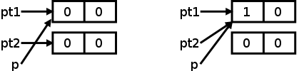
#include <stdio.h>
#include <stdlib.h>
class Point {
public:
  int x, y, w[2], *z;
  Point() : x(0), y(0) {
    w[0] = w[1] = 3;
    z = new int[2];
    z[1] = 9;
  }
};
int main(int argc, char *argv[]) {
  Point pt1, pt2;
  pt2 = pt1;
  printf("pt1: %d %d %d\n",pt1.x,pt1.w[1],pt1.z[1]);
  printf("pt2: %d %d %d\n",pt2.x,pt2.w[1],pt2.z[1]);
  pt1.x = 1;  pt1.w[1] = 5;  pt1.z[1] = 6;
  printf("pt1: %d %d %d\n",pt1.x,pt1.w[1],pt1.z[1]);
  printf("pt2: %d %d %d\n",pt2.x,pt2.w[1],pt2.z[1]);
  return 0;
}
    pt1: 0 3 9
  pt2: 0 3 9
  pt1: 1 5 6
  pt2: 0 3 6
C++: The C++ code
illustrates both value semantics and shallow copies.
To see the value semantics, just concentrate on the x field
in the Point class.
As in the Java code x is initialized to zero by the default
constructor.
The two points are simply declared, but with value semantics, this
declaration creates points (via the default constructor).
Assigning one to the other copies the point not the reference.
Hence we still have two points each referenced by one variable and,
therefore, changing the x component of one point does not
affect the other.
Note the addition of w and z to the class Point.
Each is in a sense an array of two integers (e.g., I print each
using array notation).
However z is heap allocated and the assignment of pt2
to pt1 results in only a shallow copy.
That is only the pointer is copied not the corresponding integers.
Thus changing pt1.z[1] changes the corresponding field of
pt2 as well.
Also, the heap space allocated in creating pt2.z is now
unreferenced and hence inaccessible.
Thus, we have leaked memory.
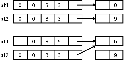
Homework:
CYU 23, 26 (ignore Eiffel and Smalltalk),
30 (substitute Java for Eiffel).
Start Lecture #11
9.4: Dynamic Method Binding
Referring back to the Point/ColoredPoint pair of classes, we see
that a ColoredPoint has all the properties of a Point (plus more).
So any place where a Point would be allowed, we should be allowed to
use a ColoredPoint.
Recalling Ada type terminology, the derived class acts like a
subclass of the base class.
Definition:
(Presumably) for this reason, the ability of a derived-class object
to be used where a base-class object is expected, is called
subtype polymorphism.
ColoredPoint *cp1 =
  new ColoredPoint (2.,3.,red);
Point *p1 = cp1;
p1->display();
Consider the code on the right.
We create a ColoredPoint pointed to by cp1 and declare a
Point pointer (sorry for the name) p1.
We initialize the second pointer using the first one.
This looks like a type mismatch, but is ok by subtype polymorphism.
The question is, Which display() method is invoked?
.
If the answer is Point.display() we have
static method binding.
This seems to be the right answer since after all the
type of p1 is pointer to
Point.
If the answer is ColoredPoint.display() we have
dynamic method binding.
This seems to be the right answer since after all the
object pointed to by p1 is a
ColoredPoint.
Semantics and Performance
Dynamic method binding does seem to have the preferred semantics.
The principal argument in its favor is that if the base-class method
is invoked on a derived object, it might not keep the derived object
consistent.
Performance considerations favor static method binding.
We shall see that dynamic binding requires each object to contain an
extra pointer and also
requires an additional pointer dereference when calling a method.
Language Choices
Smalltalk, Objective-C, Modula-3, Python, and Ruby use dynamic
binding for all methods.
Java and Eiffel use dynamic method binding by default.
This can be overridden with final in Java or
frozen in Eiffel.
Simula, C++, C# and Ada 95 use static method binding by default,
but permit dynamic method binding to be specified (see below).
9.4.1: Virtual and Nonvirtual Methods
In Simula, C++, and C# a base class declares as virtual
any method for which dynamic dispatch is to be used.
For example the move method of the Point class would be
written
virtual void move (double dx, double dy) { x += dx; y += dy; }
We shall see below how a vtable
is used to implement virtual
functions with only a small performance penalty.
Ada 95 uses a different mechanism for virtual functions that we
shall not study at this time.
class DrawableObject {
public:
  virtual void draw() = 0;
};
abstract class DrawableObject {
  public abstract void draw();
}
9.4.2: Abstract Classes
In most OO languages, it is possible to omit the body of a virtual
method in the base class, requiring that it be overridden in
derived classes.
A method having no body is normally called an
abstract method (C++ terms it pure virtual) and a
class with one or more abstract methods is called an
abstract class.
As shown on the right, C++ indicates an abstract method by setting
it equal to zero; Java (in my view more reasonably) labels both the
method and class abstract.
Naturally, no objects can be declared to be of an abstract class
since at least one of its methods is missing.
The purpose of an abstract class is to form a base for other
concrete classes.
Abstract class are useful for defining the API when the
implementation is unknown or must be hidden completely.
Classes all of whose members are abstract methods are called
interfaces in Java, C#, and Ada 2005.
Note that interfaces by definition contain no data fields.
9.4.3: Member Lookup
How can we implement dynamic method dispatch?
That is, how can we arrange that the method invoked depends on the
class of the object and not on the type of the variable?
The method to call at each point cannot be determined by the
compiler since it is easy to construct an in which the class of the
object referred at a point in the code depends on the control flow
up to that point.
Thus some run-time calculation will be needed and the method of
choice is as follows.
During execution a virtual method table (vtable) is
established for any class with one or more virtual methods; the
table contains a pointer for each of the virtual methods declared.
class B { // B for base
  int a;
public:
  virtual void f() {...}
  int          g() {...}
  virtual void h() {...}
  virtual void j() {...}
} b;
class D : public B {
  int w;
public:
          void f() {...}
  virtual void h() {...}
  virtual void z() {...}
} d;
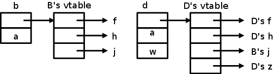
When a class is derived from this base class the derived vtable
starts with the base vtable and then
- Any overridden virtual methods have their entry point replaced by
the new method.
- Any additional virtual methods are added at the end.
When an object is created it contains a pointer to the vtable of
its class.
When a virtual method invocation is called for, we follow the
object's pointer to the class vtable and then follow the appropriate
pointer in the vtable to the correct method.
Converting Between Base and Derived Classes
#include <stdio.h>
class B {
public:
    int x;
    virtual void f() {printf("f()\n");}
} b, *pb;
class D : public B {
public:
    int y;
} d, *pd;
int main (int argc, char *argv[]) {
    B bl, *pbl;
    D dl, *pdl;
    printf ("main\n");
    b = d;
//  b = dynamic_cast<B>(d); not for objects
    b = (B)d;
//  d = b;   type error
//  d = dynamic_cast<D>(b); not for objects
//  d = (D)b; type error
    pb = &b;
    pd = &d;
    pb = pd;
    pb->x =1;
    pb = dynamic_cast<B*>(pd);
    pb->x =1;
    pb = (B*)pd;
    pb->x =1;
    pb = &b;
    pd = &d;
//  pd = pb;  illegal conversion
    pd = dynamic_cast<D*>(pb);
//  pd->y=1;   seg fault
    pd = (D*)pb;
    pd->y=1; // invalid, but no error msg
#include <stdio.h>
class B {
public:
    int x;
    virtual void f() {};
} b, *pb;
class D: public B {
public:
    int y;
} d, *pd;
int main(int argc, char *argv[]) {
    b.x = 11;
    d.y = 22;
    pb = &b;
    pd = (D*)pb;
    pd->y=1;
    printf("b.x=%d d.y=%d\n", b.x,d.y);
}
    pb = &d;
//  pd = pb;  type error
    pd = dynamic_cast<D*>(pb);
    pd->y=1;
    return 0;
};
C++:
On the right we see some C++ code that uses different methods to
convert between a base class B and a derived class D.
There are naming conventions to keep straight the properties of all
the variables.
- Variables containing a b in their name are declared to be in
the base class, a d signifies the derived class.
- If the name ends in b or d the declaration is global to the
main procedure that uses the variables; if the name ends in l it
is local to main.
Although both the local and global variables are declared, the
only uses shown are for the global.
I did compile and run the code with the local versions and the
results are the same.
- If the name begins with a p, the variable is a pointer to an
object; if the name does not begin with p, then it is an object
itself.
Note that the pointer declarations do not create
objects; the pointers are uninitialized.
Some of the lines are commented out.
These generated compile or run time errors as stated in the comment.
The version as shown compiles and runs.
The first set of attempted conversions tries to assign
dg to bg.
Recall that the first is a global variable containing an object of
the derived class and the second is a global variable containing an
object of the base class.
This is supposed to work (an object of the derived class can be used
where a base object is expected ) and indeed it does either naked,
as in the first line, or with an explicit cast as in the third.
The second line is an erroneous attempt to use for objects a feature
designed for pointers (see below).
Next we try the reverse assignment, which fails.
As expected, we cannot use a base object where a derived object is
expected.
Recall that the derived class typically extends the base so contains
more information.
Now we move from objects to pointers.
The first two lines initialize the pointers to appropriate objects
for their types.
Setting the base pointer to the derived pointer is legal: Since the
derived object can be considered a base object, the base pointer can
point to it.
Now the dynamic_cast is being used correctly.
It checks at run time if casting the pointer is type correct.
If so it performs the cast if not it converts the pointer to null
(which is type correct, but often leads to segmentation errors, see
below).
We also do the sometimes risky nonconverting type cast, which here
is type correct.
Next, we reinitialize the base and derived pointers to point to
base and derived objects and then try the invalid assignment of the
base pointer to the derived pointer, which would result in the
derived pointer pointing to a base object.
A naked assignment is caught by the compiler.
The dynamic cast does its thing and returns the null pointer, which
results in a segmentation fault when the pointer is used.
The nonconverting type cast works
, but the result is that the
derived pointer points to a base object, which has no y
component.
Although, assigning to t does not cause a error (this
time), it does not succeed in setting y.
Instead it must be setting some other word of memory; what a scary
thought!
This shows the danger of nonconverting type casts.
To illustrate that we have not set y, the next frame shows
a little test program.
When run, we find that setting y does not effect the value
of either y or x.
Finally we have the base pointer point to the derived object,
which is perfectly valid.
The subsequent naked assignment fails at compile time even thought
it is actually a legal assignment.
The dynamic_cast comes to the rescue.
The test program above, when modified for this case by changing
pb=&b;
to pb=&d;
(a one
character change) works fine and does indeed set y to 1.
public class B {
    public int a;
    public void f() {System.out.println("f()");}
}
public class D extends B {
    public int y,w;
    public void g() {System.out.println("g()");}
}
public class M {
    public static void main (String[] args) {
    B bg = new B();
    D dg = new D();
    System.out.println("main");
    bg = dg;
    bg = (B)dg;
    bg = new B();
    dg = new D();
//  dg = bg;  type error
//  dg = (D)bg; will not convert
    bg = new D();
//  dg = bg; type error
    dg = (D)bg;
    }
}
Java:
On the right we see a Java example.
Although shown here as one listing, each public class is actually a
separate .java file.
Java does not have C++ (really C) pointers so we don't use the
variables beginning with p as we did with the C++ example above.
But remember that, for objects, Java uses reference not value
semantics so all the variables are in a sense pointers; in
particular, an assignment statement changes the pointer not the
object.
The first group of statements shows that, as with C++, we can use a
derived object where a base is expected; the explicit cast is
optional.
In the second group we try to use a base class where a derived
class is expected.
Note that is this group the base variable refers to a base object
and the derived variable refers to a derived object (unlike the next
group).
The first line is a naked assignment and results in a compile time
type error.
In the second we employ a cast, which does compile (see the next
group), but then generates a run time error since a base object
cannot be viewed as a derived object.
The last group is perhaps the most interesting.
As before the derived variable refers to a derived object;
however, the base variable refers to a derived
not base object.
This is perfectly legal, for example, this is the state that
occurred after the first group of statements was executed.
It is still true that we cannot assign the base object to a derived
variable (type error) with a naked assignment.
However, the cast works because the error found in the second group
was via a dynamic, i.e., run time, check.
This time bg does refer (i.e., point) to a derived object and hence
the type can be converted and the assignment made.
More C++ vs Java: Terminology
| Java | C++ |
|---|
|
|
| Method | Virtual member function |
| Public/protected/private | Similar |
| Static Members | Same |
| Abstract methods | Pure virtual member functions |
| Interface | Pure virtual class with no data members |
| Interface implementation | inheritance from an abstract class |
fun mkAdder addend = (fn arg => arg+addend);
val add10 = mkAdder 10;
add10 25
class Adder {
  int addend;
public:
  Adder (int i) : addend(i) {}
  int operator() (int arg) { return arg+addend;}
};
int main (int argc, char *argv[]) {
    Adder f = Adder(10);
    printf("f(25)=%d\n",f(25));
    return 0;
}
Objects vs First-Class Functions
Using an Object to Produce a First-Class Function
Here is a clunky implementation of a simple first-class function
via an object.
The ML function mkAdder returns a function that adds the
given addend.
In the second frame we use mkAdder to produce
add10, which we use in the third frame (it gives an answer
of 35).
In the next frame is a C++ class that very cleverly does the same
thing.
It is tested in the next frame and the answer is again 35.
class Account { // Java
  private float theBalance;
  private float theRate;
  Account (float b, float r) {theBalance=b; theRate=r;}
  public void deposit (float x) {
    theBalance = theBalance + x;
  }
  public void compound () {
    theBalance = theBalance * (1.0 + rate);
  }
  public float balance () { return theBalance; }
}
(define Account
  (lambda (b r)
    (let ((theBalance b) (theRate r))
      (lambda (method)
    (cond
      ((eq? method 'deposit)
       (lambda (x) (set! theBalance (+ theBalance x))))
      ((eq? method 'compound)
       (set! theBalance (* theBalance (+ 1.0 theRate))))
      ((eq? method 'balance)
       theBalance))))))
Using a First-Class Function to Produce an Object
This time we are given a Java class that maintains a bank balance
and has methods for making a deposit, applying interest, and
retrieving the current balance.
When you create an instance of the class you give it an initial
balance and an interest rate to be applied whenever you invoke the
compound method (the name is chosen to suggest compound
interest).
The frame below gives a Scheme implementation using a function
Account that produces another function as a result.
It also uses two bangs.
Rather than give two more frames with the usage and answers, I
copied the file over to access.cims.nyu.edu so we can hopefully
see it work here.
9.4.4: Polymorphism
We will learn generics soon and have seen a
few hints already.
Some of the material from this section is discussed in our treatment
of generics.
The idea of generics is that you give a type variable as a parameter
of a generic and then instantiate the generic for various specific
types.
This is some times called
explicit parametric polymorphism as opposed to the
subtype polymorphism offered by inheritance.
Thus generics are useful for abstracting over unrelated
types, which is something inheritance does not support.
The Circle and the Ellipse: Subtype Polymorphism Gone Wrong
Every circle is an ellipse so it makes sense to derive a Circle
class from an Ellipse class and, by subtype polymorphism, to permit a
circle to be supplied when an ellipse is expected.
But this doesn't always work.
A reasonable method to have in the ellipse derived type is to
enlarge the ellipse by stretching it in two directions, parallel and
perpendicular to its major axis.
But if the two expansion coefficients are different a circle would
not remain a circle.
Homework: CYU 31, 32, 36 (only the C++ part), 37,
38.
9.5: Multiple Inheritance
9.6: Object-Oriented Programming Revisited
An interesting read; I recommend you do so.
9.A: Effective C++ (Scott Meyers)
class String {
private:
  char *data;
public:
  String(const char *value) {
    if (value) {
      data = new char[strlen(value) + 1];
      strcpy(data, value);
    }
    else {
      data = new char[1];
      *data = '\0';
    }
  }
  ~String() { delete [] data; \}
  ... // no copy constructor or operator=
};
String a("Hello");
{ // introduces a local scope
  String b("World");
  b = a;
}
String c = a;  // Same as   String c(a);
Meyers wrote two books (Effective C++ and
More Effective C++) that offer suggestions on a good C++
style.
I just show a very few, using material based on Prof Barrett's
notes.
Constructors, Destructors, and Assignment Operators
Item 11
Meyer's item 11
states
Declare a copy constructor and an assighment operator for classes
with dynamically allocated memory.
We saw an example previously, where the shallow copy performed by
the C++ default copy constructor, fails to copy dynamic memory.
It copies instead the pointer to the memory.
Look at the code on the right and notice that
- When b = a is executed, the string
World
is lost, a memory leak.
- When b goes out of scope, the string
Hello
is deleted, even though a still
contains this string.
- When c is constructed, using the default shallow copy
constructor, it also contains the deleted string!
- The
Hello
string may get deleted 3 times (the
effect of deleting an already-deleted string is undefined).
What is needed is a deep copy constructor that copies the string as
well as the pointer.
This is emphasized in lab 3.
#include <stdlib.h.>
class Vector {
private:
    int size;
    int *A;
public:
    Vector(int s) : size(s) {A = new int[size];}
};
class Array {
private:
    Vector data; // another class
    int size;
    int lBd, uBd;
public:
    Array(int low, int high) : lBd(low), uBd(high),
            size(high-low+1), data(size) {}
};
Item 13
Meyer's item 13
states
List members in an initialization list in the order in which they
are declared.
The code on the right is flawed.
The constructor for data will be passed an undefined value
because size has not yet been initialized, even though it
looks as though it has.
The reason is that members are initialized in the order they are
declared, not in the order they are
listed in the constructor.
So, to avoid confusion, when using an initialization list, you
should always list members in the order in which they are
declared.
int w, x, y, z;
w = x = y = z = 0
C& operator=(const C& rhs) {
  ...
  return *this;
}
Item 15
Meyer's item 15
states
Have operator= return a reference to *this.
The first frame is quite common in C and C++.
So you want to permit it for your classes, which is easy to do.
Just make sure that your operator= function returns
*this.
Item 16
Meyer's item 16
states
Assign to all data members in operator=.
If you don't have an operator=, C++ will do a shallow
assignment, which is fine for simple data like integers but not for
heap allocated data.
This is the reason you have operator=.
But, once you write operator=, C++ does nothing not even
the shallow assignment for items you don't mention.
So be sure to assign them all.
If this is a derived class, be sure to explicitly call the base
class operator= (this applies to the copy constructor as
well).
class My_Array {
  int * array;
  int count;
public:
  My_Array & operator = (const My_Array & other) {
    if (this != &other) // protect against invalid self-assignment {
      // 1: allocate new memory and copy the elements
      int *new_array = new int[other.count];
      std::copy(other.array, other.array + other.count, new_array);

      // 2: deallocate old memory
      delete [] array;

      // 3: assign the new memory to the object
      array = new_array;
      count = other.count;
    }
    // by convention, always return *this
    return *this;
  }
    ...
};
Item 17
Meyer's item 17
states
Check for assignment to self in operator=.
Since operator= will delete the old contents of the left
hand side, you must be check for the case where the client code is
simply x=x;.
Wikipedia gives a good fairly generic code example, which I copied
on the right.
Note that it makes sure to return *this
The principle followed is to proceed in this order
- Acquire new resources and copy needed value from old resources.
- Release old resources.
- Assign the new resources' handles to the object.
Start Lecture #12
Chapter 8: Subroutines and Control Abstraction (continued)
8.4: Generic Subroutines and Modules
What Is the Problem We Are Trying to Solve?
Think of a routine to sort an array of integers using heapsort.
Now imagine you need a routine to sort an array of
- Floats.
- Strings.
- Records containing two floats and an int.
The primary sort field is the int, but you break ties by looking
at the sum of the floats.
The sorting logic remains the same in all cases.
For the first three cases, you just want to change the type of some
variables from int to float to string
(assuming < for strings compares the strings not the addresses).
For the last case, you need to change the definition of < as
well.
Generics are good for this.
Generics are perhaps most widely used for
containers, structures that contain items, but
whose structure doesn't depend on the type of the items contained.
Examples include, stacks, queues, dequeues, etc.
Normally, the containers are homogeneous, that is, all of the items
in a given container are of the same type.
We don't want to re-implement the container for each possible item
type.
Why Isn't Inheritance Good Enough?
Inheritance is also used for containers, indeed, containers formed
one of our chief inheritance examples (lists, queues, and dequeues).
The the comments that follow are inspired by words in section 9.4.4
(part of the chapter on inheritance).
I deferred it to here since we did inheritance before generics so
could better compare the two when doing generics.
When studying inheritance, we considered a gp_list_node
class and derived from that int_list_node,
float_list_node, etc.
This seemed pretty good since all the list properties (predecessor,
successor, etc) were defined in the gp_list_node class and
thus inherited by each *_list_node class.
int_list_node *q, *r;
...
r = q->successor();  // error: type clash


gp_list_node *p = q->successor();
cout << p.val;       // error: gp_list_nodes have no val


r = (int_list_node*) q->successor();
cout << r.val              // OK, but scary


r = dynamic_cast<int_list_node*> q->successor()
cout << r.val              // OK if have vtable


int_list_node* successor() {
  return (int_list_node*) gp_list_node::successor();
}
However, problems remain.
The first frame represents what I would consider natural code for
marching down a list built of int_list_nodes.
It fails because successor() returns a
gp_list_node*, which cannot be nakedly assigned to an
int_list_node*.
The second frame shows the result of quickly applying the motto
fix it now; understand it later
.
The third frame shows a real fix.
However, a nonconverting type cast is always scary.
The fourth frame also gives a real fix; one that is not so scary.
However, it wouldn't work for the specific code we had since there
were no virtual functions and hence no vtable.
We certainly could have added a virtual function and, more
importantly, a large project would very likely have one.
Clients of our class would not be happy with this awkward solution
and hence we would likely revise int_list_node
to redefine
successor() as shown in the next frame.
This last solution seems the best of the possibilities, but is far
from wonderful since we needed to redefine methods whose
functionality did not change.
We have lost some of the reuse advantages of inheritance!
template<class V>
class list_node {
  list_node<V>* prev;
  list_node<V>* next;
  list_node<V>* head_node;
public:
  V val;
  list_node()  // SAME code as in orig
  list_node<V>* predecessor() { // SAME code as in orig
    if (prev == this || prev == head_node) return 0;
    return prev; }
  list_node<V>* successor() {...}
  void insert_before(list_node<V> new_node) {...}
    ...
};
template<class V>
class list {
  list_node<V> header;
public:
  list_node<V>* head() {...}
  void append(list_node<V> *new_node) {}
  ...
};
typedef list_node<int> int_list_node;
typedef list<int> int_list;
...
int_list numbers;  // list<int> without typedef
int_list_node *p;
...
p = numbers.head();
...
p = p->successor();  // no cast required!
The Solution with Generics
On the right we see the solution with generics.
The classes list_node and list have been
parameterized with the type V.
Think of instantiating this with V=int and then
instantiating it again with V=float.
With V=int we see that the first public field becomes
int val, which is perfect (i.e., is exactly what it
was for int_list_node previously).
The prev field is of type list_node<int>*,
which is reasonably close to int_list_node.
In order to permit the clients to use int_list_node, they
need only include a typedef as we have done.
Finally, note that the code to march down a list is the natural
linked list code.
All in all this use of generics turned out quite well.
Back to the Present (section 8.4)
Having shown by an example that inheritance, which we have already
studied, does not by itself eliminate the need for generics, we turn
our attention to a proper treatment of generics itself.
We just looked at a linked list example where the type of the data
items (the val field) can vary.
For now just think of int and float.
If we were to explicitly declare the data item, as is needed in
languages like Pascal and Fortran, then we would need separate
routines for ints and floats.
The difficulty is not in producing the multiple versions (copy/paste
does most of the work), but rather in keeping them consistent.
In particular, it is a maintenance headache to need to remember to
apply each change to every copy
.
We could have the lists contain pointers to the data item rather
than the items themselves (cf. reference vs.
value semantics).
This would be the likely solution in C.
Of course a pointer to an int, i.e., an int* is
not type compatible with a float*, so we play the merry
game of casts and kiss off the advantages of compile time type
checking.
An alternative in C is to use the macro facility to produce all the
different versions.
As we have seen when studying
call-by-name, macro expansion requires
care to prevent unintended consequences.
We could use implicit parametric polymorphism as we have seen in
Scheme and ML.
The disadvantage of the Scheme approach (shared with many scripting
languages) is that type checking is deferred to run time.
ML is indeed statically typed, but this does cause the compiler to
be substantially slower and more complicated (not noticeable for the
tiny programs we wrote).
Moreover, ML has been forced to adopt structural type equivalence
instead of the currently favored name equivalence.
Finally, we saw early in the course that ML's treatment of
redeclaration differs from that chosen
by most languages supporting the feature.
Models Used for Generics in Various Languages
| Language | Model |
|---|
| C | Macros (textual substitution) or unsafe casts |
| Ada | Generic units and instantiations |
| C++, Java, and C# | Templates |
| ML | Parameteric polymorphism, functors |
In this section we will study explicit polymorphism in the
form of generics (called templates
in C++).
The different models used for generics are summarized in the table
on the right.
A Little History for Ada, C++, C#, and Java Generics
Ada generics were in the original design and Ada 83
implementations included generics.
Generics were envisioned for C++ early in its evolution, but only
added officially in 1990.
C# generics were also planned from the beginning but didn't appear
until 2004 (release 2.0).
Java, in contrast, had generics omitted by design;
they were added (to Java version 5) only after strong demand from
the user community.
Parameterizing Generics
As we have stated a generic facility is used to have the
same code apply in a variety of different circumstances.
In particular, it is to be applied for different values of the
parameters of the generic.
These parameters are called the generic parameters.
Let first consider a simple case.
If we had a generic array, the natural parameters would be the array
bounds and the type of the components.
Indeed the definition of a (1-dimensional, constrained) array in Ada
is of the form
<array_name> : array <discrete_subtype> of <component_type> ;
The discrete subtype is characterized by its bounds.
Higher dimensional arrays simply have more
<discrete_subtypes>.
(Ada also has unconstrained array types, that we are not discussing).
So for a given array declaration, we supply the index bounds and
the type of the components; these are the parameters.
An (ordinary) subprogram is also generic in that it can be applied
to various values for its arguments; those arguments are the
parameters.
Parameters for Various Generic Facilities (incomplete).
| Construct | Parameter(s) |
|---|
| array | bounds, element type |
| subprogram | values (the arguments) |
| Ada generic package | values, types, packages |
| Ada generic subprogram | values, types |
| C++ class template | values, types |
| C++ function template | values, types |
| Java generic | classes |
| ML function | values (including other functions) |
| ML type constructor | types |
| ML functor | values, types, structures |
In all cases it is important to distinguish the parameters from the
construct being parameterized.
For example, we parameterize a subprogram by supplying
values as parameters.
Turning to the new constructs, we see that in many cases types can
be parameters.
So an Ada generic subprogram for sorting would take a type parameter
and thus can serve as an integer sorter, a float sorter, etc.
There is a weird (mis)naming convention you should understand and
sadly must deal with.
Recall from above the C++ phrase
template<class V>.
The requirement is that V must be a type.
Moreover, there is an alternative syntax
template<typename V> that is perfectly legal and
completely descriptive.
However, probably from habit, it is not normally used.
I found a clear explanation
here.
generic
   type T is private;
procedure swap (A : in out T; B : in out T);
procedure swap (A: in out T; B : in out T) is
   Temp : T;
begin
   Temp := A; A :=B ; B := Temp;
end swap;
with swap;
procedure Main is
   procedure SwapInt is new Swap(Integer);
   X : Integer := 3;
   Y : Integer := 4;
begin
   SwapInt(X,Y);
end Main;
A Generic Swap in Ada
On the right is the familiar three part Ada example: specification,
body, use.
We offer to clients a generic procedure Swap; the
genericity is parameterized by a type T (private is
explained below).
The body implements Swap, which is trivial.
Note that here the type T is treated as a normal type.
The client instantiates a new procedure SwapInt, which is
the generic Swap, with the generic class T replaced by the
specific class Integer.
The instantiated procedure SwapInt is used just as if it
were defined normally.
What about the private in the specification?
The purpose of this private (or of other possibilities) can
be seen from two viewpoints: the client or the author of the body.
From the author's viewpoint, private is saying what
properties of T can be used.
The private classification means that variables can be
declared of type T and can be assigned and compared for
equality.
No other properties can be assumed.
For example, the author cannot ask if one type T value is
less than another (so we couldn't write a maximum function).
A more restrictive possibility would be limited private in
which case assignment and equality comparison are forbidden as well.
So, from the author's viewpoint, the more restrictive the
requirement, the less functionality is available.
The more the author is constrained, the less the
client is constrained since whatever functionality the author
can assume about type T, the client must
guarantee his specific type supplies.
generic
   type T is private;
   with function ">" (X,Y : T) return Boolean;
function max (A,B : T) return T;
function Max (A,B : T) return T is
begin
   if A > B then return A; end if;
   return B;
end Max;
with Max;
procedure Main1 is
   function MaxInt is new Max(Integer,">");
   X : Integer;
begin
   X := MaxInt(3,4);
end Main1;
A Generic Max in Ada
As just mentioned, the generic type parameter cannot, by default,
be assumed to supply a > operator.
So to implement a generic max, we need to pass in the > as a parameter.
The first frame again has the specification.
We see that the second generic parameter is >.
Don't read too much into with; it is there to prevent a
syntactic ambiguity.
Frame 2 is a standard maximum implementation.
In the last frame we see that we are supplying > for >.
Since this is so common, there is extra notation possible in the
specification to make it the default.
In any event, when MaxInt is instantiated the compiler checks to see
that there is a unique operator visible at that point that matches
the signature in the specification.
As a not-recommended curiosity, I point out
function MinInt is new Max(Integer, "<");
generic
   MaxSize: Positive;
   type ItemType is private;
package Stack is
   procedure Push(X: ItemType);
   function Pop return ItemType;
end Stack;
package body Stack is
   S: array(0..MaxSize-1) of ItemType;
   Top: Integer range 0..MaxSize;
   procedure Push(X: ItemType) is
   begin
      S(Top) := X;
      Top := Top+1;
   end Push;
   function Pop return ItemType is
   begin
      Top := Top-1;
      return S(Top);
   end Pop;
begin
   Top := 0;
end Stack;
with Stack;
procedure Main2 is
   package MyStack is new Stack(100,Float);
   X: Float;
begin
   MyStack.Push(6.5);
   X := MyStack.Pop;
end Main2;
A Generic Stack Package in Ada
Here we see a generic parameter that is not a type.
The parameter MaxSize is a value, in this case a positive
integer.
The third possibility in which a package is a parameter to another
package is not illustrated.
The specification has the generic prefix and then looks like a
stack package.
It offers the standard push and pop subroutines.
The MaxSize parameter is not used here; it is needed in the body.
The package body is completely unremarkable.
Indeed, if you just substitute some positive value for MaxSize and
some type for ItemType, it is a normal stack package body.
It can certainly be criticized for not checking for stack overflow
and underflow.
The client code is also not surprising, but does have a curiosity.
MyClient.Push looks like OOP.
It isn't really since MyClient is a package not an object, but it
does look that way.
Indeed, you could remove both generic parameters, changing the
specification and body to use say 100 and float and still
create several new packages MyStack1,
Mystack2, etc.
Then you would have MyStack1.Push(5.2);,
X:=MyStack2.pop;, etc.
template<typename itemType, int maxSize>
class stack {
     int top;
     itemType S[maxSize];
public:
     stack() : top(0) {}
     void push (itemType x) {
         S[top++] = x;
     }
     itemType pop() {
         return S[--top];
     }
};
#include <iostream>
#include "stack.cpp"
int main(int argc, char *argv[]) {
     stack<float, 50> myStack;
     float x;
     myStack.push(4.5);
     x  = myStack.pop();
}
The Same
Generic Stack Package in C++
On the right is the C++ analogue of the Ada stack package above.
The first frame is the body (implementation), the specification
(interface) is not shown.
The C++ body is clearly much shorter than the Ada version.
The only functionality missing is the range specification for
Top; the real reason the lengths are so different is the
relative emphasis the two languages place on readability vs
conciseness.
The client code in the next frame is almost the same as the Ada
version.
public class Stack<T> {
  final int maxSize;
  int top;
  T[] S;
  public Stack(int size) {
    maxSize = size;
    top = 0;
    S = (T[]) new Object[maxSize];
  }
  public void push(T x) {
    S[top++] = x;
  }
  public T pop() {
    return S[--top];
  }
}
public class MainClass {
  public static void main(String args[]) {
    Stack<Float> myStack = new Stack<Float>(10);
    Float X;
    myStack.push(3.2F);
    X = myStack.pop();
  }
}
The Same
Generic Stack Package in Java
There is a difference in the Java implementation.
The generic parameters must be classes; in particular the integer
maxSize cannot be specified as a generic parameter.
Instead we pass the size as an argument to the constructor.
Also, as usual, the reference semantics of Java means that declaring
a stack only gives a reference so we need to call new.
The biggest change is that Java does not permit us to say
new T so we must produce an Object and cast
it to T using an unsafe cast.
The client code has a change as well.
Note the capital F in Float; this is a class, rather that
the primitive type float, which would be illegal.
An experienced Java programmer would use a different implementation.
public class Stack<T> {
   readonly int maxSize;
   int Top;
   T[] S;
   public Stack(int size) {
      maxSize = size;
      top = 0;
      S = new T[m_Size];
   }
   public void Push(T x) {
      S[top++] = x;
   }
   public T Pop() {
         return S[top--];
   }
}
public class MainClass {
  public static void Main(String args[]) {
    Stack<float> myStack = new Stack<float>(10);
    float X;
    myStack.push(3.2F);
    X = myStack.pop();
  }
}
The Same
Generic Stack Package in C#
C# looks
like Java, but there are differences.
In a sense C# is between
C++ and Java.
The keyword final has become readonly and, in the
client code, Main is capitalized.
These are trivialities.
Much more significantly two of the Java quirks are missing.
We now write new T directly, eliminating the unsafe cast
and the client can use the primitive type float rather than
a class that acts as a wrapper (and increases overhead).
Summary
In summary, we can say that for simple cases like the above stack,
the C++, C#, Java, and Ada solutions are basically the same from the
programmer's viewpoint (with the exception of no primitive types or
new Tin Java).
We shall see that the implementations are different.
8.4.1: Implementation Options
In Ada and C++, each instantiation of a generic is separate.
So
stack<float,50> myStack1 and
stack<int,50> myStack2
will likely not share code for the push and pop
routines.
Indeed it is not clear if two instantiations with the
same generic parameters will share code.
This rather static approach may look similar to a macro expansion as
for example in C.
However
- Generics are integrated into C++ and Ada; they don't give the
appearance of a late addition as do C macros.
- Generic parameters are type checked.
- Arguments to a generic routine are evaluated exactly once.
That is they use the same applicative order semantics found in
the rest of the language.
C macros are much more call-by-name like and the arguments are
evaluated each time they are used in the macro.
- Names inside generics obey the normal language scoping rules.
In contrast to the separate instantiation characteristic of C++ and
Ada, all instantiations of a given Java generic will share
the same code.
One reason this is possible is that, due to its reference semantics,
all the elements are of the same size (a pointer).
Another reason is that only classes, and not primitive types or
values, can be used as generic parameters.
In the next section, we will see that the strong compatibility
requirements of Java have limited the power of its generics
facility.
The C# language, like Java, has much code sharing, but without the
limitations caused by Java's type erasure
implementation
described below.
C# does permit primitive types as generic parameters.
A C# generic class does share code between all instantiations using
classes as parameters (the only possibility for Java), but produces
specialize code for each primitive type instantiated.
As with Java, the C# generic parameters must be types, not values.
Java Type Erasure
The designers of Java version 5 very much wanted to maintain strong
compatibility with previous versons of Java that did not include
generics.
Indeed, the compatibility requirements were not only that legacy
Java would run together with Java 5 code, but also that the JVM
would not need to change.
As a result they implemented generics using
type erasure.
The idea of type erasure is, as the name suggests, that the generic
type is, in essence, erased from the generic class.
First, the compiler removes the <T> from the header.
Then all occurrences of T in the generic body are replaced
by object, the most general class in Java.
Finally, the compiler inserts casts back to T whenever an
Object is returned from a generic method.
These casts are reminiscent of the best
of the non-generic
solutions for a linked-list that we discussed
previously.
A significant advantage of type erasure over the non-generic
solution is that the generic-routine programmer does not have to
write the casts and the generic-routine reader does not have see
them.
Type erasure has its own disadvantages.
For example, a Java Class C<T> cannot
execute new T.
This is a serious limitation, but the Java 5 designers felt that the
resulting strong compatibility was worth it.
Another consequence of type erasure is that C<T1>
and C<T2> do not produce different types.
Instead, they both yield the raw
type Gen.
The above discussion assumed only one generic parameter.
However, multiple generic parameters are permitted and the
comments made generalize fairly easily.
C# Reification
First, for those like me who didn't know what reify meant the
definition from the Webster online dictionary is
to regard (something abstract) as a material or concrete thing
.
In C# each instantiation of Class C<T> with a
different T yields a distinct type.
I suppose this matches the definition of reification by having
the something abstract
be the parameterized type and having the
concrete thing
be the new, distinct type.
With each instantiated type (having distinct generic parameter
values) as a different type, C# reification does not lead to the
restrictions mentioned above for type erasure.
(Don't forget that, in legacy Java, generics were
omitted by design
and the Java 5 implementers had extremely
strong compatibility constraints.)
generic
   type T is private;
   with function "<"(X,Y:T) return Boolean;
function Smaller (X,Y:T) return T;
function Smaller (X,Y:T) return T is
begin
   if X<Y then return X; end if;
   return Y;
end Smaller;
with Smaller;
with Ada.Text_IO; use Ada.Text_IO;
with Ada.Integer_Text_IO; use Ada.Integer_Text_IO;
with Ada.Float_Text_IO; use Ada.Float_Text_IO;
procedure Main is
   type R is record
      I: Integer;
      A,B: Float;
   end record;
   R1: R := (1, 0.0, 0.0);
   R2: R := (1, 2.0, 3.0);
   R3: R;
   function "<"(X,Y:R) return Boolean is
   begin
      if X.I < Y.I then return True; end if;
      if X.I > Y.I then return False; end if;
      return (X.A+X.B)<(Y.A+Y.B);
   end "<";
   function SmallerR is new Smaller(R,"<");
begin
   R3 := SmallerR(R1,R2);
   Put ("The smaller is: ("); Put (R3.I);
   Put (", "); Put(R3.A);
   Put (", "); Put(R3.B);
end Main;
8.4.2: Generic Parameter Constraints
Let us restrict attention to the case of just one generic parameter
as the generalization to multiple parameters is straightforward.
Also, let us consider only the case of a type parameter
since those are permitted in all the languages (in Java the type
must be a class not a primitive type).
Generic Parameter Constraints in Ada
Recall that the Ada generic Stack package began
    generic
        MaxSize: Positive;
        type ItemType is private;
    package Stack is
and recall that a private type can only be assumed to support,
assignment, equality testing, and accessing a few standard
attributes (e.g., size).
In place of private a few other designations can be used,
but they do not come close to giving all useful restrictions on (or,
equivalently, requirements of) the type.
We mentioned using with to add other requirements on the
type and mentioned that, given the appropriate definition, we could
compare records containing one integer and two floats, by first
comparing the integers and, if there is a tie, comparing the sum of
the floats.
On the right is an implementation, in the usual three-part Ada
style.
Note, in particular the overload resolution of <
in the
instantiation of the generic Smaller into the specific
SmallerT.
Generic Parameter Constraints in C++
The C++ generic programmer can omit explicit constraints and write
a header as simple as
    template<typename T>
    void sort(T A[], int A_size) {...}
Then, when the generic component is instantiate, the compiler checks
to ensure that the supplied type has all the properties used in the
generic body.
This is certainly concise, but does sacrifice clarity in that users
of the generic component, must themselves ensure that the type they
supply has all the needed properties.
Worse, the type supplied might indeed supply the property, but the
default property may not do what the user wanted and expected.
For these reasons, many users shun implicit constraints and make
the requirements explicit.
The Ada technique above can be employed: the comparison operator can
be specified as a method of type T.
However, rather than needing to explicitly list all the operators
needed, the Java/C# method below can also be used in C++.
Generic Parameter Constraints in Java and C#
Java and C# make use of inheritance to specify the needed
constraints for generic parameters.
A good example is sorting
public static <T extends Comparable<T>> void sort(T A[]) {
This generic header says that the sort routing will use
type T and that T is required to have all the
methods found in the Comparable interface.
(Recall that an interface has only virtual methods).
In this case Comparable is a Java standard interface and
contains CompareTo, which compares two values returning -1,
0, +1 for the three cases of <, =, and >.
The generic sort routine then contains a line like
if (A[i].compareTo(A[j]) ≥ 0)
which holds precisely if, according to type T,
A[i]≥A[j].
In other examples the interface the parameter T
extends, will be user defined and will contain several
virtual functions, all of which any type used to instantiate
T is required to have.
C# has the same concept, but with slightly different syntax.
8.4.3: Implicit Instantiation
All four languages we studied require explicit
instantiation for generic packages/classes.
However, they differ for generic routines.
In Ada, a generic routine must be explicitly instantiated.
Our most recent Ada example illustrated the instantiation of the
generic routine Smaller into the specific routine
SmallerR by replacing the generic type T with the specific
type R.
In contrast C++, C#, and Java use
implicit instantiation.
That is they treat the generic version as an overloaded name that is
resolved at usage.
Thus after writing a generic sort routine, the programmer
simply invokes it with arguments of type R and the system
automatically (implicitly) instantiates a concrete version for type
R (and for C# and Java has it share code with other instantiated
versions).
8.4.4: Generics in C++, Java, and C#
Some of the material from this section (including the CD portion)
has been incorporated in the above.
The rest is being omitted.
8.A: Generics in ML
ML generics are called functors (a term from mathematics).
You might ask, given the parametric polymorphic functions for
which ML is justly famous, and also the type constructors, which
we have not seen, why are generics needed at all?
- Functors can take structures (ML modules) as
arguments, which is not possible for functions or type
constructors.
- Sometimes we want to parameterize a type with a value, which
is not possible using type constructors.
8.B: Iterators and the C++ Standard Template Library STL
Iterators are entities used for accessing (iterating over) the
elements of a container (list, array, tree, queue, etc).
The C++ STL is a large collection of generic classes used mostly for
containers.
It also provides a large collection of Iterators.
The STL makes little use of inheritance.
Homework: CYU 27, 29, 30, 31.
Homework:
Using the code in the notes for section 8.4.2,
produce a generic sort in Ada (a trivial
O(N2) sort, like bubble sort is fine).
Instantiate it to sort type R items using the
integer as the primary key and the sum of
the floats to break ties.
Start Lecture #13
8.5: Exception Handling
Definition: An exception is
unexpected/unusual condition that can arise during program
execution, and that cannot be handled easily in the local context in
which it occurs.
Broadly speaking exceptions come in two categories.
- Predefined exceptions are detected
automatically by the language runtime system.
Examples include
- Constraint violations (exceeding array bounds, dividing by
zero, etc).
- I/O conditions (end of file—EOF— encountered,
ill-formed numerical input, insufficient privilege, etc).
- Insufficient memory for allocation.
- User defined exceptions are raised
explicitly by the program.
When we studied modules, the better
Ada queue implementation
included QueueFull and QueueEmpty exceptions
that were defined in the code and explicitly raised when the
appropriate conditions occurred.
The programmer writes exception handlers (for
either predefined or user-defined exceptions).
The handler is invoked when the exception is raised and can specify
remedial action or can orchestrate an orderly shutdown.
Exceptions can be stored and re-raised later.
Handling Errors
Of course good programs check for possible errors.
What should we do when we find an error (EOF when looking for data;
non-existent file when attempting an open, etc)?
- We could return a special value that the caller checks for,
in place of a normal returned value.
- Return an extra
status
value.
This is conceptually similar to the first solution.
- Have the caller pass a closure that is to be invoked in case
of an error
The first two are not lovely; the third is discussed at the end of
this lecture (Scheme continuations
).
- It is easy for the caller to forget to make the check.
- The check clutters up the normal case of the code.
Indeed with enough checks it is hard to see what the normal case
is.
Presumably, the normal, error-free case is the most common.
Exception mechanisms incorporated in the language aid the
programmer in producing clear code and ease the task of catching
errors.
When an exception occurs in a monitored block of code, the
handler for that exception is invoked and is
executed instead of the yet-to-be performed portion of the
monitored block.
What Do Handlers Do?
Typically a handler does one of three things.
- Ideally a handler, will compensate for the exception so that
the program can recover and continue.
Below we see an Ada program that
recovers
from bad input
by printing a message and having the user re-input the value.
- If the local block cannot recover, it should clean up its
local action and re-raise the exception so that it will
propagate back the dynamic chain to a handler
that can recover.
- If the exception cannot be repaired at all, at least a helpful
message, possibly plus data, can be printed to help in debugging.
Why the Dynamic (not Lexical) Chain?
The reason the exception propagates back the dynamic chain rather
that going to a higher lexical scope is that exceptions are runtime
phenomena and it is the dynamic execution that produced the values
causing the exception.
8.5.1: Defining Exceptions
Some Generalities
We have seen/will see examples of exceptions being triggered and
being caught in Ada, C++, Java, and ML.
In all cases there are three parts to the exception handling
mechanism.
- A lexical region of the program.
- A specific list of
exceptional conditions
.
- A set of actions.
If one of the exceptional conditions occurs while the program is
executing the indicated region (or other code invoked—directly
or indirectly—by this region), then control transfers to one
of the specified actions.
When the chosen action completes control returns to the
end of the indicated region.
In the better Ada queue example, the lexical
region is a begin block with three queue operations and a simple
if-then-else statement, the exceptional conditions are the
QueueFull and QueueEmpty conditions, and the
action list consists of two Put_Line instructions.
Although, neither QueueFull nor QueueEmpty can
be triggered by any statement in the begin block, both can occur
while executing the queue operations invoked in the begin block.
Defining Exceptions in Ada
As mentioned above, the exceptional conditions can be predefined in
the language or user-defined by the programmer.
Ada 95 has four predefined exceptions that are declared in the
package Standard, all of which indicate that
something has gone seriously wrong.
- Constraint_Error: Some value is out of range, which
includes a value not in the domain of an operation (e.g, a
divisor of zero).
- Program_Error: An attempt to violate the control
structure has occurred (and has not been detected at compile
time).
For example if a Function reaches the end
without hitting a return statement.
- Storage_Error: The system has run out of space.
- Tasking Error: Some problem with concurrency.
In addition the package Ada.IO_Exceptions defines eight
more: Status_Error, Mode_Error,
Name_Error, Use_Error, Device_Error,
End_Error, Data_Error, and Layout_Error.
Nearly all represent error conditions, only End_Error,
which indicates that an input instruction has encountered an end of
file, can be considered an expected occurrence.
We shall see that Ada is unusual in that the raise
statement gives the handler no information other than the exception
name.
Other languages permit additional data to be passed to the handler
as a parameter.
In Ada, the handler itself can obtain other information, as we show
below.
Moreover, instead of the simple raise statement the
programmer can employ raise_exception, a procedure that
permits more information to be sent to the handler.
with Ada.Integer_Text_IO; with Ada.Text_IO;
use Ada.Integer_Text_IO; use Ada.Text_IO;
function Get_Data return Integer is
  X: Integer;
begin
  loop
    begin
      Get(X);
      return X;
    exception
      when others =>
        Put_Line("Need integer; try again.");
    end;
  end loop;
end Get_Data;
Builtin Exception Example—Checking Input Data:
The simple example on the right illustrates a few points about
exception handling in Ada.
- The keyword others, which matches any exception.
Actually, it would be better use the exact exception,
Data_Error in this case, and save others for
unexpected exceptions.
- The extra begin block added just to handle the
exception.
(loop...end loop does not require a begin).
- The flow of control caused by an exception.
The handler executes instead of the remainder of the
begin block.
So, in this case, if the input is bad, the return is
not executed.
Note that the exception essentially completes the begin
block and hence the next iteration of the loop does
execute, as desired.
User-Define Exception Example:
We have already seen user-defined exceptions in Ada when we
wrote the better queue example.
After reviewing that example, we should note the following points
about the use of exceptions.
The example asserts that we have declared
two exceptions.
This is not strictly true as exceptions are not members of a type:
for example, there are no exception variables.
when Event: others =>
  Put("Unexpected Exception: ");
  Put(Exception_Name(Event));
  New_Line;
  Put(Exception_Message(Event));
  raise;
end;
However Ada has a related concept,
Exception_Occurrence, which is a type.
Consider the code fragment on the right.
The variable Event is called a choice parameter
.
A variable declared in this unusual way is of type
Exception_Occurrence and contains a great deal of
information about the exception that has just occurred.
The code uses two system-supplied functions that accept as
arguments variables of this type.
Another such function is Exception_Information, which
unlike the one-line Exception_Message, gives details,
sometimes including a trace back.
An Exception_Occurrence, including all its information, can
be saved using other procedures and functions.
The package Ada.Exceptions has all the machinery.
Another point shown in the code is the raise statement
used without an exception name.
This usage re-raises the same exception in the dynamically previous
scope.
try {
  ...
  if (...) throw 8;
  ...
}catch (int e){
  cout<<"caught "<< e <<"\n";
}
#include <iostream>
class zerodivide {
public:
  zerodivide() {}
};
int main (int argc, char *argv[]) {
  try{
     throw zerodivide::zerodivide();
  }catch(zerodivide z){
    std::cout<<"caught";
  }
}
Defining Exceptions in C++
Although the runtime time behavior is similar (exceptions are
raised and caught), C++ and Ada do have real differences in exception
handling.
One difference is that exceptions are only raised explicitly by a
throw statement; there is no analogue of the Ada builtin
exceptions.
Flash: Apparently, there is at least one builtin
exception namely bad_cast, which is thrown by our friend
dynamic_cast<T>, when the type T is a
reference (we have used it only when T was a pointer, in
which case it does not throw an exception).
As the top example on the right illustrates, the Ada begin
block becomes a try block in C++; raise becomes
throw; and when becomes catch.
However, the details differ significantly.
In Ada you declare
exceptions and raise them.
In C++ you throw any object; the top example on the right
throws an integer.
Throw and catch act a little like a subroutine
call in that the object thrown becomes the parameter of the
catch.
Often you declare a unique class for each type of exception you
wish to throw; the second example shows the class
zerodivide.
Note that nothing in the class associates it with exception
handling.
Since we do not have an object of class zerodivide
available, the throw in this case is a call to the
constructor, which produces the needed object.
It is common usage in cases like this where the parameter
z is not used in the catch for it to be omitted
and the line to the right is replaced by
}catch(zerodivide){.
A catch statement for a class C also catches throws of any
object in a class D derived from C.
Although both our examples had only one catch block for
each throw block, one can have multiple catches.
In that case the first one that matches is chosen.
Thus, if you have a catch for class C and another
catch for class D derived from C, you must place
the catch for D first (otherwise D exceptions would be
caught by the C handler).
The most general catch statement possible is written
catch(...) and will catch any exception.
Another difference between Ada and C++ exceptions is that C++
exceptions are bona-fide types.
A subroutine header in C++ can optionally include a list of
exceptions that may propagate out of the subroutine.
If the list does appear and an exception occurs that is not caught
locally, the program is terminated.
If the list does not appear, all exceptions not caught locally will
propagate.
Compare this with the Java behavior described below.
public class Zd extends Exception {
  public Zd() {};
  public static void main(String[] args) {
    try{ ...
      if (...) throw new Zd();
    }catch(Zd z){
      System.out.println("caught");
    }
  }
}
Defining Exceptions in Java
The Java model is close to C++ as seen by the example on the right
with its try. throw, and catch.
But of course there are differences.
Checked and Unchecked Exceptions:
Java makes an important distinction between
checked and unchecked exceptions.
The basic idea is that the program should be aware of checked
exceptions, and either handle them if they occur or announce their
possibility to callers of the method.
Unchecked exceptions are those from which it is not reasonable to
expect the program to recover and methods are permitted to ignore
the possibility of their occurring.
This distinction is specified via the class hierarchy as follows.
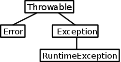
All classes that are thrown and caught, must be subclasses of the
system class throwable, which has derived classes
Exception and Error.
The former has a derived class RuntimeException
- Classes extending Error are unchecked
exceptions.
- Most classes, such as my Zd, that extend Exception
are checked exceptions and must either be handled (with
a catch) or declared in the method header
- Classes that extend RuntimeException are
unchecked.
import java.io.*
public void f() throws FileNotFoundException {
  FileInputStream fis =
   new FileInputStream("/tmp/x");
}
The method f on the right needs the throws clause
because the constructor for FileInputStream can throw the
checked exception FileNotFoundException and hence
f must either catch that exception or
announce it in the header as I did.
Failure to do so would result in a compile time error.
exception DivideByZero
fun f (i,j) =
    if j = 0
    then raise DivideByZero
    else i div j;
f(6,2) handle DivideByZero => 42;
f(6,0) handle DivideByZero => 42;
- [opening /tmp/handle.sml]
exception DivideByZero
val f = fn : int * int -> int
val it = 3 : int
val it = 42 : int
Defining Exceptions in ML
Again the runtime model is similar, but with differences.
Perhaps the major difference is that ML is an expression language so
a handle is attached to an expression and
the handle itself must return a value of the same type as the
expression it is attached to.
On the right is a simple example.
It is possible for the exception statement to have
parameters, in which case the corresponding raise statement
must supply arguments.
8.5.2: Exception Propagation
As we have seen, when an exception occurs, the local handlers are
checked in order and control is transferred to the first one that
matches (remember that a handler for a C++ or Java class also
handles exceptions of any derived class).
If the local environment doesn't catch an exception, in most cases
it propagates back up the dynamic chain to the caller.
The exception is that, if a C++ routine lists exceptions that can
propagate, and a different exception arises and is not caught
locally, then the program terminates.
If the exception propagates to a routine outside the scope of the
exception declaration, then the exception cannot be named and hence
can be caught locally only with a catch-all
statement.
Typically, if an exception propagates all the way out of the main
program, the job terminates.
A question arises what to do with a multi-threaded job if one of the
threads has an exception propagate all the way out.
In Ada and Java, just the thread terminates; in Modula-3, the entire
job terminates; and C++ does not specify.
Handlers on Expressions
As we have seen above, expression languages like ML attach
exception handlers to expressions not statements.
These expressions propagate back just as in C++, Ada, and Java.
For example consider the following statement inside a function
M(y)
f(x) handle except1 => 100;
Assume the evaluation of f(x) invokes a function
g, which in turn invokes h and the execution of
h raises except.
If there are no handlers for except in f,
g or h, the exception will propagate back to the
handler attached to the invocation of f (which you recall
is inside M(y)) and the value 100 will be supplied.
Cleanup Operations
As mentioned several times above, if an exception occurs for which
there is no matching handler locally, the exception propagates back
up the dynamic chain (i.e., the call chain).
As this occurs, the various stack frames are reclaimed and saved
registers are restored just as if the called routines returned
normally.
Some languages offer support for users to do their own, additional
cleanup.
For example, if heap memory was allocated before the exception,
when/how can it be freed?
Java, C#, Python, and Modula-3 have a fairly clean solution.
Associated with a try block is an optional
finally clause, which is always executed when the
try block ends, whether the block terminates by
- proceeding normally to its end.
- leaving normally via a return, continue, or
break.
- leaving abnormally via an exception handled by a local
catch.
- leaving abnormally via an exception not caught locally (i.e.,
propagating back the dynamic chain).
Thus cleanup code for the try block can be placed in the
finally clause with confidence that it will be executed
(there is a corner case involving multi-threading).
C++ guarantees that as an exception is unwinding the dynamic chain
and leaving scopes, all objects declared in those scopes have their
destructors called.
Programmers often use such desctructors to place other clean-up code
(e.g., closing files).
Ada has a concept of controlled type for which
finalizations are automatically invoked.
These types can be used for cleanup in a manner similar to what we
saw for C++.
8.5.3: Implementation of Exceptions
As the exception propagates back the call chain, the stack frames
must be deleted as mentioned above.
Also required is that, in each frame, a check is made to see if
there is a matching handle.
A simple implementation is not hard; the book discusses a more
sophisticated approach that we are skipping.
Exception Handling without Exceptions
We will briefly discuss three possibilities: statement labels,
call-with-current-continuation, and setjump/longjump.
Statement Labels:
Some older languages permitted, what now might be considered
unnatural acts
to be performed with statement labels to
permit programs to escape from deeply nested contexts in an
unstructured way.
call-with-current-continuation:
Scheme has a quite powerful construct named
call-with-current-continuation or call/cc.
(See also an earlier section on
continuations.)
The format is (call-with-current-continuation f),
where f is a function.
Assume we are in a function g and execute the above
call/cc.
The result is to call f passing it a closure
representing the current environment.
The closure is packaged as a function, call that function
CC.
If f ever invokes CC, the effect
is that the original function g is resumed right after
the call/cc.
So far this looks like a very fancy way to call f.
The key is that f can call another function h
and pass it CC.
If h calls CC, return goes back to g
bypassing f!
This ability to abandon intermediate functions is reminiscent of
exceptions and, with clever coding, call/cc can be used to
simulate try-raise-catch.
Indeed, continuations are quite powerful and can simulate a
number of different control constructs.
Continuations are also available in ML.
if (!setjump(buffer) {
   protected code
} else {
   /* handler */
}
setjump/longjump:
Shown on the right is a familiar (to avid C programmers) pair of
library routines setjump and longjump.
The argument to setjump is a buffer to store the current
state (a kind of temporary
closure; unlike a real closure,
the information saved by setjump is lost once the
protected code
completes).
The call to setjump returns zero so the then branch is
taken and the protected code executed.
If, within the protected code, longjump(buffer,v) is
executed, setjump will magically
return again, but
this time with a value of v, which is typically non-zero.
Hence the handler will be executed.
Thus setjump-longjump-else acts in a manner similar to
try-throw-catch.
If you have taken OS, the ability of
longjump to return twice (with different values) even
though it was called only once might remind you of the Unix
fork() system call.
Homework: CYU 33, 36.
Homework: Write a program in your favorite
language in which f calls g, g calls h, an exception is raised in h,
and the exception is handled in f.
Start Lecture #14
Remark: The final exam will be held in a DIFFERENT
room on the same floor as the class room.
5-6:50 CiWW 102 Wed 23 DEC 2009.
Chapter 12: Concurrency
Remark: This is a very serious chapter, containing
much more material that we are covering.
When discussing flow of control, we always assumed that there was
only one!
That is, you could say something like
We are executing instruction X.
If a zero-divide exception occurs, we next execute this handler.
Otherwise we follow the semantics of the language
(goto, while, if, etc).
The key being that at any time only one instruction is
executing.
To use the technical term, we have been studying
sequential programs.
Now we wish to briefly consider concurrent
programs, i.e., programs for which at any time more than
one instruction may be eligible for execution.
Definition: A program is called
concurrent if it may have more than one active
execution context—more than one thread of control
.
Definition: We refer to each execution context as
a thread.
Reasons for Concurrency
- Suggested by the logical structure of the problem.
Consider a Google-like program that is search some database for
relevant items and display the items in rank order, more important
items first.
So we have a database activity of searching and finding hits, a
ranking activity (deciding importance of each hit), and a display
activity.
Since the search can be long we want to start displaying as soon
as the first hit is found.
The logical structure suggests that the display activity should be
running at the same time as the search; perhaps the ranking should
be a third, concurrent activity.
For more examples see 12.1.1
- Increasing performance.
You need to search two databases and have two CPUs available.
Rather than searching the databases one at a time, you give each
CPU a different database to search and combine the results
obtained.
There is a very long history of such uses of concurrency in
large-scale computing.
However, multiple CPUs are now commonplace in laptops and
desktops (but not netbooks) so the opportunities are increasing.
- Interacting with multiple physical devices.
This situation is commonplace with embedded systems.
Challenges with Concurrency
- Communication.
There are two parts to this question.
- How do the threads communicate?
- How do the threads communicate efficiently?
This point is of crucial importance in large scale computing,
but we will not be discussing it.
- Non-deterministic.
There are many possible execution orders.
The outcome can depend on the specific order that occurred and
this order can easily change when the program is run again.
For just two threads with N and M instructions in
each there are C(N+M.N) possible interleavings.
For N=M=6, this is 665,280.
For N=M=10, this is 670,442,572,800.
So we can't test all the possibilities.
- Synchronization.
In order to tame the massive non-determinism, it is often
necessary to synchronize the threads, i.e to
restrict the possible interleavings.
One example, which we will examine, is mutual exclusion,
a simple case of which is requiring exclusive access to certain
sections of the program.
That is, if process A is in one of these
critical sections
,
no other process may enter the section.
Another example of coordination is a barrier, i.e. a
point in the program that no thread may pass until all the threads
have reached it.
Models of Concurrency
The model chosen answers the question
How do the threads communicate?
.
Two models are well studied: shared memory and
message passing.
Shared Memory
In the shared memory model, multiple threads have read/write access
to certain variables, which can be used to pass information from one
to the other.
We will see that the possibility of race conditions
(defined
just below) forces users of shared memory to study techniques for
synchronizing the threads.
Message Passing
In the message possible model, threads have no shared state.
Instead they communicate via sending and receiving messages to and
from each other.
12.1: Background and Motivation
Race Conditions
Definition: A race condition
occurs when two (or more) processes or threads are about to perform
some action.
Depending on the exact timing, one or other goes first.
If one of the threads goes first, everything works correctly, but
if another one goes first, an error, possibly fatal, occurs.
There is considerable material on this subject in my class notes
for OS.
We will just use this one example.
A1: LOAD  r1,x     B1: LOAD  r2,x
A2: ADD   r1,1     B2: SUB   r2,1
A3: STORE r1,x     B3: STORE r2,x
Imagine two threads both access the shared variable x, which
is initially 10.
One process executes x:=x+1; the other x:=x-1.
Hence, at the conclusion, x should again be 10.
However increment and decrement are not atomic;
each becomes 3 instructions as shown on the right.
As a result x can actually end up equal to 9, 10, or 11.
12.1.1: The Case for Multithreaded Programs
12.1.2: (Multiprocessor) Architectures
We consider what computer architectures support concurrency.
- Multiprocessor computer systems.
Once rare, these are now common and provide a natural match for
concurrency.
The simplest possibility to think about is to have one CPU for
each thread.
Normally, the hardware permits each processor to access all the
memory with simple Loads and Stores (when this is not possible
the system is normally called a multicomputer).
- Pseudo-parallelism on a uniprocessor.
Another possibility is just a boring single processor sequential
machine running a plain vanilla operating system (e.g.,
Unix/Linux, Windows, or MAC OS).
Just as two or more users' jobs can be run together, with the OS
switching between them; two or more threads from the same job
can be run together the same way.
This is sometimes called pseudo-parallelism; or quasiparallelism
real
parallelism being reserved for the case where there
are multiple processors.
Most concurrency issues apply to both pseudo- and real
parallelism.
- N threads running on M<N CPUs.
A mixture of the above two cases.
The threads are scheduled across all the processor.
- As we learn when studying operating systems, various devices
on a computer system (e.g., a DMA disk controller) have their
own CPUs and act concurrently with the main CPU.
This is not exposed to programing languages and is not studied
in this course.
- Clusters.
Multiple computers (some multiprocessors) physically near each
other connected on a high speed local network.
Each computer system is independent.
- Multiple Computers on a network.
This is typically called
distributed computing
.
The communication cost is very high and, as a result, the
languages used are rather different.
We do not study them.
It is difficult to have a large number of
processors all share the same memory (unless you are willing for
some of the processors to have slow access to some memory).
As a result, supercomputers with many thousands of processors do not
have memory efficiently shared by all the processors, so a shared
memory model would need be implemented in terms of message passing.
A serious hardware issue is to keep the caches of
the individual CPUs consistent (the terminology is coherent, but the
right word is consistent).
Homework: CYU 2, 4, 7.
12.2: Concurrent Programming Fundamentals
12.2.1: Communication and Synchronization
As we mentioned at the beginning, communication and synchronization
are two important challenges for any concurrent programming model.
If multiple threads are to cooperate on solving a single problem,
they must be able to communicate information and results from one to
the other.
The two ways to do this are via shared memory and message passing.
Shared Memory
With the shared memory model some of the program's variables are
accessible to multiple threads.
Any pair of threads that have access to the same variable, can use
it to communicate.
Either thread can write to the variable and the other thread can
then
read the value written (why is then
colored red?).
With shared memory, thread synchronization is typically explicit.
Without some extra control, the second thread might read the shared
variable before the first thread has written it.
Message Passing
In a message passing model, the threads have no common state.
For information to flow from thread A to thread B, A must perform an
explicit send and B must perform a receive.
This action of explicitly sending and receiving, also synchronizes
the two threads; the receive in B will wait (perhaps forever!) for
the send in A to occur.
Indeed sometimes a send/receive is just used for synchronization;
no useful data is transmitted.
12.2.A: Common Synchronization Idioms
We look at three common forms of synchronization: mutual exclusion,
condition synchronization, and barriers.
Mutual Exclusion
Recall the race condition we discussed earlier where incrementing
and decrementing a variable gave unpredictable results.
The cause was that we viewed x:=x+1 as an
atomic (i.e., indivisible) operation; whereas,
the implementation was three
atomic units and, with bad luck, thread switching occurred during
the three-instruction sequence.
So we need to enforce the condition that
while one thread executes x:=x+1
the other cannot execute x:=x-1
That is, executing either x:=x+1 or x:=x-1
excludes executing the other (until the former
finishes).
This was a low level example involving shared memory.
Higher level mutual exclusions also occur.
For example, if one thread is printing or sending audio to a
speaker, another thread cannot use the device until the first is
finished.
(OS students know that sometimes spooling can be used to soften this
requirement, but we will not discuss that here.)
Condition Synchronization
A thread is blocked until a specific condition is met.
Consider the example where we had two threads:
- This thread is searching a database look for items that match
a pre-specified pattern (Google-like).
- This thread examines all the hits from thread A, ranks them,
and displays the results on the screen.
When thread B finishes displaying all the hits to date, it must wait
for the condition thread A finds another hit
.
Barriers
Very roughly speaking, programs that predict the weather proceed as
follows.
- The earth's surface is divided by longitude and latitude into
many (say 100,000) areas.
The atmosphere is divided into several (say 10) layers based on
altitude.
Thus we have a very large number (say 1,000,000) of 3D regions
or cells.
Initially, we know the current conditions (e.g., pressure,
humidity, temperature, etc) at each cell (this is not true in
practice, but assume it is).
- There are mathematical models that predict quite accurately
what the conditions will be in a cell a short time (say a
minute) from now based on current conditions at the cell
and at the neighboring cells .
- We have many (say 100) threads working on the problem and
assign each a bunch (10,000) regions.
Each thread computes the new conditions at each of its regions.
- When all threads have finished the
computation, they can all proceed to advance time another
minute.
- The rough beginnings of an Ada solution along these lines is
here.
The key synchronization requirement is that all the threads must be
working on the same time step and thus at the end of each time step.
Each thread must wait for all the other threads to catch up.
The act of waiting for all threads to reach the same point is
called barrier synchronization.
I guess you think of the point as a barrier none can cross until
they all arrive to help.
12.2.2: Languages and Libraries
The language support for concurrency varies.
The methods used for thread creation are in the next section; here
we just give a brief overview of the support in different languages.
- Ada had threads and full support from the beginning.
There are three mechanisms for Ada threads to communicate.
- Rendezvous.
- Protected Objects.
- Shared variables.
- Java and C# threads communicate via shared objects.
- Some, less widely used, languages are tailored for
concurrency (e.g., Occam, CSP).
- C, C++, and Fortran have no language support for concurrency
but are frequently used with libraries giving that support.
12.2.3: Thread Creation Syntax
cobegin
  stmt-1
  stmt-2
  ...
  stmt-n
end
forall (i=1:n-1)
  A(i)   = B(i)+C(i)
  A(1+1) = A(i)+A(i+1)
end forall
There is a wide variety of syntax (and semantics) employed for
thread creation.
- Co-begin
Perhaps the simplest method is the co-begin, which is
shown in the first frame in the right.
Each state_i becomes a thread.
Remember that a statement can be a begin block.
- Parallel loops
It is normally hard to write a concurrent program.
One exception is when you have a loop all of whose iterates are
independent of each other.
Then each iterate can be executed by a separate thread.
Much more interesting, but not part of this course, is when the
iterates have dependencies as in the second frame.
- Launch at elaboration
In this scheme, thread declaration uses syntax similar to that
for procedures and the threads are created when the declaration
is reached during execution (the technical Ada term is that the
declaration is elaborated).
We will see Ada examples later.
- Fork/Join
This is a general mechanism.
Fork is an executable statement that causes the new thread to be
created.
Join is another executable that causes the current thread to
wait for the completion of a previously forked thread.
(Students in operating systems should compare this with the
fork/wait/exit Unix system calls).
The previous three possibilities result in
properly nested
threads in which a parent cannot end
before its child (as with normal procedures).
Fork/Join does not have this property (analogous to goto).
- Implicit receipt
Some RPC (remote procedure call) systems ensure that a new
thread is automatically created when an rpc arrives.
- Early reply
Similar to a procedure call.
However, when the callee executes reply (results are
transmitted and) both the caller and callee continue executing.
Homework: CYU 12, 16, 19.
12.2.4: Implementation of Threads
12.3: Implementing Synchronization
12.3.1: Busy-Wait Synchronization
12.3.2: Nonblocking Algorithms
12.3.3: Memory Consistency Models
12.3.4: Scheduler Implementation
12.3.5: Semaphores
12.4: Language-Level Mechanisms
12.4.1: Monitors
12.4.2: Conditional Critical Regions
12.4.3: Synchronization in Java
12.4.4: Transactional Memory
12.4.5: Implicit Synchronization
12.5: Message Passing
12.A: Concurrency and Tasks in Ada
Ada achieves concurrency by means of tasks.
The language supplies both tasks, used when each task is
different, and task types, used when you want more than one
instance of the same task or need the task to be part of a larger
structure.
We can also specify heap allocation, by defining an access to a task
type (access is Ada-speak for pointer to) and then issue
the statement new.
12.A.1: Defining Ada Tasks
A Simple Task
with Ada.Text_IO; use Ada.Text_IO;
procedure Adatask is
   task T;
   task body T is
   begin
      Put_Line("Hello from T");
   end T;
begin
   Put_Line("Hello from Adatask");
end Adatask;
with Ada.Text_IO; use Ada.Text_IO;
procedure Adatask is
   task type TT;
   type TTA10T is array (1..10) of TT;
   task body TT is
   begin
      Put_Line("Hello from TT");
   end TT;
   TTA10: TTA10T;
begin
   Put_Line("Hello from Adatask");
end Adatask;
with Ada.Text_IO; use Ada.Text_IO;
procedure Adatask is
   task type TT;
   type TTP is access TT;
   task body TT is
   begin
      Put_Line("Hello from TT");
   end TT;
   TT3, TT4: TTP;
begin
   TT3 := new TT;
   TT4 := new TT;
   Put_Line("Hello from Adatask");
end Adatask;
The first frame on the right shows a trivial task T,
declared inside a trivial procedure Adatask.
The output shows both hello's, as expected.
Although trivial, this example does bring up three points.
- Which print appears first in the output?
Answer: Not determined by Ada.
- Is there just one task (T) or there two?
If only one, why is this called concurrent?
If two, what is the other task?
Answer: There are two.
The other
task is the main task.
That is, officially all the Ada programs we have seen before
have one task.
- When do the tasks start and finish?
Answer: The main task starts when the program begins.
Task T starts at the next begin
.
This is important since all the declarations of Adatask are
visible to T and we cannot be sure they have been
created until the declarations of Adatask have finished
elaboration, which occurs at the next begin
.
Task Types
As mentioned, in addition to defining a single task, Ada permits us
to define a task type and then declare individual tasks of that
type.
The second frame illustrates this possibility, again with a trivial
example.
The only difference between the task declaration in frame one and
the task type declaration in frame two is the addition of the single
word type.
We also declared a new type TTA10T, a size 10 array of the
task type TT, and finally declared TTA10, one of these
arrays (there is syntax to do all this in one line).
All 10 tasks in the array begin execution at the next begin.
There are eleven lines of output: one hello from Adatask and one
from each member of the array.
The order in which these lines are printed is again not specified by
the language.
Dynamically Allocated Tasks
The third frame shows dynamic allocation of tasks.
We define the type TTP as an access (pointer) to
the task type TT and define two such access variables.
As usual with pointer types, we need to execute new to
create the tasks themselves.
The dynamically allocated task can begin execution as soon as the
new operation completes.
As expected we get three hello's, one from Adatask and two from TT,
in an unspecified order.
Termination
The first two examples showed statically allocated tasks; the third
example was dynamically allocated.
In all three cases the task terminates when it reaches
end TT;.
As with statically allocated data, the statically allocated tasks
cease to exist when they go out of scope.
In the examples, that occurs at end Adatask.
However, unlike the situation with data, if the main task
reaches end Adatask before all the tasks have
terminated, the main task waits.
That is the end Adatask acts as a barrier.
For the dynamically allocated task, the rules are
a little different.
The barrier is the end of the unit in which the access type
is defined.
For the example given, it is the same end as with the statically
allocated tasks, but in more complicated examples, the two
ends are different.
These remarks about the main taks also apply if a created task
itself creates another task.
12.A.2: Task Communication (A Producer/Consumer/Buffer Example)
On the right we see the code for a trivial version of a very
important example, the producer/consumer problem also called the
bounded buffer problem.
The code includes 5 tasks (it could have been 4): the main task, two
producer tasks Prod1 and Prod2, a consumer task
Con, and a bounded buffer task Buffer.
I have color coded the tasks to aid in distinguishing them visually,
but please note that these are not separate frames
, i.e., the
entire code sequence is in one file buf.adb and compiles and runs by
itself.
with Ada.Text_IO;
with Ada.Integer_Text_IO;
procedure Buf is
   subtype Item is Integer;

   task Buffer is
      entry Put(X: in Item);
      entry Get(X: out Item);
   end Buffer;
   task body Buffer is
      V: Item;
   begin
      loop
         accept Put(X: in Item) do
            V:=X;
         end Put;
         accept Get(X: out Item) do
            X:=V;
         end Get;
      end loop;
   end Buffer;

   task type Prod is
      entry Start (Init: in Item);
   end Prod;
   task body Prod is
      First: Item;
   begin
      accept Start (Init: in Item) do
         First := Init;
      end Start;
      for I in First+1 .. First+100
      loop
         Buffer.Put(I);
      end loop;
   end Prod;
   Prod1, Prod2 : Prod;

   task Con;
   task body Con is
      X: Item;
   begin
      for I in 1 .. 200
      loop
         Buffer.Get(X);
         Ada.Integer_Text_IO.Put(X);
         Ada.Text_IO.New_LIne;
      end loop;
   end Con;

begin
   Prod1.Start(100);
   Prod2.Start(500);
end Buf;
Task Services
A task can perform services for another task.
This ability must be declared in the specification with
entry statements.
We see two entry's in the Buffer task and one in
each producer.
As we have seen before tasks can also perform actions on their own
without responding to requests from other tasks.
Synchronization via the Rendezvous
Ada has two methods for synchronizing tasks: shared variables and
message passing.
Using the scoping rules we learned early in the course, we see
that all the colored
tasks could access any variables
declared in Buf.
In this particular example there are no such variables and message
passing is used.
The specific mechanism is called rendezvous and works as follows.
- The caller (client) makes an explicit request, an entry call.
That is, it calls one of the entries that were declared in the
task (or task type specification.
For example, task Con calls Get in task
Buffer.
- The callee (the server) states its availability via executing
an accept statement.
- If the server is not executing the corresponding
accept, the caller waits at the entry call.
- If the server arrives at the accept when no call is
pending, the server waits.
- When both are at their respective statements, the rendezvous
occurs:
- The values of any in and in out
parameters are transferred from the client to the server.
- The client waits while the server executes the body of the
entry.
- The final values of out and in out
parameters are transferred from the server to the client.
- The caller and the server then continue executing
independently.
How Does the Example Work?
If you compile and run the code with
gnatmake buf.adb; ./buf
the main task, namely procedure Buf begins execution.
All the tasks declared in Buf are statically allocated so
they begin execution when Buf reaches the begin.
Now five tasks can execute Buf, Con,
Prod1, Prod2, and Buffer.
Which one executes?
The answer is important: We don't know.
.
So we must consider all cases.
- If
Buffer
starts, it soon waits at the
accept Put
for some task to make a Put
entry call.
- Both Prod's would wait at
accept Start.
- Con issues Buffer.Get, but the corresponding
accept statement cannot be reached since
Buffer is waiting at accept Put.
This is terrific!
The consumer is waiting for some producer to put an item in the
buffer.
- The main task can execute, a good thing or we would have
deadlock!
It will make the entry call Prod1.Start.
Prod1 might be at the corresponding accept.
If not, then the main task will wait, but eventually (actually
right away) Prod1 will reach the accept and the
rendezvous will occur.
Now it gets complicated as there are several possibilities.
We will discuss it in class.
with Ada.Text_IO;
with Ada.Integer_Text_IO;
procedure MortalBuf is
   subtype Item is Integer;

   task Buffer is
      entry Put(X: in Item);
      entry Get(X: out Item);
   end Buffer;
   task body Buffer is
      V: Item;
   begin
      loop
         select
            accept Put(X: in Item) do
               V:=X;
            end Put;
         or
            Terminate;
         end select;
         accept Get(X: out Item) do
            X:=V;
         end Get;
      end loop;
   end Buffer;

   task type Prod is
      entry Start (Init: in Item);
   end Prod;
   task body Prod is
      First: Item;
   begin
      accept Start (Init: in Item) do
         First := Init;
      end Start;
      for I in First+1 .. First+100
      loop
         Buffer.Put(I);
      end loop;
   end Prod;
   Prod1, Prod2 : Prod;

   task Con;
   task body Con is
      X: Item;
   begin
      for I in 1 .. 200
      loop
         Buffer.Get(X);
         Ada.Integer_Text_IO.Put(X);
         Ada.Text_IO.New_LIne;
      end loop;
   end Con;

begin
   Prod1.Start(100);
   Prod2.Start(500);
end MortalBuf;
Making the Buffer Task Mortal (select and terminate)
You may have noticed that the Buffer task is an infinite
loop and hence never dies.
As a result the main task (procedure Buf) waits at its
end statement forever.
It is not unreasonable for servers like Buffer to be
infinite loops waiting for possible client requests.
However, in this case, all possible clients cannot send any future
requests:
The two Prod's and Con quickly complete
execution and terminate when the main task reaches end.
The main task, although reaching its end, will not terminate since
one of the tasks it declared (namely Buffer is still
active).
Thus two of the five tasks do not terminate despite there being no
chance of either doing anything.
The code on the right shows one possible solutions to this annoyance.
The only change is to the body of Buffer.
The select/or Statement:
In its basic form the select statement is used when several
entry calls are possible at this point in the execution and the
server wishes to pick on arbitrarily.
In that case you would see
select accept or accept or ... or accept end select
However, there are other possibilities besides for accept.
The code on the right uses terminate, which ends the task
when it can be determined that no further progress can occur.
As written, we permit termination only when the buffer is empty
(i.e., only when the buffer is waiting for a Put entry
call.
with Ada.Integer_Text_IO;
Procedure MutexTest is
   X : Integer := 10;
begin
   declare -- inner block

      task type MutexType is
         entry Lock;
         entry Unlock;
      end MutexType;
      task body MutexType is
      begin
         loop
            accept Lock;
            accept Unlock;
         end loop;
      end MutexType;
      Mutex: MutexType;

      task Adder;
      task body Adder is
      begin
         Mutex.Lock;
         X := X+1;
         Mutex.Unlock;
      end Adder;

      task Subtracter;
      task body Subtracter is
      begin
         Mutex.Lock;
         X := X-1;
         Mutex.Unlock;
      end;

   begin -- activates 3 tasks
      null;
   end; -- wait for all done
   Ada.Integer_Text_IO.Put(X);
end MutexTest;
12.A.3: Mutual Exclusion, Semaphores, and Adding and Subtracting One
Recall that, early in the chapter we discussed race conditions and
showed how, starting with X=10 and then executing X:=X+1 and X:=X-1,
we might not get X=10 as the final result.
The problem was that neither X:=X+1 nor X:=X-1 is atomic and hence
if the two statements are executed by different threads, their
subparts might be interleaved.
We mentioned that what was needed was for execution of X:=X+1 to
exclude the execution of X:=X-1 and vice versa.
That is, the executions of X:=X+1 and X:=X-1 should be
mutually exclusive.
The code on the right solves this problem with a server task called
Mutex (mutual exclusion) that accepts alternating entry calls of
lock and unlock.
Since the accepts must alternate, two locks must be separated by an
unlock.
Thus if sections of code are surrounded by
lock/unlock pairs, execution cannot enter the
second until the first exits.
As in the previous example, this server does not terminate.
Termination can be achieved using the select and
terminate statements as we did before.
accept's Without Bodies
Note that the accept statements in the Mutex have no body.
Hence they transmit no information from client to server or vice
versa.
Nonetheless, they are extremely useful as they enforce some
synchronization.
That is, they limit the possible interleavings of the tasks.
If a client reaches the entry call before the server reaches the
accept, the client waits.
If the server arrives first, it waits.
Semaphores
Structures used to enforce mutual exclusion are also called
semaphores.
The lock is called P and the unlock V.
These are the first letters in Dutch for words chosen by Dijkstra,
the discoverer of semaphores.
Semaphore definitions are usually a little different.
For example, I believe two consecutive V's would have the same
effect as just one.
The code on the right would block the second of two consecutive
unlock entry calls.
P/V are sometimes called down/up.
Delays and Time
delay 4.3;
delay until t;
The Ada delay statement causes the task executing it to
become quiescent for a specified period or until a specified time.
- The period is of type duration and is scaled so that
a delay X; lasts X seconds.
- There is a standard package Ada.Calendar that enables you to
specify the time used in the delay until form.
12.A.4: Conditional Communication
So far our accept statements were unconditional.
Unless, it was impossible for an entry call to occur, the accept
would wait as long as necessary.
We will now see how one can set requirements (conditions) on
accepting an entry call and also on limiting the amount of time we
are willing to wait.
select
  accept Entry1(...) do
  ...
  end;
or
  accept Entry2(...) do
  ...
  end;
or
  delay 2*Minutes+30*Seconds;
  -- action on timeout
end select;
select
  Server1.Entry1(...);
or
  delay 1*Minute;
  -- action on timeout
end select;
select
  Server1.Entry1(...);
else
  -- action on timeout
end select;
Timed Entry Calls
The branches of our select statements have normally begun
with an accept.
The one exception has been a terminate, used to detect
when no entry calls are logically possible.
In the first frame on the right we see another example, a time-out.
If, after the server arrives at the select, no entry1 or entry2 call
is received within 2 minutes and 30 seconds (Minutes and
Seconds are built in constants of type Duration)
then the third arm is selected and the written timeout actions are
performed.
Clients can also set time-outs as shown in the second frame.
Finally, we note that the really impatient who will only make an
entry call if the server is currently waiting can use a
delay of zero.
An alternative is to else clause as the client did in the third
frame.
This form is available for servers as well.
loop
  select
    when QNotFull =>
      accept Insert(X: in Integer) do
        ...
      end;
  or
    when QNotEmpty =>
      accept Remove(X: out Integer) do
        ...
      end;
  end select;
end loop;
Conditional Acceptance
A server can refuse to accept an entry call if the state
is unfavorable.
For example a sever thread implementing a queue, might have code
something like shown on the right.
If the queue is full, only a removal is permitted;
if the queue is empty, only an insertion is permitted;
if the queue is neither full nor empty, then either operation is
permitted and if both are pending when the select is executed a
non-deterministic choice is made.
procedure Barrier is
  NTimeSteps: Positive := 50;
  NThreads: Positive := 20;
  NCells: Positive := 10000;
  CellsPerThread: Positive := NCells/NThreads;
  type CellType is record
    X,Y,Z: Float := 0.0;
  end record;
  type CellArray is array (0..NCells-1) of CellType;
  OldCell,NewCell: CellArray;

  function Compute(Data: in CellArray; CellNum: in Natural)
                   return Celltype is
  begin
    return (1.0, 2.0, 3.0); -- weather science goes here
  end Compute;

  task Controller is
    entry Finish;
    entry Continue;
  end Controller;
  task body Controller is
  begin
    loop
      for I in 1..NThreads loop
        accept Finish;
      end loop;
      for I in 1..NThreads loop
        accept Continue;
      end loop;
    end loop;
  end Controller;

  task type WorkerType is
    entry Start(MyNum: in Natural);
  end WorkerType;
  task body WorkerType is
    MyFirstCell: Natural; -- where I start
  begin
    accept Start(MyNum: in natural) do
      MyFirstCell := MyNum*CellsPerThread;
    end;
    for T in 1..NTimeSteps/2 loop
      for I in MyFirstCell .. MyFirstCell+CellsPerThread-1 loop
        NewCell(I) := Compute(OldCell,I);
      end loop;
      Controller.Finish;
      Controller.Continue;
      for I in MyFirstCell .. MyFirstCell+CellsPerThread-1 loop
        OldCell(I) := Compute(NewCell,I);
      end loop;
      Controller.Finish;
      Controller.Continue;
    end loop;
  end WorkerType;
  Worker: array (1..NThreads) of WorkerType;

begin
  for I in 0..NThreads-1 loop
    Worker(I).Start(I); -- tell worker its number
  end loop;
end Barrier;
12.A.5: Barrier Synchronization
We described the important problem of barrier synchronization
before and illustrated its use with a very
high level description of weather prediction.
The code on the right uses barriers to synchronize a bunch of
workers solving
the weather code.
Recall that the basic idea is that, using rather fancy
meteorological science and mathematics, we can compute the weather
(really it isn't the weather, but certain primary variables
like pressure) at a small region or cell a short time in the future
knowing the current weather at the cell and its neighbors.
Naturally, I haven't reproduce that science here.
Instead, there is a (red) function compute that, given the current
weather everywhere, magically computes the new weather at a
specified cell.
There are NCells and NThreads called
workers each of which computes NCellsPerThread
cells.
Recall that all the cells are being updated at once and to compute
the updated value at a cell we need the original value at a bunch
of cells.
We use a standard technique to solve this problem and have two
arrays of values at every cells.
In the odd iterations we compute newcells from
oldcellts.
Then there is a barrier, we compute switch roles, and compute
oldcells from newcells.
Look carefully at the controller task and how it is used
to achieve the barrier.
The main thread starts all the workers, giving each its number so
that it can compute its range of cells.
12.A.6: Shared Memory, Protected Objects, and Readers/Writers
package Scary is
   type Pair is
      record
         A: Integer;
         B: Integer;
      end record;
   P: Pair := (0,0);
   function ReadPair Return Pair;
   Procedure WritePair (X: in Pair);
end Scary;
package body Scary is
   function ReadPair Return Pair is
   begin
      return P;
   end ReadPair;
   Procedure WritePair (X: in Pair) is
   begin
      P.A := X.A;
      P.B := X.B;
   end WritePair;
begin
   null;
end Scary;
with Ada.Text_IO;
use Ada.Text_IO;
with Ada.Integer_Text_IO;
use Ada.Integer_Text_IO;
with Scary;
Procedure rw is

   task Update;
   task body Update is
      P: Scary.Pair;
   begin
      for I in 1 .. 1_000_000_000
      loop
         P := Scary.ReadPair;
         P.A := P.A+1;
         P.B := P.B+1;
         Scary.WritePair(P);
      end loop;
   end Update;

   task Check;
   task body Check is
      P: Scary.Pair;
   begin
      for I in 1 .. 1_000_000_000
      loop
         P := Scary.ReadPair;
         if P.A /= P.B then
            Put_Line("Error!" );
            abort Update, Check;
         end if;
      end loop;
   end Check;

begin
   null;
end rw;
As we have remarked previously, the normal scope rules give us
shared variables.
But, as we have seen race conditions can occur and even adding and
subtracting 1 are not guaranteed two work if multiple threads are
active.
On the right is scary code that should not fail
, but it does.
The update increments each variable by one so X and Y
should be the same.
However, occasionally Check finds them unequal, because
Update is in the middle of an iteration.
Note that there is no danger in having Scary.ReadPair
executing multiple times concurrently since it does not change any
state.
However, when Scary.WritePair is active, an error can occur
if some other Scary.WritePair or some
Scary.ReadPair is active.
This is the well-known Readers/Writers problem.
We could protect both Scary.WritePair and
Scary.ReadPair with semaphores thereby ensuring mutual
exclusion.
This, however, does too much!
It forbids concurrent execution of Scary.ReadPair.
Ada has a solution to readers/writers built into the language in
the form of protected objects.
Procedures are treated as writers and demand exclusive access;
functions are readers and can run concurrently.
package SafePack is
   type Pair is
      record
     A: Integer;
     B: Integer;
      end record;
   P: Pair := (0,0);
   protected Safe is
      function ReadPair Return Pair;
      Procedure WritePair (X: in Pair);
   end Safe;
end SafePack;
package body SafePack is
   protected body Safe is
      function ReadPair Return Pair is
      begin
         return P;
      end ReadPair;
      Procedure WritePair (X: in Pair) is
      begin
         P.A := X.A;
         P.B := X.B;
      end WritePair;
   end Safe;
begin
   null;
end SafePack;
with Ada.Text_IO;
use Ada.Text_IO;
with Ada.Integer_Text_IO;
use Ada.Integer_Text_IO;
with SafePack;
Procedure SafeRW is

   task Update;
   task body Update is
      P: SafePack.Pair;
   begin
      for I in 1 .. 1_000_000_000
      loop
         P := SafePack.Safe.ReadPair;
         P.A := P.A+1;
         P.B := P.B+1;
         SafePack.Safe.WritePair(P);
      end loop;
   end Update;

   task Check;
   task body Check is
      P: SafePack.Pair;
   begin
      for I in 1 .. 1_000_000_000
      loop
         P := SafePack.Safe.ReadPair;
         if P.A /= P.B then
            Put_Line("Error!" );
            abort Update, Check;
         end if;
      end loop;
   end Check;

begin
   null;
end SafeRW;
Homework: When are tasks in Ada started?
When do they terminate?
Homework: CYU 29.
This can also be written as:
What is the difference between readers/writers synchronization
and mutual exclusion?
.
Homework: CYU 30
Homework: Write an Ada program with two tasks that
behaves as follows.
The tasks share a variable N that is initialized to a
positive integer (say 30).
One task computes the sum
12+22+...+N2+(N+1)2.
The other computes the sum (1+2+...+N)2.
The tasks rendezvous and exchange their sums.
After the rendezvous the task that had the larger sum, prints out
both values.
If the values are equal the first task prints.
12.B: Concurrency and Threads in Java
Java has two ways for the user to implement threads.
- Extend the class thread.
- Implement the interface runnable.
public class ExThread {
  public static class MyThread extends Thread {
    public void run() {
      System.out.println ("A new thread!");
    }
  }
  public static void main (String[] args) {
    MyThread T = new MyThread();
    T.start();
  }
}
12.B.3: Extending the Class thread
Java has a built in class Thread (specifically it is
java.lang.Thread) which can be extended just like other
classes.
However creating an object of this class, brings a new thread
of control to life.
This thread will begin executing as soon as its start
member is called.
The start member is built-in and calls the method
run, which the user writes.
A trivial example is shown on the right.
I simply create an object T of class MyThread and
called its start method, which in turn called its
run method, which I have overridden.
public class Play {
  public static class PingPong extends Thread {
    private String word;
    private int delay;
    PingPong (String whatToSay, int delayTime) {
      word=whatToSay;
      delay= delayTime;
    }
    public void run() {
      try {
        for (;;) {
        System.out.print(word + " ");
        sleep(delay);
        }
      } catch (InterruptedException e) {
        return;
      }
    }
  }
  public static void main (String[] args) {
    PingPong T1 = new PingPong("Ping", 35);
    PingPong T2 = new PingPong("Pong", 100);
    T1.start();
    T2.start();
  }
}
A Fun Example (from Osinski)
Now we start two threads, which will play ping pong.
One thread says ping and the other pong.
However, the one saying ping must be younger and only needs to rest
35ms after speaking; whereas the slower partner needs to rest 100.
As a result we get many more pings than pongs.
A sleep method call (in java.lang.Thread) can throw an
InterruptedException.
My run cannot throw this exception since
the run it is overridding (in java.lang.Thread) does not.
Hence, I must catch it.
Here is some sample output from a run of this cutie.
It would run forever so I hit control-C.
Pong Ping Ping Ping Pong Ping Ping Ping Pong Ping Ping Ping Pong
Ping Ping Ping Pong Ping Ping Ping Pong Ping Ping Pong Ping Ping
Ping Pong Ping Ping Ping Pong Ping Ping Ping Pong Ping Ping Ping
Pong Ping Ping Ping Pong Ping Ping Ping Pong Ping Ping Ping Pong
Ping Ping Ping Pong Ping Ping Pong Ping Ping Ping Pong Ping Ping
Ping Pong Ping Ping Ping Pong Ping Ping Ping Pong Ping Ping Ping
public class ImpRun {
  public static class MyThread implements Runnable {
    public void run() {
      System.out.println ("A new thread!");
    }
  }
  public static void main (String[] args) {
    MyThread MT = new MyThread();
    Thread T = new Thread(MT);
    T.start();
  }
}
12.B.4: Implementing the interface Runnable
The code on the right is the analogue of the first example above,
but achieved via implementing Runnable rather than
extending Thread.
Extending Thread vs. Implementing Runnable
For the trivial example shown, the two techniques look to be
essentially the same.
However, there are differences.
- Assume if you have a class base that you have
extended to the class derived.
Now you want to have derived support threads.
But this would require derived to extend
both base and thread, which
is not permitted by Java.
(Java does not have
multiple inheritance
.)
- Since runnable is an interface, the
objection disappears.
In general, the following is legal Java
public class D extends C implements I1, I2, ...,In {}
assuming that all the I's are interfaces.
        public void run {
          thread t = Thread.currentThread();
          try {
            t.sleep(50);
          { catch(InterruptedException e) {
            return;
          }
        }
Without extending the Thread class, the run
method cannot access the methods in the Thread class,
such as sleep, used above.
However, there is an indirect way to access these methods, which
we describe next.
- As shown on the right we can use the currentThread
method from the Thread class to essentially
get our hands on
our own thread.
Recall that all jobs are composed of threads.
If you don't do anything fancy, you have just one thread, the
so-called main thread
.
With threading you are able to have more than one thread.
12.B.5: Synchronization in Java
public class SafeAccount {
    private int currentBalance = 0;
    public synchronized void deposit(int d) {
        currentBalance += d;
    }
    public synchronized void withdraw(int w) {
        currentBalance -= w;
    }
    public synchronized int balance() {
        return currentBalance;
    }
}
SafeAccount acct1, acct2;
Synchronized Methods
Methods declared to be synchronized are mutually exclusive
(over a given object).
For example, the code on the right insures that all accesses
to acct1 will be mutually exclusive.
In fact, this is more synchronization than we need since concurrent
balance inquiries could be allowed.
Similarly, all access to acct2 are mutually exclusive.
However one access to acct1 can be concurrent with one
access to acct2.
Wait/Notify (Message Passing)
Java also has an analogue of the Ada rendezvous, which is based on
the Wait/Notify constructs.
Like rendezvous, this technique primarily uses message passing.
Homework: Look at my Scary and
SafePack programs (they are bad and good attempts to
implement readers/writers.
Write something roughly equivalent in Java, using
synchronized methods to make the bad good, similarly to the
way I used protected to make my bad good.
The End: Good luck on the final