 |
GraphClust |
Diego Reforgiato
Recupero
Universita' di Catania
Dipartimento di Matematica e
Informatica
diegoref@dmi.unict.it
Dennis
Shasha
Courant Institute of Mathematical Sciences
Department of
Computer Science
New York University
shasha@cs.nyu.edu
GraphClust is a tool that, given a dataset of labeled (directed and undirected) graphs,
clusters the graphs based on their topology. The GraphGrep
software, by contrast, allows relatively small graphs to be used as queries
into databases of usually larger graphs. That software finds matching subgraphs
in the larger graphs very quickly.
GraphClust consists of 16 different algorithms broken down along four binary
dimensions:
- Number of clusters: The two options are: (1) specify the number of
clusters explicitly. (The underlying algorithm is k-means neighbor.) (2)
specify a "tightness" measure (an integer value in the range 1 to 4) where the
higher the tightness value the smaller the cluster radius and hence the larger
the number of clusters. (The underlying algorithm is the Antipole algorithm
which is faster than k-means.)
Options: -kmeans k for k-means where
k is an integer greater than 1 or -tightness k where k is between 1 and 4.
Default: Must be specified.
- Definition of substructures: If the -s S option is specified then the comparison is based on the Subdue-located common substructures, developed at the University of Texas at Arlington, which finds common substructures in graphs. Otherwise, it
looks for common paths up to a small length (currently 4). It works best with the -s S option.
Options:
-s S for Subdue or -s P for paths
Default: Subdue.
- Graph Type: Graphs can be either directed or undirected. If
undirected, the edge specification is interpreted as a set of two-element sets
as in LNE. If directed, the edge specification is interpreted as a set of
ordered pairs.
Options: -g D for directed graph or -g U for
undirected.
Default: undirected.
- Distance metric: For each graph, we record the number of times each
substructure is present, thus constituting a vector of non-negative integers.
The metric between graphs is either (1) the inner product of the vectors for
each graph; or (2) the Euclidean distance between those vectors.
Options: -m I for inner product or -m E for Euclidean.
Default: inner product.
For all algorithms, the
procedure starts in the same way. First, all substructures are found for each
graph. Then a matrix A is formed whose columns consist of all possible
substructures and for which there is one row for each graph. Each entry A[i,j]
represents the number of substructures j in graph i. The following example
illustrates this when the substructures are paths, the graphs are considered to
be undirected, the number of clusters is 15, and the distance metric is
Euclidean. So the options would be -g U -m E -kmeans 15 -s S.
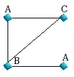
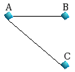
 |

|
| Graph 1 |
Graph 2 |
For Graph1, we have the following shortest paths
of length 1 up to LP=3.
starting from the upper node A :
{A,AC,AB,ABA}
starting from the node B : {B,BC,BA,BA}
starting from the
downer node A : {A,AB,ABC,ABA}
starting from the node C :
{C,CA,CB,CBA}
For Graph2, we have the following shortest paths of length
1 up to LP=3.
starting from the node A : {A,AB,AC}
starting from the node
B : {B,BA,BAC}
starting from the node C : {C,CA,CAB}
When edges are
undirected, the path XYZ is equal to path ZYX, and we form the following matrix A:
| A= |
| Graph |
C |
CA |
CB |
CBA |
A |
AB |
ABA |
B |
BAC |
| Graph1 |
1 |
2 |
2 |
2 |
2 |
4 |
2 |
1 |
0 |
| Graph2 |
1 |
2 |
0 |
0 |
1 |
2 |
0 |
1 |
2 |
|
Once the matrix A is
created both algorithms take all rows and cluster them using distances - either
inner product or Euclidean distance (Euclidean in this example), chosen by the
user.
To use any algorithm of GraphClust you have to: (1) create a dataset
file; (2) choose your options.
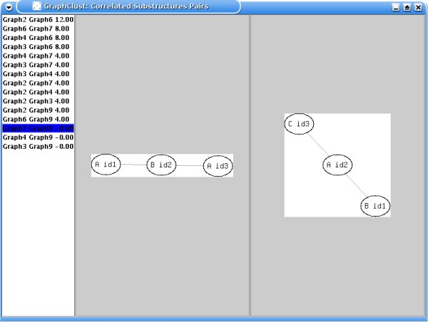
In addition, correlated (i.e. highly
co-occurring) substructures pairs are displayed in descending order of
correlation, as shown in the following example:

For each substructure, the nodes, painted as circles, have a label
and an identification number. A circle containing the dot symbol is used as a
dummy which means that the proposed substructure has only 1 node (the one linked
to the circle with the dot symbol). Two input parameters are here involved:
- -min m. Only substructures having at least m nodes are
shown.
Options: integer value.
Default: 1.
- -SVD r. By using SVD, the substructure-graph matrix
AT is broken apart into the product of 3 matrices T,
S and DT based on the singular value
decomposition (SVD). These matrices are truncated to r dimensions. Dimensionality reduction reduces "noise" in the substructure-substructure matrix showing a richer
relationship between the substructures.
Finally, the substructure-substructure
correlation matrix X is computed multiplying Tr×Sr×(Tr
×Sr)T and its values are displayed.
Options:
integer value.
Default: number of input graphs.
Let us consider the substructure-graph matrix AT of the two graphs Graph1 and Graph2 showed above:
| AT= |
| Substructures |
Graph1 |
Graph2 |
| C |
1 |
1 |
| CA |
2 |
2 |
| CB |
2 |
0 |
| CBA |
2 |
0 |
| A |
2 |
1 |
| AB |
4 |
2 |
| ABA |
2 |
0 |
| B |
1 |
1 |
| BAC |
0 |
2 |
|
The Singular Value Decomposition of AT creates the following matrices T,
S, DT.
| AT= |
| -0.20 |
-0.17 |
| -0.40 |
-0.33 |
| -0.26 |
0.35 |
| -0.26 |
0.35 |
| -0.33 |
0.01 |
| -0.66 |
0.02 |
| -0.26 |
0.35 |
| -0.20 |
-0.17 |
| -0.13 |
-0.68 |
|
× |
|
× |
|
|
T |
× |
S |
× |
DT |
Let us suppose the parameter r=1. The reduced matrices are Tr,
Sr, DTr.
Then, the reduced correlation substructure-substructure matrix Xr is equal to Tr×Sr×(Tr
×Sr)T
| Xr= |
| -0.20 |
| -0.40 |
| -0.26 |
| -0.26 |
| -0.33 |
| -0.66 |
| -0.26 |
| -0.20 |
| -0.13 |
|
× |
|
× ( |
| -0.20 |
| -0.40 |
| -0.26 |
| -0.26 |
| -0.33 |
| -0.66 |
| -0.26 |
| -0.20 |
| -0.13 |
|
×
|
|
)T= |
|
C |
CA |
CB |
CBA |
A |
AB |
ABA |
B |
BAC |
| C |
2 |
4 |
2 |
2 |
3 |
6 |
2 |
2 |
2 |
| CA |
4 |
8 |
4 |
4 |
6 |
12 |
4 |
4 |
4 |
| CB |
2 |
4 |
4 |
4 |
4 |
8 |
4 |
2 |
0 |
| CBA |
2 |
4 |
4 |
4 |
4 |
8 |
4 |
2 |
0 |
| A |
3 |
6 |
4 |
4 |
5 |
10 |
4 |
3 |
2 |
| AB |
6 |
12 |
8 |
8 |
10 |
20 |
8 |
6 |
4 |
| ABA |
2 |
4 |
4 |
4 |
4 |
8 |
4 |
2 |
0 |
| B |
2 |
4 |
2 |
2 |
3 |
6 |
2 |
2 |
2 |
| BAC |
2 |
4 |
0 |
0 |
2 |
4 |
0 |
2 |
4 |
|
| Tr | × |
Sr |
× ( | Tr |
× | Sr | )T |
The output of "graphclust"
includes a file named 'output' and a directory named 'correlation_files'.
The first one displays all the generated clusters and for each cluster it
displays the centroid, all its elements and the distances of each element from
the centroid.
The second one contains all the information pertaining to
correlated substructures.
There are many applications for graph clustering. Some requests we have
received have to do with Internet search engines, knowledge management systems,
document databases and XML document management.
Home
GraphClust is implemented in ANSI C, the graphical interface is implemented
in JAVA and the substructure images are built by using the springgraph
command.
Home
To download GraphClust, please send email to shasha@cs.nyu.edu and to diegoref@dmi.unict.it.
If you care to
describe your application, we'd be glad to hear about it. In any case, we will
send you instructions for downloading the program.
Home
GraphClust is implemented
in ANSI C. It has been
ported on Unix, and Windows platforms.
To install
GraphClust:
- Unzip the GraphClust package
- type "cd GraphClust"
- type "cd src"
- type "make"
- type "cd .."
- Check if there is "graphclust_main", "graphclustA", "graphclustA_S",
"graphclustB", "graphclustB_S" existing in the current folder
- Download the SubDue5.1 release from the download section at http://ailab.uta.edu/subdue/
- unzip the zip file where you want
- go to subdue-5.1.0/src directory
- type make
- copy binary files sgiso and subdue to the directory that graphclust_main,
graphclustA, graphclustA_S and graphclustB_S are in.
- type ./graphclust_main without arguments to see all the possible options.
- Check if the springgraph command is present in own unix system. (Even
without it, the sotware still works but it will not show the substructures
images).
For bugs and questions please contact diegoref@dmi.unict.it or shasha@cs.nyu.edu.
Home
Usage of
GraphClust
File
formats
- dataset file
The file consists of a collection of graph
specifications (LNE=List of Nodes and Edges ids format). The first
line of each graph must begin with the character '#' and contains the
label of the graph; it can be a number or a string. The next line contains the
number of nodes in the graph. Subsequent lines contain the nodes'
labels, one label per line. The first label is the label of node 0, the next
one is the label of node 1, etc. Next is the number of edges in the
graph, followed by a list of edges consisting of node id pairs. Each line
contains only one edge. An example of dataset file is given in here.
- output
file
The output is given in a file called "output". Each
Cluster is identified by an index number (starting from 1) with the number of
graphs in the cluster and the radius in square brackets. In the next row we
have the centroid of the cluster. In the subsequent rows we have the other
elements, if any, and their distance from the centroid in brackets.
(see
example here ).
The "correlation_files" directory includes all the information
already showed in the form.
Running
GraphClust
To run the examples go to the GraphClust directory and do the
following
- Execution
type
graphclust_main dataset_file_name".
You have to specify if you want to run the kmeans algorithm with the option
-kmeans k where k is the number of clusters you want or with the
Antipole algorithm with the option -tightness measure where
measure is 1..4.
Other options are:
- -s S in order to use subdue algorithm to find the substructures
- -s P in order to use shortest path to find the substructures
- -g D to deal with directed graphs
- -g U to deal with undirected graphs
- -m I to use the inner product metric
- -m E to use the Euclidean distance
- -min m to show the substructures whose number of nodes is greater
or equal than m
- -SVD r to reduce the substructure-substructure correlation matrix
by using the SVD algorithm retaining the most r meaningful rows.
Home
Clustering References


