Evaluation of DB2 Query Optimizer and SQL99 Implementation

Pareena Parikh

Independent Study, Summer 2002

New York University, Department of Computer Science

Advisors: Alberto Lerner, Dennis Shasha

8/9/2002

Abstract

The SQL 99 Standard introduces much-needed analytical capabilities to relational database querying, resulting in increased ability to perform dynamic, analytic SQL queries. While the new constructs provide syntax for more complex calculations, this study focuses on evaluating the ability of the Relational Database query optimizer to create efficient access plans for returning results. Particularly, in this study, we evaluate (i) DB2’s implementation of the SQL 99 Standard in terms of query readability and development, and (ii) DB2’s query optimizer for generating access plans – using a test set of irregular and regular time series financial data, and a benchmark set of analyses. First, our results show that, while the DB2 implementation provides sufficient syntax for most queries considered, it does leaves some room for improvement from a query readability and development standpoint. While we are able to find “work-arounds” to achieve complex calculations, some examples of deficiencies we noted include the lack of FIRST/LAST aggregate functions and lack of PRODUCT aggregate function. Second, we find that, for the cases considered, the DB2 Optimizer performs well in terms of optimizing aggregations that use the OVER clause, and performs average in terms of general SORT Order Management. Some examples of deficiencies noted are extraneous sorts or sorts that occur later in the access plan than necessary. Some examples of efficiencies noted are consolidation of SORTS so that they handle multiple aggregations on the same OVER partition, propagation of SORT results from one partition to a superset partition (i.e., for example, the sort on week(tradedate) to month(tradedate) to year(tradedate) – each result is propagated to the next instead of performing each one independently).

Table of Contents

1. Introduction

2. Objective

3. Background

3.1. SQL99

4. Query Optimization

4.1. Cost Based Optimization

4.2. Logical Plan Optimization

4.3. Physical Plan Optimization

5. Experimental Design

5.1. Tick Database

5.1.1. Data Model

5.2. Markets Database

5.2.1. Data Model

6. Experimental Setup

7. Test Results Detail

7.1. Ticks

7.1.1. Query Spec

7.1.2. Syntax and Access Plans

7.1.3. Detailed Analysis

7.2. Markets

7.2.1. Query Spec

7.2.2. Syntax and Access Plans

7.2.3. Detailed Analysis

8. Test Results Summary

8.1. Query Readability

8.2. Query Optimization

9. Analysis and Conclusions

9.1. Query Readability

9.2. Plan Optimization

References

Introduction

Relational databases form the foundation of many systems, both in industry and in academics, ranging in application from ERP systems to data warehouses to e-commerce platforms. The power of databases comes from a body of knowledge and technology that has developed over several decades. Some types of databases are: hierarchical, network, inverted list, and relational. Most applications rely on relational databases, which are commonly available in the form of Relational Database Management Systems (RDBMS).

Among other features, an RDBMS provides users with persistent storage, a programming interface, and transaction management [1] . RDBMS’ generally have many different components – including a transaction manager, query compiler, execution engine, logging and recovery modules, concurrency control modules, and storage managers [2]. For the purposes of this study, we will focus on the query compiler, which is the one component that affects data retrieval performance most. The query compiler contains 3 parts:

1) query parser

2) query preprocessor

3) query optimizer

We will measure the performance of the query optimizer, which transforms the initial query plan – generated by the query preprocessor – into the best available sequence of operations on the actual data, in this study.

IBM initially introduced DB2 version 1.0 as its RDBMS in 1984. Since then, it has seen many versions and has gained credibility as one of the major RDBMS products in industry.

Objective

The purpose of this study is to evaluate DB2’s capability to optimize SQL statements, with a particular emphasis on the SQL 99 standard OLAP functions. This qualitative analysis will rate DB2 in the areas of access plan generation and query readability, and provide a foundation for detailed performance benchmarks.

In the next two sections we are going to introduce the OLAP extensions of SQL:1999 and give an overview of the internal workings of an optimizer that compiles such queries The reader familiar with these topics could skip to section 5, Experimental Design.

Background

SQL 99 Standard for Analytics

With the advent of SQL 99, the SQL language has advanced data partitioning and ordering capabilities, which lends well to analysis. Particularly, the OLAP Functions provide aggregation and windowing constructs. Database vendors implement and, in some cases, extend the standard in slightly different ways. As we are evaluating DB2, we will review its implementation here. DB2 provides the following OLAP specification [3]:

OLAP-function
 |--+-| ranking-function |-----+---------------------------------|
 +-| numbering-function |---+
 '-| aggregation-function |-'
 
ranking-function
 |---+-RANK ()-------+--OVER------------------------------------->
 '-DENSE_RANK ()-'
 
>----(--+------------------------------+------------------------>
 '-| window-partition-clause |--'
 
>----| window-order-clause |--)---------------------------------|
 
numbering-function
 |---ROW_NUMBER ()--OVER---(--+------------------------------+--->
  '-| window-partition-clause |--'
 
>----+--------------------------+---)---------------------------|
 '-| window-order-clause |--'
 
aggregation-function
 |---column-function--OVER---(--+------------------------------+->
  '-| window-partition-clause |--'
 
>----+--------------------------+------------------------------->
 '-| window-order-clause |--'
 
 .-RANGE BETWEEN UNBOUNDED PRECEDING AND UNBOUNDED FOLLOWING--.
>----+------------------------------------------------------------+---)->
 '-| window-aggregation-group-clause |------------------------'
 
>---------------------------------------------------------------|
 
window-partition-clause
 .-,--------------------------.
 V |
|---PARTITION BY-----partitioning-expression---+----------------|
 
window-order-clause
 .-,-------------------------------.
 V .-ASC--. |
|---ORDER BY-----sort-key-expression--+------+--+---------------|
 '-DESC-'
 
window-aggregation-group-clause
|---+-ROWS--+---+-| group-start |---+---------------------------|
 '-RANGE-' '-| group-between |-'
 
group-start
|---+-UNBOUNDED PRECEDING-----------+---------------------------|
 +-unsigned-constant--PRECEDING--+
 '-CURRENT ROW-------------------'
 
group-between
|---BETWEEN--| group-bound1 |--AND--| group-bound2 |------------|
 
group-bound1
|---+-UNBOUNDED PRECEDING-----------+---------------------------|
 +-unsigned-constant--PRECEDING--+
 +-unsigned-constant--FOLLOWING--+
 '-CURRENT ROW-------------------'
 
group-bound2
|---+-UNBOUNDED FOLLOWING-----------+---------------------------|
 +-unsigned-constant--PRECEDING--+
 +-unsigned-constant--FOLLOWING--+
 '-CURRENT ROW-------------------'
 

On-Line Analytical Processing (OLAP) functions provide the ability to return ranking, row numbering and existing column function information as a scalar value in a query result. An OLAP function can be included in expressions in a select-list or the ORDER BY clause of a select-statement (SQLSTATE 42903). An OLAP function cannot be used as an argument of a column function (SQLSTATE 42607). The query result to which the OLAP function is applied is the result table of the innermost subselect that includes the OLAP function.

When specifying an OLAP function, a window is specified that defines the rows over which the function is applied, and in what order. When used with a column function, the applicable rows can be further refined, relative to the current row, as either a range or a number of rows preceding and following the current row. For example, within a partition by month, an average can be calculated over the previous three month period.

The ranking functions, RANK and DENSE_RANK, compute the ordinal rank of a row within the window. Rows that are not distinct with respect to the ordering within their window are assigned the same rank. The results of ranking may be defined with or without gaps in the numbers resulting from duplicate values.

The ROW_NUMBER ³⁷ function computes the sequential row number of the row within the window defined by the ordering, starting with 1 for the first row. If the ORDER BY clause is not specified in the window, the row numbers are assigned to the rows in arbitrary order as returned by the subselect (not according to any ORDER BY clause in the select-statement).

In addition, SQL 99 introduces the WITH clause for use with the SELECT statement, allowing for more flexible sub-querying and a more intuitive syntactic representation of subqueries as “local” views. One of the main benefits of this DB2 provides the following WITH clause implementation [4]:

SELECT STATEMENT

>>-+-----------------------------------+--fullselect------------>
 | .-,-----------------------. |
 | V | |
 '-WITH----common-table-expression-+-'
 
>--+-----------------+--+--------------------+------------------>
 '-order-by-clause-' '-fetch-first-clause-'
 
 .----------------------.
 V | (1) (2)
>----+------------------+-+------------------------------------><
 +-update-clause----+
 +-read-only-clause-+
 +-optimize-clause--+
 '-isolation-clause-'
 
 

Notes:

1. The update-clause and read-only-clause cannot both be specified in the
same select-statement.

2. Each clause may be specified only once.

The select-statement is the form of a query that can be directly specified in a DECLARE CURSOR statement, or prepared and then referenced in a DECLARE CURSOR statement. It can also be issued interactively, using the interactive facility (STRSQL command), causing a result table to be displayed at your work station. In either case, the table specified by a select-statement is the result of the fullselect.

COMMON TABLE EXPRESSION

>>-table-name--+-----------------------+--AS--(--subselect--)--><
 | .-,-----------. |
 | V | |

'-(----column-name-+--)-'

A common-table-expression permits defining a result table with a table-name that can be specified as a table name in any FROM clause of the fullselect that follows. The table-name must be unqualified. Multiple common table expressions can be specified following the single WITH keyword. Each common table expression specified can also be referenced by name in the FROM clause of subsequent common table expressions.

If a list of columns is specified, it must consist of as many names as there are columns in the result table of the subselect. Each column-name must be unique and unqualified. If these column names are not specified, the names are derived from the select list of the subselect used to define the common table expression.

The table-name of a common table expression must be different from any other common table expression table-name in the same statement. A common table expression table-name can be specified as a table name in any FROM clause throughout the fullselect. A table-name of a common table expression overrides any existing table, view, or alias (in the catalog) with the same qualified name.

If more than one common table expression is defined in the same statement, cyclic references between the common table expressions are not permitted. A cyclic reference occurs when two common table expressions dt1 and dt2 are created such that dt1 refers to dt2 and dt2 refers to dt1.

A common-table-expression is also optional prior to the subselect in the CREATE VIEW and INSERT statements.

A common-table-expression can be used:

· In place of a view to avoid creating the view (when general use of the view is not required and positioned updates or deletes are not used

· When the desired result table is based on host variables

· When the same result table needs to be shared in a fullselect

If a subselect of a common table expression contains a reference to itself in a FROM clause, the common table expression is a recursive table expression.

Query Optimizer

The Query Optimizer of a relational database consists of two parts: (i) the logical plan generation, during which the query parse tree is converted into an initial query plan, which is then transformed into an equivalent logical plan that is expected to require less time to execute, and (ii) physical plan generation, where the abstract query plan is turned into a physical query plan by selecting algorithms to implement each operator in the logical query plan, and an order of execution for these operators [5].

Cost Based Optimization

We assume that cost of evaluating an expression is approximated by the number of disk I/Os performed. The number of disk I/Os is influenced by [7]:

· The particular logical operators chosen to implement the query.

· The size of intermediate relations.

· The physical operators used to implement the logical operators.

· The ordering of similar operations.

· The method of passing arguments from one physical operator to the next.

Logical Plan Optimization

Pushing Down Selections

Selections are crucial operations because they reduce the size of relations significantly. One of the most important rules of efficient query processing is to move selections down the tree as far as they will go without changing what the expression does [6]. If a selection condition is the AND of several conditions, then we can split the condition and push each piece down the tree separately.

Choosing Join Order

Selecting the join order for the join of three or more relations is a critical problem in query optimization. The one-pass join reads one relation (preferably the smaller) into main memory, creating a hash table to facilitate matching of tuples from the other relation. It then reads the other relation, one block at a time, to join its tuples with the tuples stored in memory. In this case, the left argument of the join is the smaller relation that is to be stored in main memory while the right argument of a join is read a block at a time and matched to the stored relation. Other join algorithms include: nested loop joins, and index joins [10].

Heuristics for Reducing the Cost of the Logical Query Plan

There are many heuristics for reducing the cost of the logical query plan. By estimating the cost both before and after a transformation, the optimizer decides to keep the transformation where it appears to reduce cost, and avoid the transformation otherwise [9].

Physical Plan Optimization

Choosing Selection Method

In the physical plan optimization step, the optimizer must estimate the lowest cost selection operation. An outline of how costs are estimated is as follows [11]:

1) The cost of Table Scan coupled with Filter, a) if relation is clustered, or b) if relation is not clustered.

2) The cost of an algorithm that picks an equality term such as a=10 for which an index on attribute a exists uses Index Scan to find the matching tuples, and then filters the retrieved tuples to see if they match the full condition, a) if the index is clustering, b) if the index is non-clustering

3) The cost of an algorithm that picks an inequality term such as b<20 for which an index on attribute b exists uses Index Scan to find the matching tuples, and then filters the retrieved tuples to see if they match the full condition, a) if the index is clustering, b) if the index is non-clustering.

Choosing Join Method

Several options exist when choosing the join method. Some approaches are [12]:

1) One pass join – this approach assumes that the buffer manager can devote enough buffers to the join, or that the buffer manager can come close so that thrashing is not a major problem. An alternative is the Nested Loop join.

2) Sort Join

3) Index Join

4) Multipass Join using hashing

Materialization versus Pipelining

The approach where each intermediate relation in a query plan is stored on disk for the next operation in sequence to access is termed “materialization”. A more subtle and generally more efficient way to execute a query plan is to have several operations running at once. The tuples produced by one operation are passed directly to the operation that uses it, without ever storing the intermediate tuples on disk. This approach is called “pipelining”.

Experimental Design

The test database, including data model and generated data, was based on the FinTime Specification, a financial time series benchmark, authored by Dennis Shasha and available at www.cs.nyu.edu/cs/faculty/shasha/fintime.d/bench.html. The specification consists of two databases: Ticks and Markets.

Tick Database

Ticks are price quotations of trade prices and associated attributes for individual securities that occur either on the floor of a stock exchange or in an electronic trading system. Ticks include two basic types of data: 1) trades that are transactions between buyers and sellers at a fixed price and quantity, and 2) Quotes that are the price quotations offered by buyers and sellers.

Data Model

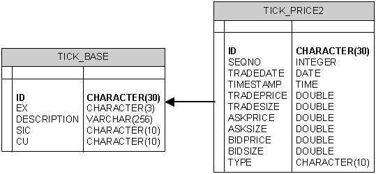
The data model is as follows, with TICK_BASE having a 1:Many relation with TICK_PRICE2 on ID:

Markets Database

Market information is provided as a set of files by a market data vendor, available at the end of each trading day. Thus, the market data contains an entry for each security for each trading day, a regular time series. Along with this data, we have dividends and splits, each of which are irregular time series, representing events that affect the price and volume of particular securities.

Data Model

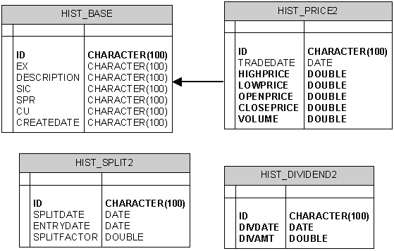
The data model is as follows, with HIST_BASE having a 1:Many relation with HIST_PRICE2, HIST_SPLIT2, and HIST_DIVIDEND2:

Experimental Setup

Data for all tables except Splits and Dividends was generated into comma delimited flat files using a C++ program designed for the FinTime benchmark.

Splits and Dividend data was generated manually (by running an insert statement for each row). For the Ticks Database, we generated ticks for 5 securities with ~5500 ticks per day for 10 days, resulting in 284000 rows in the TICK_PRICE2 table. For the Markets Database, we generated data for 500 securities for 30 days (and by definition, there is one record per day), resulting in 15000 rows in the HIST_PRICE2 table. For Splits, we generated splits for 10 securities, some of which had multiple splits. For Dividends, we generated 3 dividends for 5 securities, resulting in 15 rows in the HIST_DIVIDEND2 table.

Schema Generation and Data Loading for most tables were done via the DB2 Control Center. Splits and Dividends were loaded using Insert statements.

Test Results Detail

The testing was done incrementally for each query. By adding database optimizations or rearranging clauses/syntax in each phase, we attempt to show how the optimizer performs under different circumstances. In this section, we show the details of each query that was executed, and its access plans. The following section evaluates the DB2 optimizer and readability with respect to each query.

Ticks Database

Query 1

Specification:

1	Get all ticks for a specified set of 100 securities for a specified three hour time period on a specified trade date.

Syntax and Access Plans:

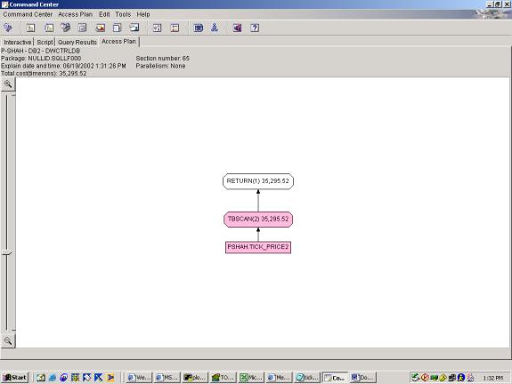
Two attempts were made at this simple query. The syntax is the same in each attempt, but in the first case, we have no indexes, and in the second case, we have an index on ID and an index on TRADEDATE, TIMESTAMP.

--Q1.1 SELECT TICKS (NO INDEXES)

SELECT *

FROM tick_price2

WHERE tradedate = '06/13/2002'

AND timestamp BETWEEN '09:00:00' AND '12:00:00'

AND id LIKE 'id_5%'

--Q1.2 SELECT TICKS (WITH INDEXES)

SELECT *

FROM tick_price2

WHERE tradedate = '06/13/2002'

AND timestamp BETWEEN '09:00:00' AND '12:00:00'

AND id LIKE 'id_5%'

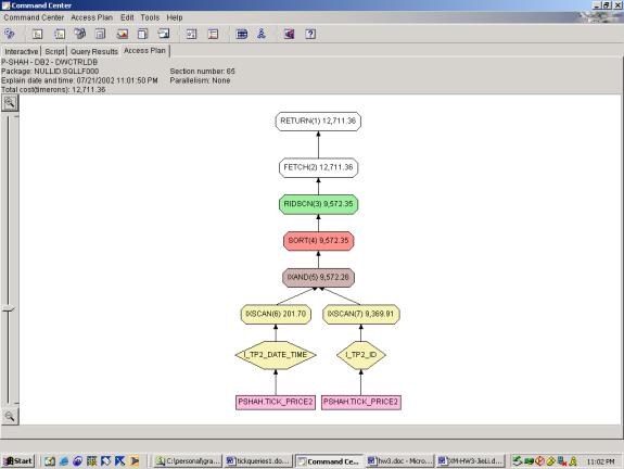
Detailed Analysis: This query was a simple selection with 3 predicates. The criteria were changed slightly to accommodate the generated data, but shouldn’t affect the overall plan. The first query attempt shows a basic access plan. The second query attempt shows use of both indexes, with an INDEX AND to merge the results, and interestingly, the optimizer chooses to SORT the result of the INDEX AND on ROWID prior to looking up rows. This is very smart because it saves multiple lookups to the same page (which would be the case if it was not sorted on ROWID).

Query 2

Specification:

2.	Determine the volume weighted price of a security considering only the ticks in a specified three hour interval

Syntax and Access Plans:

Two attempts were made at this query. The syntax is the same in each attempt, but in the first case, we have no indexes, and in the second case, we have an index on ID and an index on TRADEDATE, TIMESTAMP.

--Q2.1 VOLUME WEIGHTED PRICE (NO INDEXES)

SELECT id,

sum(tradesize*tradeprice)/sum(tradesize)

FROM tick_price2

WHERE tradedate = '06/13/2002'

AND timestamp BETWEEN '09:00:00' AND '12:00:00'

AND id LIKE 'Security%'

GROUP BY id

--Q2.2 VOLUME WEIGHTED PRICE ( INDEXES )

SELECT id,

sum(tradesize*tradeprice)/sum(tradesize)

FROM tick_price2

WHERE tradedate = '06/13/2002'

AND timestamp BETWEEN '09:00:00' AND '12:00:00'

AND id LIKE 'Security%'

GROUP BY id

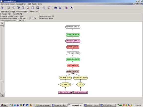
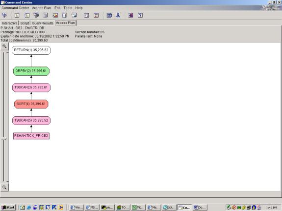
Detailed Analysis: This query was a selection with 3 predicates and 1 aggregation. The criteria were changed slightly to accommodate the generated data, but shouldn’t affect the overall plan. The first query attempt shows a basic access plan with the <SORT, TABLESCAN, GROUPBY> pattern to accomplish the aggregation. The TABLESCAN in this pattern is a low-cost scan of the temporary table that the SORT result was stored into (this is done presumably to provide for the case where the SORT result is too large to fit in memory). The second query attempt shows the same, however it uses both indexes, with an INDEX AND to merge the results, and interestingly, the optimizer chooses to SORT the result of the INDEX AND on ROWID prior to looking up rows. This is very smart because it saves multiple lookups to the same page (which would be the case if it was not sorted on ROWID).

Query 3

Specification:

3.	Determine the top 10 percentage losers for the specified date on the specified exchanges sorted by percentage loss. The loss is calculated as a percentage of the last trade price of the previous day.

Syntax and Access Plans:

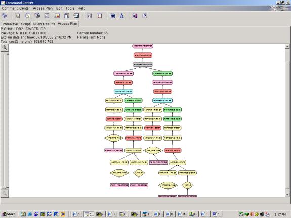
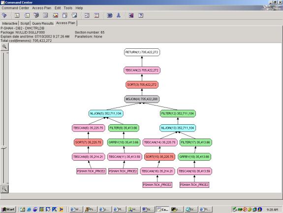
Nine attempts were made on this query. Q3.9 shows the worst case scenario, where we have 2 subqueries, with 1 subquery each, that each require a full table scan on the original table, TICK_PRICE2. The structure is as follows:

The results of the each pair – the subquery and sub-sub-query -- are joined using a very costly nested loop join, and then the results of the 2 nested loop joins are joined in a merge join. Q3.8 shows the same query syntax, but improves the situation (reducing cost to 1/5 of Q3.9) by adding two indexes, one on ID and the other on TRADEDATE, TIMESTAMP. 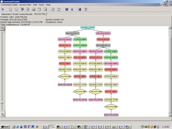The plan is very similar in the sequence of operations, except that it uses index scans instead of full tablescans. Q3.7 is a query rewrite that changes the nesting so that there are essentially 4 subqueries and 0 sub-sub-queries. Thus, the 2 costly nested loop joins are removed and instead we merge join 2 subqueries, the results of which are then joined in a nested loop join:

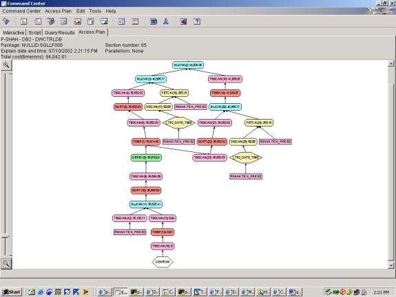
This restructuring of the query, and reversal of the join types in the access plan significantly improves performance (by 30%). Q3.6 query rewrite further improves the situation by reducing from 4 to 3 subqueries (and more importantly from 4 to 3 full tablescans on TICK_PRICE2). Realizing that we can get yesterday’s and today’s max timestamp for each id in one query, we are able to reduce the cost. Interestingly, we access the twodays subquery twice in the main SELECT clause, but it doesn’t add much to the cost since the twodays table is so small (in comparison to TICK_PRICE2). 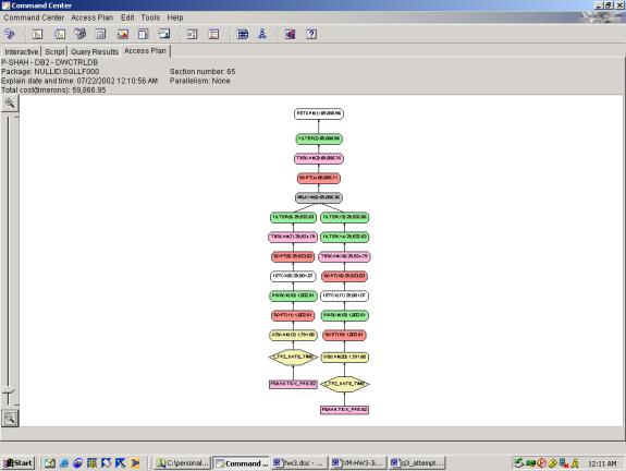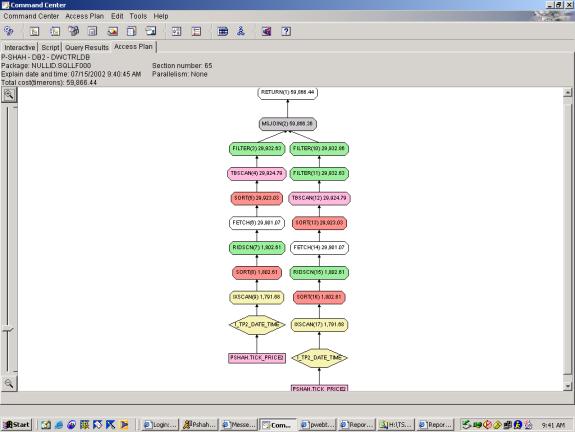Q3.5 query rewrite cuts cost nearly in half by adding an OVER clause in order to obtain max timestamp in the same query as the rest of the information, bumping down from 3 to 2 full tablescans. The results of the 2 subqueries are then joined in a merge join. Q3.4 adds the extra top ten filter (which up until now was assumed to be done at the client), with little extra cost. The plan is exactly the same as Q3.5 with the exception of the aggregation at the end. 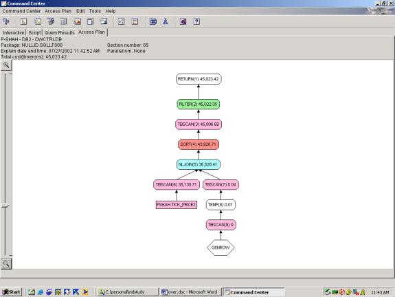This <sort, aggregation and filter> is low cost presumably since the data set is so small at this point. Q3.3 shows yet another milestone, reducing down from 2 full tablescans to 1 full tablescan by adding a tricky OVER clause to get previous day price and current day price in the same row. In this case, the WITH clause was key because it allows us to build one query off of another query without rewriting it as a subquery. We reduce cost by another 25% in this pass. 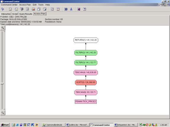With one tablescan on the original table, there is essentially no join operation (the nested loop join that appears is very low cost because it joins a single row with the result of the single tablescan) and the single sort takes care of both the sort on the original table and the sort which gets us the previous price. Q3.2 tests how well the optimizer performs in pushing down filters. It is similar to Q3.3, however it moves the filters into the main SELECT clause instead of in the 2 subqueries. The results show that the optimizer does not push down the filters, thus the sort is much more costly (due to a larger data set), and the cost shoots up to 3 times that in Q3.3).

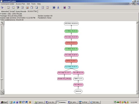
The final pass, Q3.1, is the most efficient plan and retrieves results that are closest to the specification. It is essentially a rewrite of Q3.3 with the only difference being that it performs the top ten filter. Interestingly, the cost is only slightly larger than without the top ten filter. This may be due to the fact that the data set is so small by the time it gets to the ranking, and thus the sort on rank is low-cost.

--Q3.1 TOP 10 PERCENTAGE LOSERS (1 TABLE SCAN ON TICK_PRICE2, USES OVER, TOP TEN FILTER INCLUDED)

Adding top ten:

WITH

LAStTs (id, tradedate, tradeprice, lASttime) AS

(SELECT id,

tradedate,

tradeprice,

ROW_NUMBER() OVER (PARTITION BY id, tradedate ORDER BY timestamp DESC) AS rown

FROM Tick_price2

WHERE tradedate='6/21/2002' or tradedate='6/20/2002'),

CurrTs (id, tradedate, tradeprice, prevprice) AS

(SELECT id,

tradedate,

tradeprice,

avg(tradeprice) OVER (PARTITION BY id ORDER BY tradedate ASc ROWS BETWEEN 2 preceding AND 1 preceding)

FROM LAStTs

WHERE lASttime=1),

result (id, percLoss,percLossRank) AS

(SELECT id,

(prevprice-tradeprice)*100/prevprice perc_loss, rank() OVER (ORDER BY (prevprice-tradeprice)*100/prevprice)

FROM CurrTs

WHERE tradedate='6/21/2002')

SELECT *

FROM result

WHERE percLossRank<4

--Q3.2 TOP 10 PERCENTAGE LOSERS (1 TABLE SCAN ON TICK_PRICE2, USES OVER, CLIENT SIDE TOP TEN FILTER & SORT, ATTEMPT TO MAKE OPTIMIZER PUSH DOWN FILTERS)

WITH

LAStTs (id, tradedate, tradeprice, lASttime) AS

(SELECT id,

tradedate,

tradeprice,

ROW_NUMBER() OVER (PARTITION BY id, tradedate ORDER BY timestamp DESC) AS rown

FROM Tick_price2),

CurrTs (id, tradedate, tradeprice, prevprice) AS

(SELECT id,

tradedate,

tradeprice,

avg(tradeprice) OVER (PARTITION BY id ORDER BY tradedate ASc ROWS BETWEEN 2 preceding AND 1 preceding) FROM LAStTs

WHERE lASttime=1)

SELECT id,

tradedate,

tradeprice,

prevprice,

(prevprice-tradeprice)*100/prevprice perc_loss

FROM

CurrTs

WHERE tradedate='6/20/2002' or tradedate='6/19/2002'

Total cost=141142.20

--Q3.3 TOP 10 PERCENTAGE LOSERS (1 TABLE SCAN ON TICK_PRICE2, USES OVER, CLIENT SIDE TOP TEN FILTER & SORT)

WITH

LAStTs (id, tradedate, tradeprice, lASttime) AS

(SELECT id,

tradedate,

tradeprice,

ROW_NUMBER() OVER (PARTITION BY id, tradedate ORDER BY timestamp DESC) AS rown

FROM Tick_price2

WHERE tradedate='6/20/2002' or tradedate='6/19/2002'),

CurrTs (id, tradedate, tradeprice, prevprice) AS

(SELECT id,

tradedate,

tradeprice,

avg(tradeprice) OVER (PARTITION BY id ORDER BY tradedate ASc ROWS BETWEEN 2 preceding AND 1 preceding)

FROM LAStTs

WHERE lASttime=1)

SELECT id,

tradedate,

tradeprice,

prevprice,

(prevprice-tradeprice)*100/prevprice perc_loss

FROM

CurrTs

Total cost=45023.42

--Q3.4 TOP 10 PERCENTAGE LOSERS (2 TABLE SCANS ON TICK_PRICE2, USES OVER, TOP TEN FILTER INCLUDED)

WITH

LAStTs (id, tradedate, tradeprice, lASttime) AS

(SELECT id,

tradedate,

tradeprice,

ROW_NUMBER() OVER (PARTITION BY id, tradedate ORDER BY timestamp DESC) AS rown

FROM Tick_price2

WHERE tradedate='6/12/2002'),

CurrTs (id, tradedate, tradeprice, lASttime) AS

(SELECT id,

tradedate,

tradeprice,

ROW_NUMBER() OVER (PARTITION BY id, tradedate ORDER BY timestamp DESC) rown

FROM Tick_price2

WHERE tradedate='6/13/2002'),

allids (id, rank) AS

(SELECT a.id,

rank() OVER (ORDER BY a.tradeprice*100/b.tradeprice DESC)

FROM

LAStTs a, CurrTs b

WHERE

a.id=b.id

AND a.lASttime=1

AND b.lASttime=1)

SELECT id

FROM allids

WHERE rank<11

--Q3.5 TOP 10 PERCENTAGE LOSERS (2 TABLE SCAN ON TICK_PRICE2, USES OVER, CLIENT SIDE TOP TEN FILTER AND SORT)

WITH

LAStTs (id, tradedate, tradeprice, lASttime) AS

(SELECT id,

tradedate,

tradeprice,

ROW_NUMBER() OVER (PARTITION BY id, tradedate ORDER BY timestamp DESC) AS rown

FROM Tick_price2

WHERE tradedate='6/12/2002'),

CurrTs (id, tradedate, tradeprice, lASttime) AS

(SELECT id,

tradedate,

tradeprice,

ROW_NUMBER() OVER (PARTITION BY id, tradedate ORDER BY timestamp DESC) rown

FROM Tick_price2

WHERE tradedate='6/13/2002')

SELECT a.id,

a.tradeprice*100/b.tradeprice

FROM LAStTs a, CurrTs b

WHERE a.id=b.id

AND a.lASttime=1

AND b.lASttime=1

total cost= 59M

--Q3.6 TOP 10 PERCENTAGE LOSERS (3 TABLE SCANS ON TICK_PRICE2, CLIENT SIDE TOP TEN FILTER AND SORT)

WITH

twodays

(id,tradedate,timestamp) AS (SELECT id, tradedate,max(timestamp)

FROM tick_price2

WHERE tradedate='6/12/2002' or tradedate='6/13/2002'

GROUP BY id, tradedate )

SELECT b.tradeprice*100/a.tradeprice,

b.id

FROM

tick_price2 a,

tick_price2 b,

twodays c,

twodays d

WHERE a.timestamp=c.timestamp

AND a.id=c.id

AND a.tradedate='6/12/2002'

AND c.tradedate='6/12/2002'

AND b.timestamp=d.timestamp

AND b.id=d.id

AND b.tradedate='6/13/2002'

AND d.tradedate='6/13/2002'

--Q3.7 TOP 10 PERCENTAGE LOSERS (3 JOIN, CLIENT SIDE TOP TEN FILTER AND SORT)

WITH

yesterday

(id,timestamp) AS (SELECT id, max(timestamp) FROM tick_price2 WHERE tradedate='6/12/2002' GROUP BY id),

today (id, timestamp) AS (SELECT id, max(timestamp) FROM tick_price2 WHERE tradedate='6/13/2002' GROUP BY id)

SELECT b.tradeprice*100/a.tradeprice,

b.id

FROM

tick_price2 a,

tick_price2 b,

today,

yesterday

WHERE a.timestamp=yesterday.timestamp

AND a.id=yesterday.id

AND a.tradedate='6/12/2002'

AND b.timestamp=today.timestamp

AND b.id=today.id

AND b.tradedate='6/13/2002'

--Q3.8 TOP 10 PERCENTAGE LOSERS (3 JOIN, CLIENT SIDE TOP TEN FILTER)

SELECT (z.tradeprice*100)/y.tradeprice, z.id

FROM

(SELECT tradeprice,id

FROM tick_price2 x

WHERE timestamp=(SELECT max(timestamp) FROM tick_price2 WHERE id=x.id AND tradedate='06/12/2002')

AND tradedate='06/12/2002') y,

(SELECT tradeprice,id

FROM tick_price2 w

WHERE timestamp=(SELECT max(timestamp) FROM tick_price2 WHERE id=w.id AND tradedate='06/13/2002')

AND tradedate='06/13/2002') z

WHERE y.id=z.id

ORDER BY (z.tradeprice*100)/y.tradeprice DESC

--Q3.9 TOP 10 PERCENTAGE LOSERS (3 JOIN, CLIENT SIDE TOP TEN FILTER)

SELECT (z.tradeprice*100)/y.tradeprice, z.id

FROM

(SELECT tradeprice,id

FROM tick_price2 x

WHERE timestamp=(SELECT max(timestamp) FROM tick_price2 WHERE id=x.id AND tradedate='06/12/2002')

AND tradedate='06/12/2002') y,

(SELECT tradeprice,id

FROM tick_price2 w

WHERE timestamp=(SELECT max(timestamp) FROM tick_price2 WHERE id=w.id AND tradedate='06/13/2002')

AND tradedate='06/13/2002') z

WHERE y.id=z.id

ORDER BY (z.tradeprice*100)/y.tradeprice DESC

Detailed Analysis: The progression of Query 3 shows many different aspects of the DB2 optimizer. First, the optimizer did not push down filters very well in this case as shown by Q3.2 and Q3.3. Second, the WITH clause enables more efficient access plans, because it allows one subquery to refer to another without rewriting/re-executing as shown in Q3.3. Third, the ranking function, particularly when used as a top ten filter on a set of results doesn’t add much cost to the plan – that is, the optimizer realizes that the data set is so small at this point. Fourth, the optimizer fails to use the INDEX on ID or on TRADEDATE in attempts 3.1 to 3.4 – possibly due to complexity of the query. Fifth, with clever thinking and use of the OVER clause with different partitions, a query can be rewritten such that it goes from 4 full table scans to 1 full table scans. In this case, as well as others, the extra time taken to write the query results in enormous cost savings.

Query 4

Specification:

4.	Determine the top 10 most active stocks for a specified date sorted by cumulative trade volume by considering all trades

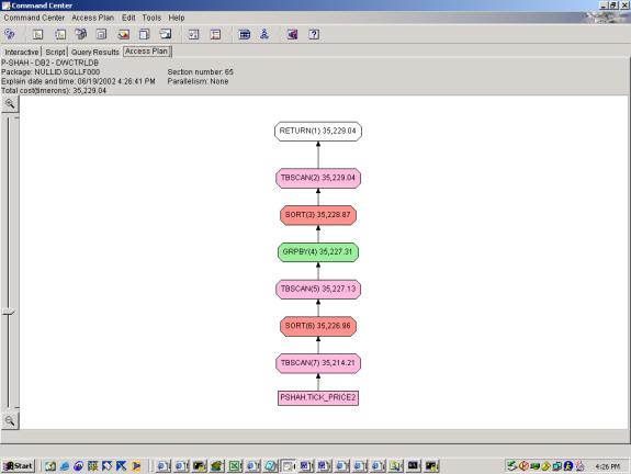
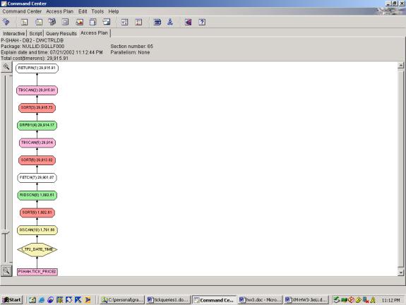
Syntax and Access Plans: 4 attempts were made at this simple query, which involves 1 aggregation, 1 predicate and a top ten filter. The first, Q4.1, shows the most basic access plan with a full table scan on the table, followed by the <sort, tablescan, group by> pattern to achieve the aggregation, and a final sort on the aggregated result. The plan is adequate, and under the circumstances, we cannot suggest a better one. Q4.2 improves on this due to the addition of an index on TRADEDATE, TIMESTAMP. 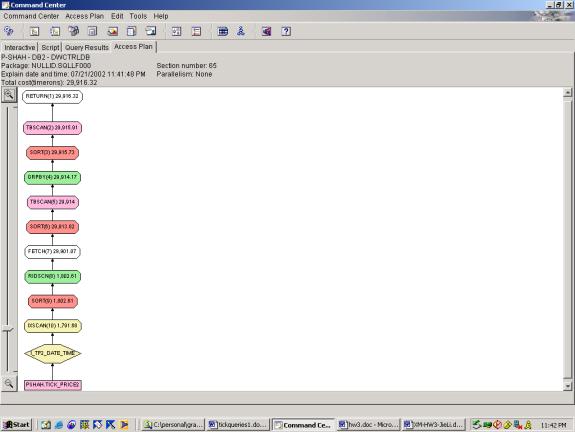The plan substitutes an INDEX SCAN + ROWiD LOOKUPS for the TABLE SCAN, and achieves 18% savings. 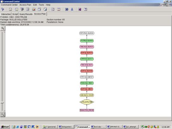Q4.3 adds a numerical rank to the query, but doesn’t change the access plan or cost estimate. Q4.4 adds a filter on the top ten ranks, causing the addition of a FILTER to the access plan – as expected.

--Q4.1 TOP TEN ACTIVE STOCKS (NO INDEXES, CLIENT SIDE TOP TEN FILTER)

SELECT sum(tradesize), id

FROM tick_price2

WHERE tradedate='06/13/2002'

GROUP BY id

ORDER BY sum(tradesize) DESC

--Q4.2 TOP TEN ACTIVE STOCKS (INDEXES, CLIENT SIDE TOP TEN FILTER)

SELECT sum(tradesize), id

FROM tick_price2

WHERE tradedate='06/13/2002'

GROUP BY id

ORDER BY sum(tradesize) DESC

--Q4.3 TOP TEN ACTIVE STOCKS (INDEXES, CLIENT SIDE TOP TEN FILTER, USES OVER)

SELECT id, rank() OVER (ORDER BY sum(tradesize))

FROM tick_price2

WHERE tradedate='06/13/2002'

GROUP BY id

--Q4.4 TOP TEN ACTIVE STOCKS (INDEXES, TOP TEN FILTER INCLUDED, USES OVER)

WITH

allids (id, rank) AS

(SELECT id, rank() OVER (ORDER BY sum(tradesize))

FROM tick_price2

WHERE tradedate='06/13/2002'

GROUP BY id)

SELECT id

FROM allids

WHERE rank<11

Detailed Analysis: This query doesn’t reveal much new information about the optimizer’s abilities. Similar to Query 3, the top ten filter and ranking function adds very little cost to the overall plan. Also, the sequence of operations is as expected – there is no other way to generate the rank then to do it after the aggregation step since it depends on the results of the aggregation.

Query 5

Specification:

5.	Find the most active stocks in the "COMPUTER" industry (use SIC code)

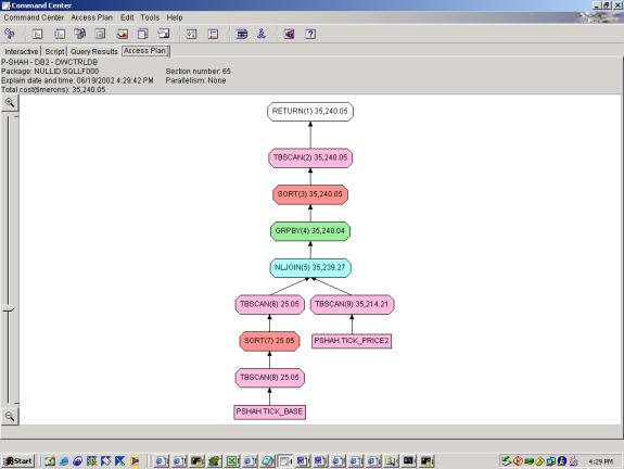
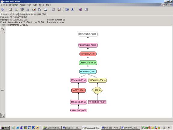
Syntax and Access Plans: Query 5 involves a join of two relations, 1 predicate, 1 aggregation, and an order on the aggregation result. Q5.1 is an efficient access plan under the circumstances, as it involves full tablescans on both TICK_PRICE2 and TICK_BASE2. The optimizer acknowledges that the second relation is much smaller than the first, and thus rightly chooses the nested loop join. Once joined, the aggregation is performed and its results are sorted. Interestingly, the filter on TICK_BASE.SIC is done within the TICK_BASE2 tablescan operation (not apparent from the picture, but apparent when we look at the detailed statistics). Thus, the subsequent aggregation only occurs on the ids that have SIC=COMPUTERS which is correct. Query 5.2 achieves significant cost savings (10 times less) by replacing the full table scan on TICK_PRICE2 with an index scan on TICK_PRICE2. 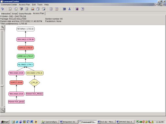Otherwise the query is very similar to its predecessor. 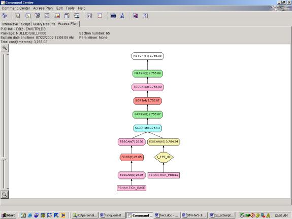Query 5.3 adds an explicit rank to the output using the OVER clause – the access plan and cost estimate are identical. Q5.4 adds a top ten filter (worth noting even though its not in the spec), which results in the addition of one filter at the end of the plan – no cost added.

--Q5.1 MOST ACTIVE STOCKS (NO INDEXES)

SELECT count(1),a.id

FROM tick_price2 a,

tick_bASe b

WHERE a.id=b.id

AND b.SIC='COMPUTERS'

GROUP BY a.id

ORDER BY count(1) DESC

--Q5.2 MOST ACTIVE STOCKS (INDEXES)

SELECT count(1),a.id

FROM tick_price2 a,

tick_bASe b

WHERE

a.id=b.id

AND b.SIC='COMPUTERS'

GROUP BY a.id

ORDER BY count(1) DESC

--Q5.3 MOST ACTIVE STOCKS (INDEXES, USES OVER)

SELECT a.id, rank() OVER (ORDER BY count(1) DESC)

FROM tick_price2 a,

tick_bASe b

WHERE

a.id=b.id

AND b.SIC='COMPUTERS'

GROUP BY a.id

--Q5.4 MOST ACTIVE STOCKS (INDEXES, USES OVER, TOP TEN FILTER INCLUDED)

WITH

allids (id, rank) AS (SELECT a.id, rank() OVER (ORDER BY count(1) DESC)

FROM tick_price2 a,

tick_bASe b

WHERE

a.id=b.id

AND b.SIC='COMPUTERS'

GROUP BY a.id)

SELECT id

FROM allids

WHERE rank < 11

Detailed Analysis: Query 5 demonstrates the ability of the Optimizer to use indexes, join two relations, and perform the rank function. As seen in attempts 5.3 and 5.4, the addition of the over clause and subsequent filtering on the over clause add very little overhead. The fact that 5.2 and 5.3 have identical access plans indicates that the over clause is handled exactly as an ORDER BY – rightly so. This query also demonstrates the ability of the optimizer to join 2 different relations – it handles this well as one relation is significantly smaller than the other and it uses a nested loop join. Also, the filter on SIC is pushed down to the below the join which results in significant cost savings.

Query 6

Specification:

6.	Find the 10 stocks with the highest percentage spreads. Spread is the difference between the last ask-price and the last bid-price. Percentage spread is calculated as a percentage of the mid-point price (average of ask and bid price).

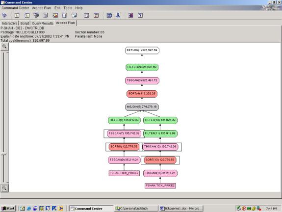
Syntax and Access Plans: Query 6 involves a calculation on 2 separate aggregations (max tradedate/timestamp where ask_price is not null and max tradedate/timestamp where bid_price is not null), with subsequent order on this calculation. 6.1 shows the best case query which achieves the correct results according to the specification. It still requires 2 full table scans on TICK_PRICE2 since the 2 aggregations are on different subsets of data – while the over clause allows for inline aggregations on different partitions of the same base data, it does not allow inline aggregations on different sets of base data. Thus, we cannot think of a way to reduce this query further. The optimizer rightly chooses the merge join since the two sets to be joined are of similar size. The final sort and filter are required since they act on the results of the joined data.

--Q6.1 HIGHEST PERC SPREAD (INDEXES, USES OVER, 2 TABLE SCANS ON TICK_PRICE2, TOP TEN FILTER INCLUDED, NO DATE FILTERS)

WITH

LAStB (id, bidprice, lASttime) AS

(SELECT id, bidprice, ROW_NUMBER() OVER (PARTITION BY id ORDER BY

tradedate,timestamp DESC) AS rown FROM Tick_price2

WHERE bidprice is not null),

LAStA (id,ASkprice, lASttime) AS

(SELECT id, ASkprice, ROW_NUMBER() OVER (PARTITION BY id ORDER BY

tradedate,timestamp DESC) rown FROM Tick_price2

WHERE ASkprice is not null),

allids (id, rank) AS

(SELECT a.id, rank() OVER (ORDER BY (2*(b.ASkprice-a.bidprice) / (b.ASkprice+a.bidprice)) DESC)

FROM

LAStB a, LAStA b

WHERE

a.id=b.id

AND a.lASttime=1

AND b.lASttime=1)

SELECT id

FROM allids

WHERE rank < 11

Detailed Analysis: While we do not show the progression, this query is similar to Query 3. Without the over clause we would potentially require 4 full table scans instead of 2. However, as stated in the previous section, we realize a limitation of the over clause in this query – we cannot perform inline aggregations on different sets of base data (see above for further explanation). The optimizer does well with the Over clause – treats it just as if it were an ORDER BY, and correctly merge joins the two similar-sized data sets. The final sort and filter are appropriate as they rely on the results of the join.

Markets

Query 1

Specification:

1	Get the closing price of a set of 10 stocks for a 10-year period and group into weekly, monthly and yearly aggregates. For each aggregate period determine the low, high and average closing price value. The output should be sorted by id and trade date.

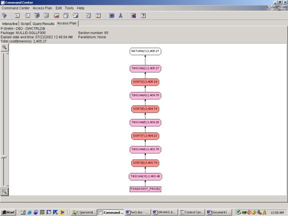
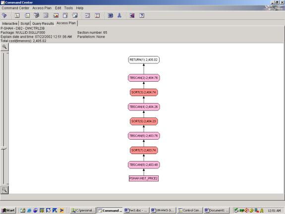
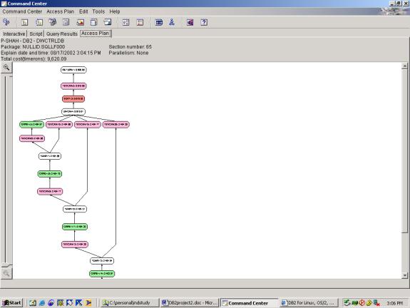
Syntax and Access Plan: Markets Query 1 involves 3 aggregations, over 3 different partitions, over the same base set of data. The first 2 attempts use the OVER clause and the last attempt uses the ROLLUP clause. Both achieve the results as stated in the specification. Q1.1 shows that the optimizer allows the sorts to be re-used in different aggregations of the same partition – which is correct. It also shows that sorts are able to build off of each other – that is, it performs the weekly, monthly and yearly sort with each one feeding into the next – which is also correct. Interestingly, in Q1.3, the rollup, although better suited for this query, results in a less efficient access plan. It seems to do each aggregation separately and then union the results rather than a sequential plan as in 1.2 and 1.1. Perhaps since the aggregates in this query are hierarchical – that is, they are all based on the same column, tradedate – the OVER clause performs better than ROLLUP.

--Q1.1 CLOSE PRICE OVER WEEK, MONTH, YEAR AGGREGATES (WITH ORDER)

SELECT

id,

tradedate,

max(closeprice) OVER (PARTITION BY id, month(tradedate)),

min(closeprice) OVER (PARTITION BY id, month(tradedate)),

avg(closeprice) OVER (PARTITION BY id, month(tradedate)),

max(closeprice) OVER (PARTITION BY id, year(tradedate)),

min(closeprice) OVER (PARTITION BY id, year(tradedate)),

avg(closeprice) OVER (PARTITION BY id, year(tradedate)),

max(closeprice) OVER (PARTITION BY id, week(tradedate)),

min(closeprice) OVER (PARTITION BY id, week(tradedate)),

avg(closeprice) OVER (PARTITION BY id, week(tradedate))

FROM

hist_price2

WHERE year(tradedate) = 2002

AND id LIKE '%_11%'

ORDER BY id, tradedate

--Q1.2 CLOSE PRICE OVER WEEK, MONTH, YEAR AGGREGATES (WITHOUT ORDER)

SELECT

id,

tradedate,

max(closeprice) OVER (PARTITION BY id, month(tradedate)),

min(closeprice) OVER (PARTITION BY id, month(tradedate)),

avg(closeprice) OVER (PARTITION BY id, month(tradedate)),

max(closeprice) OVER (PARTITION BY id, year(tradedate)),

min(closeprice) OVER (PARTITION BY id, year(tradedate)),

avg(closeprice) OVER (PARTITION BY id, year(tradedate)),

max(closeprice) OVER (PARTITION BY id, week(tradedate)),

min(closeprice) OVER (PARTITION BY id, week(tradedate)),

avg(closeprice) OVER (PARTITION BY id, week(tradedate))

FROM

hist_price2

WHERE year(tradedate) = 2002

AND id LIKE '%_11%'

--Q1.3 CLOSE PRICE OVER WEEK, MONTH, YEAR AGGREGATES (ROLLUP WITH ORDER)

SELECT

id,

year(tradedate),

month(tradedate),

week(tradedate),

max(closeprice),

min(closeprice),

avg(closeprice)

FROM

hist_price2

WHERE year(tradedate) = 2002

AND id LIKE '%_11%'

group by rollup ((id,year(tradedate)),

(id,month(tradedate)),

(id,week(tradedate)))

order by id, year(tradedate),

month(tradedate),

week(tradedate)

(top view)

(bottomview)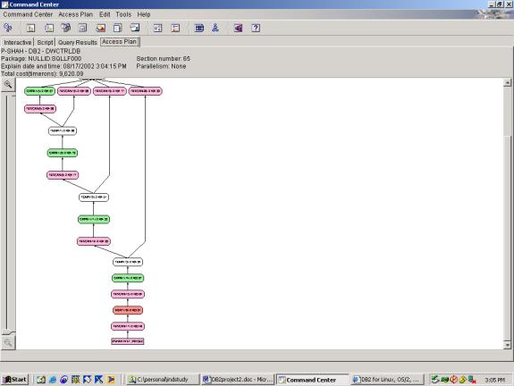

Detailed Analysis: The optimizer handles aggregations using the OVER clause very well in the case of 1.1. and 1.2. Since all aggregations build off the same column (tradedate), the optimizer is able to reuse the results of each sort. In the case of the ROLLUP in 1.3, the optimizer must perform the extra step of union-ing the results of each aggregation. This adds significant overhead.

Query 2

Specification:

2

Adjust all prices and volumes (prices are multiplied by the split factor and volumes are divided by the split factor) for a set of 1000 stocks to reflect the split events during a specified 300 day period, assuming that events occur before the first trade of the split date. These are called split-adjusted prices and volumes.

Syntax and Access Plan: Query 2 is complex at first, but greatly simplified with a little bit of high school math. Realizing that the PRODUCT() aggregate function can be substituted with:

Product x_i = exp (S ln (x_i))

We have an efficient plan that achieves the results required. As a sidenote, we initially approached this query by thinking about 1) the WITH RECURSIVE clause, and 2) User Defined Functions. However, we realized these costly options were not necessary as stated above. Query 2.1 involves 2 aggregations, 1 cartesian-outer join between different relations and 2 predicates. The plan scans both tables, and joins the results using a merge join.

--Q2.1 SPLIT ADJUSTED PRICE AND VOLUME

SELECT a.id,

tradedate,

value(exp(sum(ln(value(b.splitfactor,1)))),1) adj_split_factor,

closeprice*value(exp(sum(ln(value(b.splitfactor,1)))),1) adj_price,

volume / value(exp(sum(ln(value(b.splitfactor,1)))),1) adj_volume,

closeprice,

volume

FROM

hist_price2 a left outer join hist_split2 b

on a.id=b.id

AND a.tradedate<b.splitdate

WHERE a.id LIKE '%_1%'

AND year(tradedate)=2002

GROUP BY a.id, tradedate, closeprice, volume

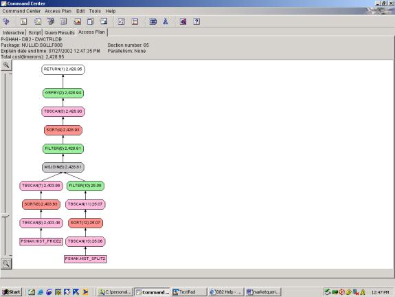
Detailed Analysis: The plan is adequate given the 2 relations and the Cartesian outer join. The optimizer chooses the merge join – possibly due to the Cartesian outer join - it does not have any concrete information on the size of the 2 data sets to be joined. Thus, is does not use a nested loop join here, which seems correct. It performs the aggregation <sort, tablescan, groupby> on the results of the join correctly. It handles order pretty well as can be seen by the 2 sorts in the subtrees – these sorts make the subsequent merge join more efficient.

Query 3

Specification:

3	For each stock in a specified list of 1000 stocks, find the differences between the daily high and daily low on the day of each split event during a specified period.

Syntax and Access Plans: Query 3 is simple – it involves selection from 2 joined relations with a single predicate. There is no aggregation or order. The optimizer does a full tablescan on both tables and then joins using a nested loop join. This makes sense because one relation is much smaller than the other.

--Q3.1 DAILY HI/LOW ON SPLITDATE

SELECT a.id, tradedate,

lowprice, highprice

FROM

hist_price2 a,

hist_split2 b

WHERE a.id=b.id

AND a.tradedate=b.splitdate

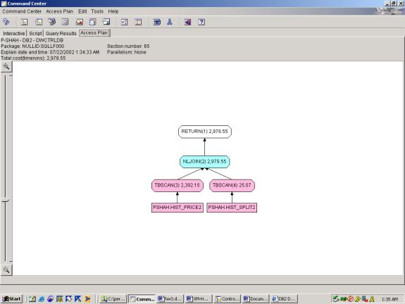
Detailed Analysis: The optimizer chooses the proper join method, and performs 2 full tablescans which is adequate given the requirements.

Query 4

Specification:

4	Calculate the value of the S&P500 and Russell 2000 index for a specified day using unadjusted prices and the index composition of the 2 indexes (see appendix for spec) on the specified day

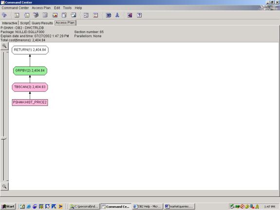
Syntax and Access Plans: Both parts of Query 4 requires 1 aggregation and 2 predicates. They have simple access plans which show a tablescan followed by a group by.

--Q4.1 RUSSELL AND SP INDICES -- AS TWO SEPARATE QUERIES

SELECT avg(closeprice) Russell200

FROM

hist_price2

WHERE tradedate='6/25/2002'

AND id LIKE 'Security_1%'

SELECT avg(closeprice) SP5

FROM

hist_price2

WHERE tradedate='6/25/2002'

AND id LIKE 'Security_10%'

Detailed Analysis: Query 4 is handled adequately by the optimizer – we cannot think of any better alternatives for the simple plan.

Query 5

Specification:

5	Find the 21-day and 5-day moving average price for a specified list of 1000 stocks during a 6-month period. (Use split adjusted prices)

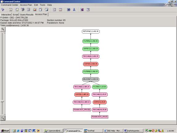
Syntax and Access Plans: Building off of Query 2, this query adds 2 aggregations with different windowing groups, and 2 predicates. The moving averages rely on the fact that the data in the Markets database is regular time series, hence the use of the ROWS clause. Query 5.1 shows the basic plan, while 5.2 and 5.3 attempt to show how well the optimizer pushes down the filters. In all three cases, the ID filter and YEAR filter occur as part of the first tablescan on HIST_PRICE2. The subsequent operations, until the join, are the same as Query 2. In all three cases, there is a filter and a group by operation after the join.

--Q5.1 21 DAY AND 5 DAY MOVING AVG.

WITH

splitadj (id, tradedate, adjprice, adjvolume) as (SELECT a.id,

tradedate, closeprice*value(exp(sum(ln(value(b.splitfactor,1)))),1) adj_price,

volume / value(exp(sum(ln(value(b.splitfactor,1)))),1) adj_volume

FROM

hist_price2 a left outer join hist_split2 b

on a.id=b.id

AND a.tradedate<b.splitdate

WHERE a.id LIKE '%_1%'

AND year(tradedate)=2002

GROUP BY a.id, tradedate, closeprice, volume)

SELECT

id,

tradedate,

avg(adjprice) OVER (PARTITION BY id ORDER BY tradedate asc ROWS between 21 preceding AND current row) day21,

avg(adjprice) OVER (PARTITION BY id ORDER BY tradedate asc ROWS between 5 preceding AND current row) day5

FROM

splitadj

WHERE

id LIKE 'Security_1%'

AND year(tradedate)=2002

--Q5.2 21 DAY AND 5 DAY MOVING AVG. (compare to Q5.3 – shows push down ability)

WITH

splitadj (id, tradedate, adjprice, adjvolume) as (SELECT a.id,

tradedate, closeprice*value(exp(sum(ln(value(b.splitfactor,1)))),1) adj_price,

volume / value(exp(sum(ln(value(b.splitfactor,1)))),1) adj_volume

FROM

hist_price2 a left outer join hist_split2 b

on a.id=b.id

AND a.tradedate<b.splitdate

GROUP BY a.id, tradedate, closeprice, volume)

SELECT

id,

tradedate,

avg(adjprice) OVER (PARTITION BY id ORDER BY tradedate asc ROWS between 21 preceding AND current row) day21,

avg(adjprice) OVER (PARTITION BY id ORDER BY tradedate asc ROWS between 5 preceding AND current row) day5

FROM

splitadj

WHERE

id LIKE 'Security_1%'

AND year(tradedate)=2002

--Q5.3 21 DAY AND 5 DAY MOVING AVG. (compare to Q5.2 – shows push down ability)

WITH

splitadj (id, tradedate, adjprice, adjvolume) as (SELECT a.id,

tradedate, closeprice*value(exp(sum(ln(value(b.splitfactor,1)))),1) adj_price,

volume / value(exp(sum(ln(value(b.splitfactor,1)))),1) adj_volume

FROM

hist_price2 a left outer join hist_split2 b

on a.id=b.id

AND a.tradedate<b.splitdate

WHERE

a.id LIKE 'Security_1%'

AND year(a.tradedate)=2002

GROUP BY a.id, tradedate, closeprice, volume)

SELECT

id,

tradedate,

avg(adjprice) OVER (PARTITION BY id ORDER BY tradedate asc ROWS between 21 preceding AND current row) day21,

avg(adjprice) OVER (PARTITION BY id ORDER BY tradedate asc ROWS between 5 preceding AND current row) day5

FROM

Splitadj

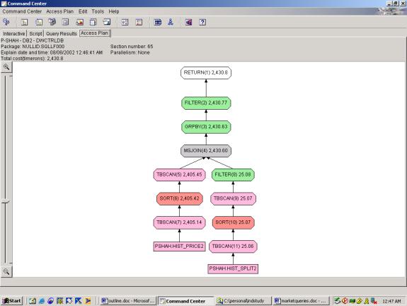
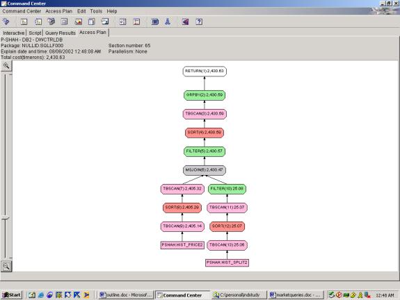
Detailed Analysis: Query 5.1 makes it easy on the optimizer by putting the filters in both the subquery and outer query. Query 5.2 keeps the filters in the outer query only, and 5.3 keeps the filters in the subquery only. In all cases the relative cost is the same. Thus, it seems to be successfully pushing down filters in this case. Looking at more detail, we see that Query 5.3 applies the YEAR filter three times. In Query 5.2, it is applied twice. In Query 5.1, it is applied once. So, even though the cost estimates show that all three have the same cost, we can see that there are the least steps taken in Query 5.1. The first half of the access plan (through the MSJOIN) is identical to Query 2 – see comments above on the optimizer analysis. The grouping operation takes care of both aggregations (5 day and 21 day) – which is correct.

Query 6

Specification:

6	(Based on the previous query) Find the points (specific days) when the 5-month moving average intersects the 21-day moving average for these stocks. The output is to be sorted by id and date.

Syntax and Access Plan: Query 6 builds from Query 5. It simply adds 1 aggregation and a new predicate. Interestingly, the added calculations result in a lower cost plan, and there is no extra work for the aggregation, and the new predicate is calculated at the end after the aggregation – which is correct since the predicate is dependent on the aggregation.

--Q6.1 21 DAY AND 5 DAY POINTS OF INTERSECTION

WITH

splitadj (id, tradedate, adjprice, adjvolume) as (SELECT a.id,

tradedate, closeprice*value(exp(sum(ln(value(b.splitfactor,1)))),1) adj_price,

volume / value(exp(sum(ln(value(b.splitfactor,1)))),1) adj_volume

FROM

hist_price2 a left outer join hist_split2 b

on a.id=b.id

and a.tradedate<b.splitdate

WHERE a.id like '%Security_1%'

and year(tradedate)=2002

GROUP BY a.id, tradedate, closeprice, volume),

mov21_5 (id, tradedate, day21, day5)

as (SELECT id, tradedate, avg(adjprice) over (PARTITION BY id order by tradedate asc ROWS between 21 preceding and current row) day21,

avg(adjprice) over (PARTITION BY id order by tradedate asc ROWS between 5 preceding and current row) day5

FROM

splitadj),

mov21_5cross (id, tradedate, day21prev, day5prev)

as

(SELECT id, tradedate, avg(day21) over (PARTITION BY id order by tradedate rows between 2 preceding and 1 preceding),

avg(day5) over (PARTITION BY id order by tradedate rows between 2 preceding and 1 preceding),

day21,

day5

FROM mov21_5)

SELECT *

FROM mov21_5cross

WHERE sign(day21-day5)*sign(day21prev-day5prev) < 0

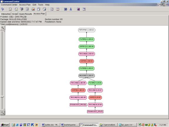
Detailed Analysis: Query 6 builds from Query 5 and Query 2. The plan is identical to Query 5 except that it includes an extra filter at the end to accommodate the new predicate. This filter must come at the end because it is dependent on the results of the aggregation. The optimizer pushes down filters well in this case.

Query 8

Specification:

8	Find the pair-wise coefficients of correlation in a set of 10 securities for a 2 year period. Sort the securities by the coefficient of correlation, indicating the pair of securities corresponding to that row. [Note: coefficient of correlation defined in appendix]

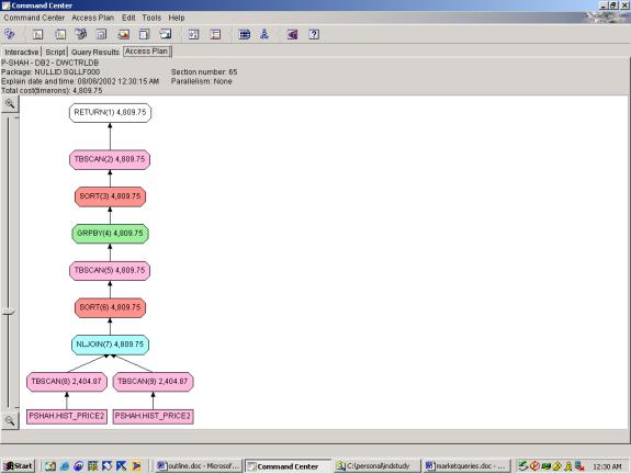
Syntax and Access Plans: Query 8 involves a Cartesian join between 2 relations, with 1 aggregate function and an ordering on the aggregation. The optimizer chooses a nested loop join followed by the group by pattern <sort, tablescan, groupby>, followed by a sort. The aggregation must occur after the join and the sort must occur after the aggregation since each depends on the last operation.

--Q8.1 PAIR WISE COEFFICIENTS

SELECT

a.id,

b.id,

correlation(a.closeprice, b.closeprice)

FROM

(SELECT * FROM hist_price2 WHERE id LIKE 'Security_10%' AND (tradedate='6/25/2002' or tradedate='6/26/2002' or tradedate='6/27/2002')) a,

(SELECT * FROM hist_price2 WHERE id LIKE 'Security_20%' AND (tradedate='6/25/2002' or tradedate='6/26/2002' or tradedate='6/27/2002')) b

WHERE

a.tradedate=b.tradedate

group by a.id, b.id

order by correlation(a.closeprice, b.closeprice)

Detailed Analysis: Query 8 involves a Cartesian join between 2 relations of equal size. The 2 relations are subqueries with 1 predicate each. The filters are performed as part of the tablescan, correctly. The optimizer chooses a nested loop join – however the 2 relations are of equal size. We believe that a merge join would have been better here. Next, it performs the aggregation, and sorts the results of the aggregation – which is satisfactory.

Query 9

Specification:

9	Determine the yearly dividends and annual yield (dividends/average closing price) for the past 3 years for all the stocks in the Russell 2000 index that did not split during that period. Use unadjusted prices since there were no splits to adjust for.

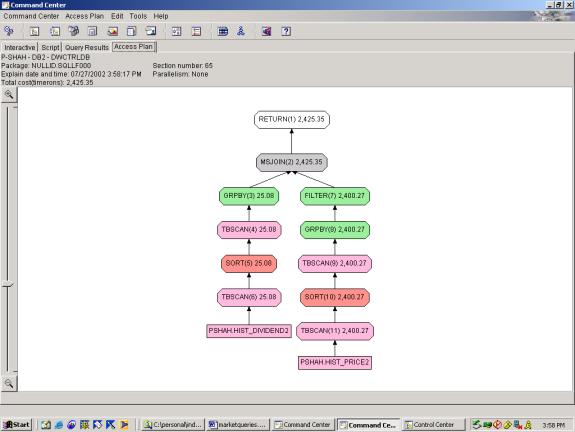
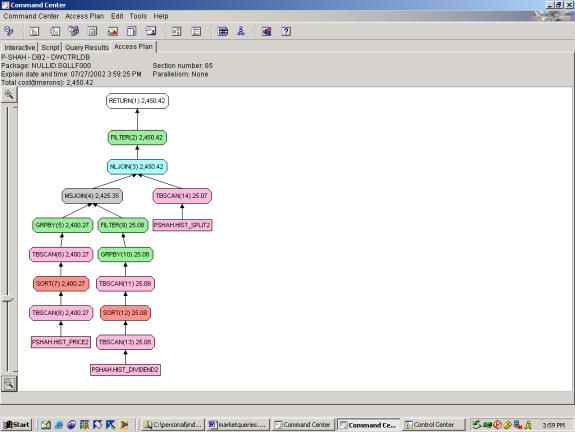
Syntax and Access Plan: Query 9 is a selection from 2 joined relations with 3 predicates. The 2 relations are subqueries which each have 1 predicate and 1 aggregation. The access plan for 9.1 shows a full tablescan on each relation, followed by the aggregation, followed by a merge join. In 9.2, we add the criteria that the security did not have any splits – this introduces a third relation. In 9.2, the access plan shows a full tablescan on each relation, followed by the aggregation, followed by a merge join – next, there is an outer join with the 3^rd relation – for which the optimizer chooses the nested loop join.

--Q9.1 YEARLY DIVIDENDS AND ANNUAL YIELD (SELECTS ALL – NOT JUST SECURITIES THAT HAVE NOT HAD SPLITS). CHANGED THIS TO MONTHLY DIV AND MONTHLY YIELD B/C OF SMALLER SET OF DATA

SELECT

a.id,

a.totaldiv as month_divs,

a.totaldiv / b.avgprice as month_yield

FROM

(SELECT id, sum(divamt) totaldiv FROM hist_dividend2 WHERE month(divdate)=7 GROUP BY id) a,

(SELECT id, avg(closeprice) avgprice FROM hist_price2 WHERE month(tradedate) = 7 GROUP BY id) b

WHERE a.id=b.id

AND (a.id = 'Security_2' or a.id = 'Security_3') -- as Russell index criteria

(should be SELECTing not split adjusted) / additional criteria in spec

--Q9.2 YEARLY DIVIDENDS AND ANNUAL YIELD (SELECTS ONLY SECURITIES THAT HAVE NOT HAD SPLITS) CHANGED THIS TO MONTHLY DIV AND MONTHLY YIELD B/C OF SMALLER SET OF DATA

SELECT

a.id,

a.totaldiv as month_divs,

a.totaldiv / b.avgprice as month_yield

FROM

(SELECT id, sum(divamt) totaldiv FROM hist_dividend2 WHERE month(divdate)=7 GROUP BY id) a,

(SELECT id, avg(closeprice) avgprice FROM hist_price2 WHERE month(tradedate) = 7 GROUP BY id) b

WHERE a.id=b.id

AND (a.id = 'Security_2' or a.id = 'Security_3')

AND not exists (SELECT 'x' FROM hist_split2 c

WHERE c.id=a.id)

Detailed Analysis: In Query 9.1, the optimizer performs adequately. It chooses the merge join for 2 equal size relations. However, in query 9.2 it applies the outer join with HIST_SPLIT2 after the merge join. We feel that this would be more efficient if applied before the merge join – it would lessen the amount of rows to be merge joined.

Test Results Summary

The tables below show a summary of the best-case plans for each query. For detailed query rewrite attempts and access plans, please see Test Results Detail.

Query Syntax

The following tables show, for each data model, the relative readability and development effort involved for each of the best-case queries.

Readability categories are: Simple – uses basic SQL constructs for the purposes intended and no mathematical formulas or “work-arounds” to achive the reuslts, Average – uses basic SQL constructs including SQL 99 additions for purposes intended and no mathematical formulas, Complex – uses mathematical formulas or “work arounds” to achieve desired results.

Development categories are: Easy – a person with knowledge of SQL92 can write the query with less than 3 attempts, Average – a person with detailed knowledge of SQL92 and basic knowledge of SQL99 can write the query with less than 3 attempts, Difficult – a person with detailed knowledge of SQL92, SQL99 and mathematical formulas can write the query in less than 10 attempts.

Ticks Database

Query	Query Type	Query Readability	Query Development
Q1.2	Simple Selection from Single Table with 3 Predicates	Simple	Easy
Q2.2	Selection from Single Table with 3 Predicates and 1 Aggregation	Simple	Easy
Q3.1	Top Ten Filter, 3 Aggregate Functions on different partitions, Selection on a Single Table, 3 Subqueries – each building on the last. Uses an OVER clause.	Complex	Difficult
Q4.4	1 Aggregation, Top Ten Filter, 1 Predicate. Uses an OVER clause.	Simple	Average
Q5.4	Ordering on Aggregate, Table Join on Primary Key, 1 Predicate, 1 Aggregation. Uses an OVER clause.	Average	Difficult
Q6.4	Top Ten Filter, 2 Aggregate functions on 2 different subsets of data. Selection on a single Table. 3 SubQueries building on each other. Uses an OVER clause.	Complex	Difficult

Markets Database

Query	Query Type	Query Readability	Query Development
Q1.1	3 Aggregate Functions on Different Time Periods, Selection on Single Table, 2 Predicates, SORT on result set. Uses an OVER clause.	Simple	Average
Q2.1	Selection on 2 Tables - Outer Joined, 2 Aggregate Functions, 2 Predicates.	Complex	Difficult
Q3.1	Selection on 2 Tables – Joined.	Simple	Simple
Q4.1	Selection on Single Table, 1 Aggregate Function, 2 Predicates	Simple	Simple
Q5.3	2 Aggregate Functions on different partitions, Single Subquery which includes 1 Aggregate Function and an Outer Join of 2 Tables, 2 Predicates. Uses an OVER clause.	Complex	Difficult
Q6.1	Building on Query 5, this one adds 2 additional Aggregate Functions on different partitions. It also adds a Predicate. Uses an OVER clause.	Complex	Difficult
Q8.1	1 Cartesian join, 1 aggregate function, 1 sort.	Complex	Average
Q9.2	Selection on 2 Subqueries, each involving different aggregate functions and inner joined. 1 Predicate and 1 NOT EXISTS.	Complex	Difficult

Query Optimization

The tables below show the Optimizer performance for each of the best-case queries for the Ticks and Markets databases. Cost Optimization ratings are Poor – we can find a better plan, Average – we cannot find a better plan but the optimizer does what we expect it to do, Excellent – we cannot find a better plan and the optimizer uses a particularly creative approach that we would not have expected. Total Cost is in units of timerons, and ratings are: Low <5k, Medium between 5k and 15k, High >15k.

Ticks Database

Query	Query nnnnnnssc Type	Total Cost	Join Method and Join Order	Sort Order	Selection Method	Application of Filters
Q1.2	Simple Selection from Single Table with 3 Predicates. Not ORDER Dependent.	12711 Medium	None	No explicit sort, however the optimizer SORTS the result of the INDEX SCAN on ROWID prior to looking up rows. This is very smart because it saves multiple lookups to the same page (which would be the case if it was not sorted on ROWID). Excellent.	Uses 2 Index Scans, and ANDs the result. Average.	None
Q2.2	Selection from Single Table with 3 Predicates and 1 Aggregation. Not ORDER Dependent.	12697 Medium	None	Same as Q1.2. Excellent.	Same as Q1.2. Average.	None
Q3.1	Top Ten Filter, 3 Aggregate Functions on different partitions, Selection on a Single Table, 3 Subqueries – each building on the last. Order Dependent. Uses OVER.	45025 High	Nested Loop Join with Literal Table Average	2 Sorts – One on ID and Tradedate (single sort for 2 grouping functions). The second sort is on PercentageLoss (couldn’t’ be pushed down because its dependent on an aggregate). Because we eliminated all except on full tablescan (and hence all joins), we also eliminated extraneous SORTS – a huge cost savings. The rationale of the attempts was essentially to reduce joins. A clustering index over ID and tradedate potentially eliminates the first sort. Excellent	Uses a Table Scan. Could have used an Index Scan. Its not clear why it fails to use the INDEX. Possibly due to the introduction of the Literal Table. Poor	2 Filters – One on Rank (couldn’t be pushed down because its dependent on an aggregate). The second filter is on Tradedate – this could have been pushed down but wasn’t. Since the TRADEDATE filter reduces the number of records significantly, this query is greatly adversely affected by the fact that the filter is not pushed down. Poor
Q4.4	Selection from Single Table, 1 Aggregation Top Ten Filter, 1 Predicate. Order Dependent. Uses OVER.	29916 High	None	There are 3 SORTS, (i) The first is similar to Q1.2. Excellent, (ii) the second is part of the aggregation pattern where we group on ID to get the rank – however, why sort again on ID when it was already sorted on ID in the first sort Poor, (iii) the third sort sorts on the result of the rank which must occur at the end, as expected Average	Uses Index. Average.	Filter is applied at the end. It is not possible to push down because it depends on the result of the aggregate. As expected. Average.
Q5.4	Ordering on Aggregate, Table Join on Primary Key, 1 Predicate, 1 Aggregation. Order Dependent. Uses OVER.	3755 Low	Nested Loop Join between ID Index on Tick_Price2 and Tick_Base. Average	Clever SORT is implemented after the Tick_Base TableScan – this aids the Nested Loop Join between Tick_Base and Tick_Price2. Excellent	Uses Index on Tick_Price2, and TableScan on Tick_Base. Average	Filter is applied at the end (could not push down because it depends on the result of the rank). Average
Q6.4	Top Ten Filter, 2 Aggregate functions on 2 different subsets of data. Selection on a single Table. 3 SubQueries each building on each other. Order Dependent. Uses OVER.	59875 High	Merge Join Between Each Copy of the Index Scan on Tick_Price2. This is an efficient Join method for 2 sorted sets of data relatively equal in size. Even though the sources are not originally sorted, the nested loop join is close to O(n^2), while the merge join is O(nlogn) Excellent.	Clever Sorts Are Inlcuded in two places: (i) After IndexScan Before ROWID Lookup, (ii) After TableScan, and Before MS JOIN. It is clever for the same reason as Q1.2 - Each of these makes the next step more efficient by reducing the number of disk reads when performing the ROWID lookup in (i), and when performing the join. Excellent	2 Index Scans on Tick_Price2. Average	4 Filters: (i) Filter on Rank – must be done at the end due to dependence on aggregate result Average, (ii) Filter on Ask Price – why not do this prior to the Second SORT thereby reducing the number of elements to join Poor (iii) Filter on Bid Price – why not do this prior to Second SORT – thereby reducing the number of elements to join Poor, (iv) Filter on Join. Average

Markets Database

Query	Query Type	Total Cost	Join Method and Join Order	Sort Order	Selection Method	Application of Filters
Q1.1	3 Aggregate Functions on Different Time Periods, Selection on Single Table, 2 Predicates, SORT on result set. Order Dependent. Uses OVER.	2405 Low	None	3 Separate Sorts for the 3 Aggregate Functions. We can’t think of any way around this. Final Sort for ID, Tradedate. This could have been pushed down, but wasn’t. Average	Table Scan on Hist Price2. Average	None
Q2.1	Selection on 2 Tables - Outer Joined, 2 Aggregate Functions, 2 Predicates Order Dependent.	2430 Low	Merge Join Between SPLIT2 and HIST2. Average	2 SORTS: (i) one sort prior to the Merge Join. Average (ii) one is part of the Group BY Pattern as expected. Average	2 TableScans which is as expected. Average	None
Q3.1	Selection on 2 Tables – Natural Joined. NOT Order Dependent.	2980 Low	None	None	1 TableScan, as expected. Average	None
Q4.1	Selection on Single Table, 1 Aggregate Function, 2 Predicates. NOT Order Dependent.	2404 Low	Nested Loop Join. This is appropriate because SPLIT2 is much smaller than PRICE2. Average	None	2 TableScans (on PRICE2 and SPLIT2). As expected. Average	None
Q5.3	2 Aggregate Functions on different partitions, Single Subquery which includes 1 Aggregate Function and an Outer Join of 2 Tables, 2 Predicates. Order Dependent. Uses OVER.	2430 Low	Merge Join Between SPLIT2 and HIST2. Average	2 SORTS: (i) one sort prior to the Merge Join. Average (ii) one is part of the Group BY Pattern as expected. Average	2 TableScans which is as expected. Average	Filter (on Tradedate and ID) is Pushed Down – Q5.2 and Q5.3 demonstrate this ability. Excellent
Q6.1	Building on Query 5, this one adds 2 additional Aggregate Functions on different partitions. It also adds a Predicate. Order Dependent. Uses OVER.	2430 Low	Merge Join Between SPLIT2 and HIST2. Average	2 SORTS: (i) one sort prior to the Merge Join. Average (ii) one is part of the Group BY Pattern as expected. Average	2 TableScans which is as expected. Average	Filter selects cross points -at the end because it is dependent on the result of the subqueries. Average
Q8.1	Partial Cartesian Join Between Two Copies of a Single Table, One Aggregate Function. Order Dependent.	4809 Low	Nested Loop Join Between Two Copies of the Same Table. Why Nested Loops Here. We have no reason to believe one Copy is smaller than the other. A better approach is to SORT and then Merge Join. Poor	2 SORTS: (i) one is part of the Group BY Pattern as expected. Average (ii) sorts the correlation coefficient at the end, because it is dependent on the aggregate result. Average	2 TableScans which is as expected. Average	None
Q9.2	Selection on 2 Subqueries, each involving different aggregate functions and inner joined. 1 Predicate and 1 NOT EXISTS. Order Dependent.	2450 Low	Merge Join Between PRICE2 and DIVIDEND2. Nested Loop Join between the output of the above and SPLIT2. Average.	2 Sorts as part of the Group By. Average	Table Scan on all 3 tables. Average	2 Filters (i) one for the Join between PRICE2 and DIVIDEND Average, (ii) one for the NOT EXISTS Clause. Could have been pushed down. Poor

Analysis & Conclusions

Query Optimization

Pushing Down Selections

Markets Query Q5.2 and Q5.3 can be used to show how effective the DB2 query optimizer is at pushing down selections. By moving around the Predicates (on ID and TRADEDATE) from the subquery (in Q5.2) to the outer query (in Q5.3), we see that the Filter remains in the first TableScan. Thus it is successfully pushed down to the first table scan of the table.

Another example of successful push down is the fact that Markets Queries 2.1, 5.1 and 6.1 all have almost the exact same access plan, but they are increasingly complex version of the same query. Since 6.1 has significantly more sophisticated calculations (and essentially builds off of 5.1 and 2.1), one would expect it to have a higher cost or more complex plan. The fact that it does not shows that much of the incremental work is pushed down so that there is very little extra overhead.

Choosing Join Order

Markets Query Q9.2 can be used to show how the DB2 performs when picking the join order. The three tables involved are SPLIT2, PRICE2 and DIVIDEND2 – SPLIT2 and DIVIDEND2 are obviously smaller and less costly to read and sort than PRICE2. The query requires a natural join between PRICE2 and DIVIDEND2 (JOIN1), and an anti-join (or not exists) between DIVIDEND2 and SPLIT2 (JOIN2). Since the anti-join appears to limit the set of data substantially, one would expect the SPLIT2 to DIVIDEND2 join to occur first, and the result to be joined to PRICE2. This would minimize the total cost of the expensive PRICE2 join. Thus it does not seem to choose join order amongst 3 relations very well.

Choosing Join Method

With Markets Q8.1, DB2 does a poor job at selecting a Join Method. It chooses a Nested Loop Join, but given the relative sizes of the relations which are near-equal, a Merge Join would appear to be more efficient. On the other hand, it does a great job at selecting a Join Method with Ticks Q6.4 where it chooses a Merge Join since the sizes of the join relations are similar.

Choosing Selection Method

We can see how DB2’s optimizer performs at selection method by looking at Ticks Q1.2 and Ticks Q3.1. In the first case (Q1.2), DB2 does a Suitable Selection at utilizing both the DATE/TIME Index and the ID Index. While it does not contain an explicit join, it assesses that the IndexAnd of these two Index Scans will be less expensive than using a single Index or no Index at all. On the other hand, the second case (Q3.1) shows an instance where DB2 demonstrates Poor Selection. In the first subquery, it performs a full table scan on TICK_PRICE2 instead of using an Index Scan to filter on TradeDate.

In addition, the SQL 99 WITH clause provides for more efficient selection since it allows one subquery to reference the results of another subquery. An example of this benefit is Ticks Q3.1, in which we were able to go from 4 joins down to 1 join (and improve total cost significantly), as a direct result of WITH clause enhancement. This progression can be seen with the various incremental phases of Ticks Query 3 (3.1 to 3.10).

Choosing SORT Order

We can see the DB2 optimizer does have adequate SORT Order Management by looking at Ticks Q5.2 where a SORT is added on the left branch prior to the Nested Loop join. This SORT orders the set of Ids obtained in the TableScan of HIST_BASE, and the ordered set of Ids forms the outer loop of the Nested Loop Join.

Another case where DB2 demonstrates outstanding SORT Order Management is Ticks Q4.4. Apart from the explicit SORTs in the query, it adds a SORT after the IndexScan which causes the next step of row lookups to be more efficient. The SORT is on ROWID, and thus guarantees that all rows on the same page are “looked up” at once rather than out of sequence. Thus there are less disk reads and a more efficient query overall.

Specifically, the optimizer handles the OVER clause similar to the way that it handles ORDER Bys. As shown in Markets Q1.1, it is able to consolidate OVER aggregations on different partitions of the same data set. Thus, it does not “re-sort” the data for each aggregation, or for each partition. However, in the case that the base data sets are different , such as Ticks Query 6, we must use 2 tablescans – the OVER clause does not provide syntax for linear aggregations over 2 different base data sets. In summary, for the implementation provided, it demonstrates satisfactory OVER Clause Management – however, the addition of allowing aggregations over different base data sets would be helpful in the case of Query 6.

Query Readability & Development

Ticks Q3.1 and Markets Q2.1 are prime examples of queries with extremely poor readability and complex development effort. These cases show that windowed functions can only appear on the select clause; which inevitably forces one to use nesting for more complex queries. In addition one cannot use a windowed function as the argument of an aggregate one.

We realize that the benchmark requires sophisticated calculations, and only come to this conclusion after finding alternatives that would make these queries more readable. With Ticks Q3.1, we could substitute the following clause:

avg(tradeprice) OVER (PARTITION BY id ORDER BY tradedate ASc ROWS BETWEEN 2 preceding AND 1 preceding)

with:

last(tradeprice) OVER (PARTITION BY ID ORDER BY TRADEDATE ASC)

For Markets Q2.1, we would substitute the following clause which makes use of the mathematical function –

Product x_i = exp (S ln (x_i))

value(exp(sum(ln(value(b.splitfactor,1)))),1) adj_split_factor,

with:

value(product(b.splitfactor),1) adj_split_factor

Thus, by adding the LAST (and FIRST) & PRODUCT aggregate functions, we could greatly improve the readability and development of the Queries.

Ticks Q4.4, however, is an example of a readable query, with complex development effort that benefits from the SQL 99 standard impelementation in DB2. In this query, the WITH clause provides for cleaner isolation of the subquery than the standard FROM subquery. Further, the use of the WITH clause in conjunction with the RANK function is intuitive and could be comprehended by a person that is not familiar with the OLAP functions. It still requires a pretty sophisticated developer to construct the various components of the RANK.

An example of a readable query, with simple development effort is Markets Q8.1. The CORRELATION function hides the complexity of the calculations. It could be dangerous, however, since a novice developer may use the wrong arguments to the functions and provide incorrect results.

References

1. Database System Implementation, Hector Garcia-Molina et. al., p.1

2. Database System Implementation, Hector Garcia-Molina et. al., p.7

3. DB2 Online Help, http://www-3.ibm.com/cgi-bin/db2www/data/db2/udb/winos2unix/support/document.d2w/report?fn=db2v7s0olapfunc.htm

4. DB2 Online Help, http://publib.boulder.ibm.com/pubs/html/as400/v5r1/ic2924/index.htm?info/db2/rbafzmstintsel.htm

5. Database System Implementation, Hector Garcia-Molina et. al., p.238

6. Database System Implementation, Hector Garcia-Molina et. al., p343

7. Database System Implementation, Hector Garcia-Molina et. al., p362

8. Database System Implementation, Hector Garcia-Molina et. al., p381

9. Database System Implementation, Hector Garcia-Molina et. al., p.385

10. Database System Implementation, Hector Garcia-Molina et. al., p.393

11. Database System Implementation, Hector Garcia-Molina et. al., p.408

12. Database System Implementation, Hector Garcia-Molina et. al., p.409

13. http://www.cs.nyu.edu/cs/faculty/shasha/fintime.d/bench.html