3D Coordinate system WebGL exists in a 3D world: x goes to the right y goes up z goes forward (out of the screen) This is called a right hand coordinate system. For now we are going to be doing all of our work starting with the x,y plane. Specifically we will be working with a square that extends from -1 → +1 in both x and y.

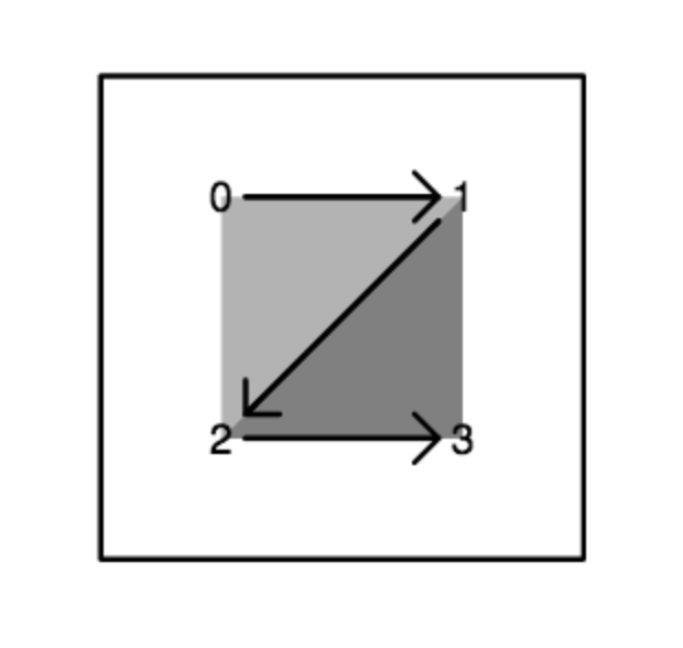
Square as a triangle strip Our geometry will be a square. In WebGL everything is made of triangles, so we will need two triangles. We define these as a triangle strip. In a triangle strip, every three successive vertices makes a new triangle, so we will need to specify a total of four vertices, as in the figure to the right.

Z-buffer algorithm The GPU (Graphics Processing Unit) renders using a "Z-buffer algorithm" For each animation frame, this algorithm consists of two successive steps: For each vertex: The GPU runs a vertex shader to: Find which pixel of the image contains this vertex; Set up "varying" values to be interpolated. For each triangle: The GPU interpolates from vertices to pixels. For each pixel: The GPU runs a fragment shader to: Compute color; If this is the nearest fragment at the pixel, replace color and depth at this pixel in the image.

Uniform variables GLSL (for "GL Shading Language") is the C-like language that is used for shaders on the GPU. One of its key constructs is a uniform variable. Uniform variables on the GPU have the same value at every pixel. They can (and often do) change over time. By convention, a uniform variable name starts with the letter 'u'. For your assignment, I have create some useful uniform variables: float uTime; // time elapsed, in seconds vec3 uCursor; // mouse position and state // uCursor.x goes from -1 to +1 // uCursor.y goes from -1 to +1 // uCursor.z is 1 when mouse down, 0 when mouse up.

Vertex shaders A vertex shader is a program that you (the application programmer/artist) writes which gets run on the GPU at every vertex. It is written in the special purpose language GLSL. To the right is a very simple vertex shader program. An "attribute" is a constant value that is passed in from the CPU. In this case, it is aPosition, the x,y,z position of each vertex in the scene. wIt is of type vec3, which means that it consists of three GLSL floating point numbers.

attribute vec3 aPosition; varying vec3 vPosition; void main() { gl_Position = vec4(aPosition, 1.0); vPosition = aPosition; }

One of the most powerful things that a vertex shader can do is set "varying" variables. These values are then interpolated by the GPU across the pixels of any triangles that use this vertex. That interpolated value will then be available to fragment shaders at each pixel. For example, "varying" variable vPosition is set by this vertex shader. By convention, the names of varying variables start with the letter 'v'. This vertex shader does two things: By setting gl_Position, it determines at which pixel of the image this vertex will appear. It sets varying variable vPosition to equal the attribute position aPosition for this vertex.

Fragment shaders A fragment shader is a program that you (the application programmer) writes which is run at every pixel. Because pieces of different triangles can be visible at each pixel (eg: when triangles are very small, or pixels where an edge of one triangle partly obscures another triangle), in general we are really defining the colors of fragments of pixels, which is why these are called fragment shaders. Since our vertex shader has set a value for vPosition, any fragment shader we write will be able to make use of this variable, whose values will now have been interpolated down to the pixel level.

Guides to WebGL There are many guides on-line to WebGL. I find this Tutorial on WebGL Fundamentals to be particularly clear and easy to follow for people who are new to WebGL. I also find this Quick Reference Card to be very useful when writing WebGL shaders. I think you will find the list of built-in functions on the last page to be particularly useful.

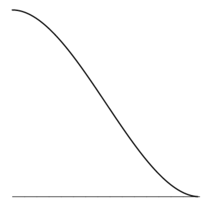
Gamma correction Displays are adjusted for human perception using a "gamma curve", since people can perceive a vary large range of brightness. For example, the image to the right shows the values 0...255 on the horizontal axis, the resulting actual displayed brightness on the virtual axis. Various displays differ, but this adjustment is generally approximately x2 Since all of our calculations are really summing actual photons of light, we need to do all our math in linear brightness, and then do a gamma correction when we are all finished: Roughly: c → sqrt(c)

Output brightness

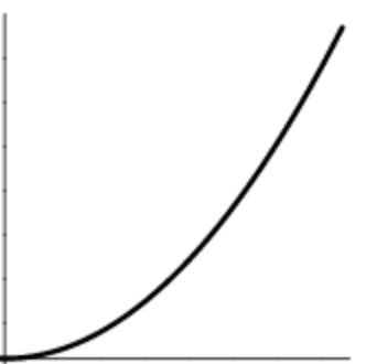
Input values 0 ... 255

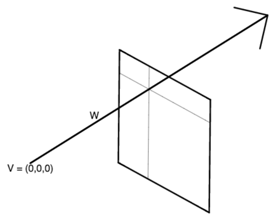
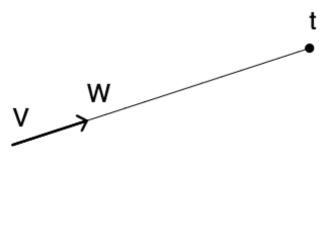
Ray tracing: Forming a ray At each pixel, a ray from the origin V = (0,0,0) shoots into the scene, hitting a virtual screen which is on the z = -f plane. We refer to f as the "focal length" of this virtual camera. The ray toward any pixel aims at: (x, y, -f), where -1 ≤ x ≤ +1 and -1 ≤ y ≤ +1. So the ray direction W = normalize( vec3(x, y, -f) ). Note that normalize() is a built-in function for OpenGL ES. In order to render an image of a scene at any pixel, we need to follow the ray at that pixel and see what object (if any) the ray encounters first. In other words, the nearest object at a point V + Wt, where t > 0.

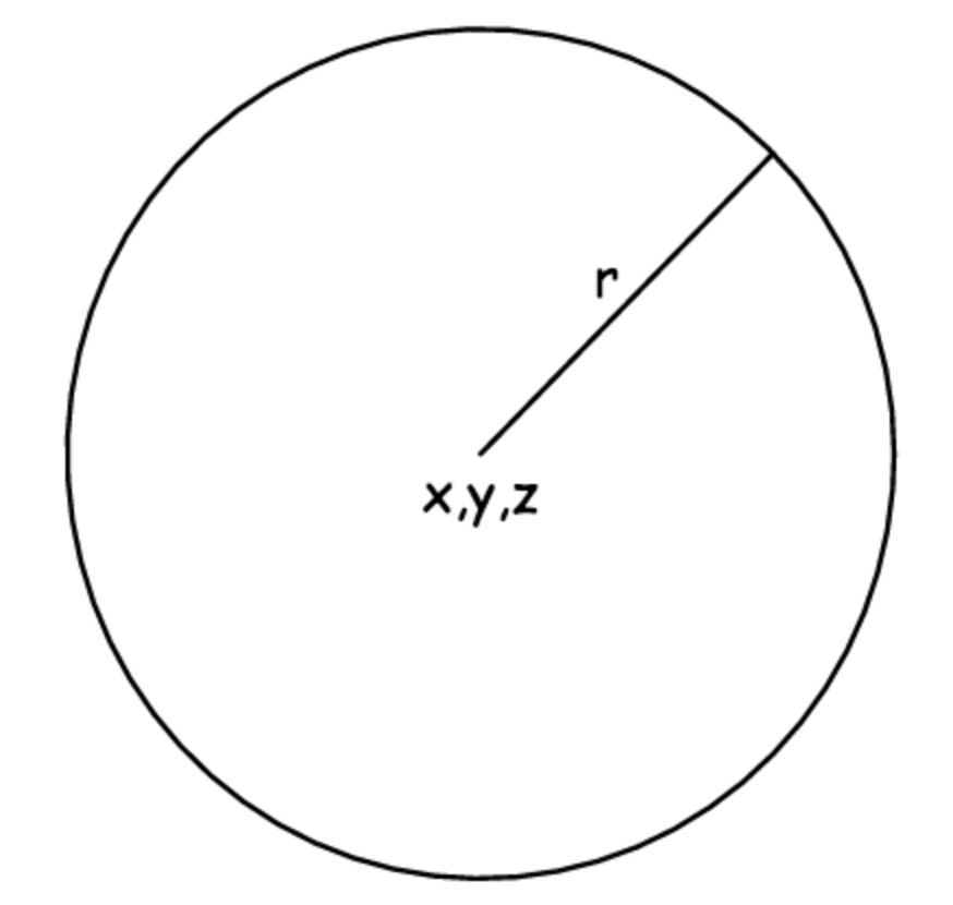
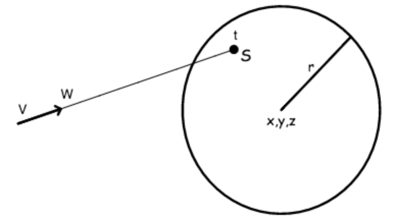
Ray tracing: Defining a sphere                                                                                                                                                                                                 We can describe a sphere in a GLSL vector of length 4: vec4 sphere = vec4(x,y,z,r); where (x,y,z) is the center of the sphere, and r is the sphere radius. As we discussed in class, the components of a vec4 in GLSL can be accessed in one of two ways: v.x, v.y, v.z, v.w // when thought of as a 4D point v.r, v.g, v.b, v.a // when thought of as a color + alpha So to access the value of your sphere's radius in a fragment shader vec4, you will want to refer to it as sphere.w (not sphere.r).

Ray tracing: Finding where a ray hits a sphere D = V - sph.xyz // vector from center of sphere to ray origin. The point of doing this subtraction is that we are then effectively solving the much easier problem of ray tracing to a sphere at the origin (0,0,0). So instead of solving the more complex problem of tracing a ray V+Wt to a sphere centered at sph.xyz, we are instead solving the equivalent, but much simpler, problem of tracing the ray D+Wt to a sphere centered at (0,0,0). (D + Wt)2 = sph.r2 // find a point along ray that is distance r from sphere center. (D + Wt)2 - sph.r2 = 0 // need to solve for t. Generally, if a and b are vectors, then a • b = ( ax * bx + ay * by + az * bz ) This "inner product" also equals: |a| * |b| * cos(θ) Multiplying the terms out, we need to solve the following quadratic equation: (W • W) t2 + 2 (W • D) t + (D • D) - r2 = 0 Since ray direction W is unit length, the first term in this equation (W • W) is just 1.

Ray tracing: Finding the nearest intersection Compute the intersection to all spheres in the scene. The visible sphere at this pixel, if any, is the one with smallest positive t.

Ray tracing: Computing the surface point Once we know the value of t, we can just plug it into the ray equation to get the location of the surface point on the sphere that is visible at this ray, as shown in the equation below and in the figure to the right: S = V + W t

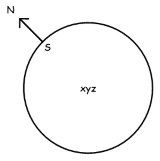
Ray tracing: Computing the surface normal We now need to compute the surface normal in order to compute how the sphere interacts with light to produce a final color at this pixel. The "surface normal" is the unit length vector that is perpendicular to the surface of the sphere -- the "up" direction if you are standing on the surface. For a sphere, we can get this by subtracting the center of the sphere from the surface point S, and then dividing by the radius of the sphere: N = (S - sph.xyz) / sph.r

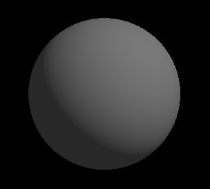
Ray tracing: A simple shader A simple light source at infinity can be defined as an rgb color, together with an xyz light direction: vec3 lightColor; // rgb vec3 lightDirection; // xyz A diffuse simple surface material can be defined by an rgb "ambient" component, which is independent of any particular light source, and an rgb "diffuse" component, which is added for each light source: vec3 ambient; // rgb vec3 diffuse; // rgb The figure to the right shows a diffuse sphere, where the point at each pixel is computed as: ambient + lightColor * diffuse * max(0, normal • lightDirection)

Ray tracing: Multiple light sources If the scene contains more than one light source, then pixel color for points on the sphere can be computed by: ambient + ∑n ( lightColorn * diffuse * max(0, normal • lightDirectionn) ) where n iterates over the lights in the scene.

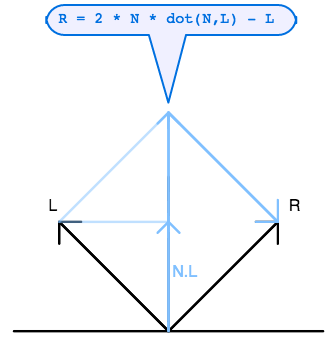
Phong model for specular reflection The first really interesting model for surface reflection was developed by Bui-Tong Phong in 1973. Before that, computer graphics surfaces were rendered using only diffuse lambert reflection. Phong's was the first model that accounted for specular highlights. The Phong model begins by defining a reflection vector R, which is a reflection of the direction to the light source L about the surface normal N. As we showed in class, and as you can see from the diagram on the right, it is given by: R = 2 (N • L) N - L

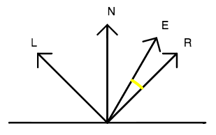
Once R has been defined, then the Phong model approximates the specular component of surface reflectance as: srgb max(0, E • R)p ) where srgb is the color of specular reflection, p is a specular power, and E is the direction to the eye (in our case, E = -W, the reverse of the ray direction). The larger the specular power p, the "shinier" the surface will appear. To get the complete Phong reflectance, we sum over the lights in the scene: argb + ∑i lightColori ( drgb max(0, N • Li) + srgb max(0, E • R) p ) where argb, drgb and srgb are the ambient, diffuse and specular color, respectively, and p is the specular power.

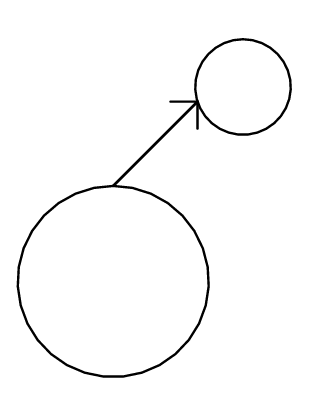
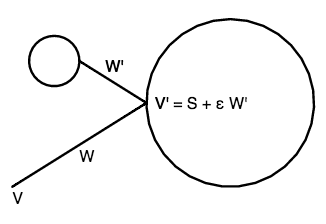
Shadows Casting shadows is relatively easy in ray tracing. Once we have found a surface point S, then for each light source, we shoot another ray whose origin V' is just the surface point S, and whose direction W' is the direction toward that light source Li. We want to make sure that the ray misses the object we are starting from, so we move the origin V' of our new ray slightly off the surface. Our "shadow ray" will therefore be: V' = S + ε Li W' = Li where ε is a very small positive number such as 0.001. If this shadow ray encounters any other object, then the surface is in shadow at this pixel, and we do not add in the diffuse and specular components of surface reflectance. To the right above is an example of the surface not being in shadow. Just below that is an example of a surface being in shadow, because its light path is blocked by another object. Implementation hint: As you loop through the light sources inside shadeSphere(), form a shadow ray at each iteration of the loop. Test that ray against every sphere in the scene to see whether there is a hit. If the ray has hit any sphere in scene, then don't add in diffuse or specular components from that light source.

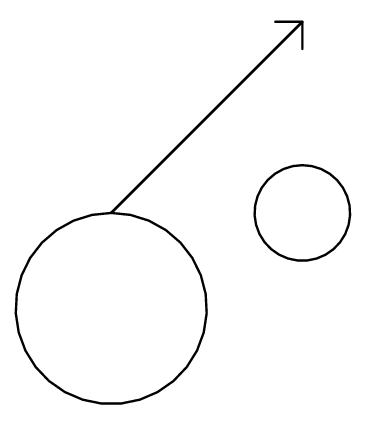
Reflection Another great thing about ray tracing is that we can continue to follow the path of a light ray backward from the camera, to model the behavior of mirror reflection. Adapting the technique that we used to calculate the reflection direction R for the Phong reflectance model, but replacing L in that equation by -W (the direction back along the incoming ray): W' = 2 (N • (-W)) N - (-W) we can compute a new ray that starts at surface point S, and goes into that reflected direction. As shown in the figure on the right, we want to offset the origin of this ray a bit out of the surface, so that the ray does not accidentally encounter the object itself. Whatever color is computed by this ray, we mix it into the result of the Phong reflectance algorithm. The result is the appearance of a shaded surface with a mirror finish.

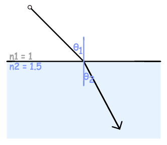
Refraction In the real world many materials, such as oil, water, plastic, glass and diamond, are transparent. A transparent material has an index of refraction which measures how much light slows down as it enters that medium. For example, the index of refraction of water is about 1.333, of glass is about 1.5. The index of refraction of diamond, the substance with the highest known index of refraction, is 2.42. As in the diagram to the right, you can add refraction to your ray tracing by following Snell's law: n1 / n2 = sin(θ2) / sin(θ1) to determine how much the ray should bend as it enters or exits a transparent object. Note that you will need to change your ray tracing model to incorporate refraction. In addition to your initial incoming ray, and any shadow or reflection rays, you also need to add a refraction ray, which starts just inside the surface, and continues inward. Note that if you have ray traced to a sphere, and are now computing where the refracting ray will exit that sphere, you will want to compute the second root of the quadratic equation. Then, after this refracting ray has exited out the back of the transparent sphere, you will want to compute how much it refracts on its way out, and then shoot a ray from there into the scene behind the sphere. In general, you use the results of refraction by mixing the color it returns together with whatever surface color you have computed due to pure reflection or blinn/phong reflectance.

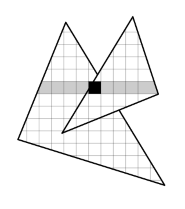
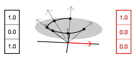
Homogeneous coordinates We can deal with both points in a scene and directions (which are essentially points at infinity) by adding an extra coordinate, which we call the homogeneous coordinate. For example, in two dimensions, we would write [x,y,w] to represent (x/w, y/w). In the example to the right, we have both points and directions. The point at (1,0) is represented by [1,0,1], whereas the direction vector (1,0) (shown in red) is represented by [1,0,0]. By convention we place all points on the w=1 plane (shown in gray), although scaling arbitrarily to [cx,cy,cw] still describes the same point (x/w, y/w), as shown by the upward slanting arrows in the figure. The same principle applies when we move to three dimensions: We use the homogeneous vector [x,y,z,w] to describe (x/w, y/w, z/w). • A point at location (x,y,z) is described as [x,y,z,1] • A vector in direction (x,y,z) is described as [x,y,z,0]

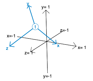
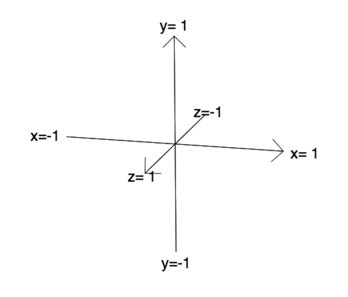
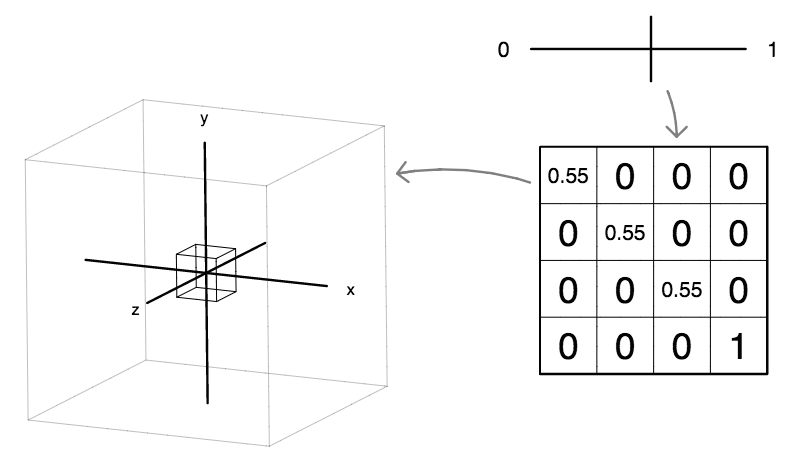
Coordinate transformations The default coordinate system in three dimensions has coordinate axes [1,0,0,0], [0,1,0,0] and [0,0,1,0], respectively (the x, y and z global direction vectors). Its origin is [0,0,0,1] (the point (0,0,0)), as shown in the figure to the right in black. We can describe a transformed coordinate system by redefining each of the x, y and z axes, and by translating the origin to point t, as shown in the figure to the right in blue. Note that this is a very general representation. For example, the new x, y and z directions do not need to be perpendicular to each other. Nor do they need to be unit length. For

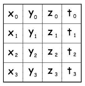
Transformation matrices All of the information of a coordinate transformation can be placed in a 4×4 matrix, as shown in the figure to the right. The x, y and z axes form the first three respective columns of the matrix. The origin t forms the right-most column of the matrix. In this class we will follow the convention of storing the 16 matrix values in column-major order: [ x0, x1, x2, x3,   y0, y1, y2, y3,   z0, z1, z2, z3,   t0, t1, t2, t3 ]

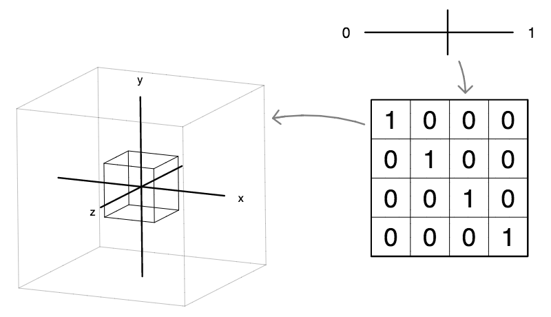
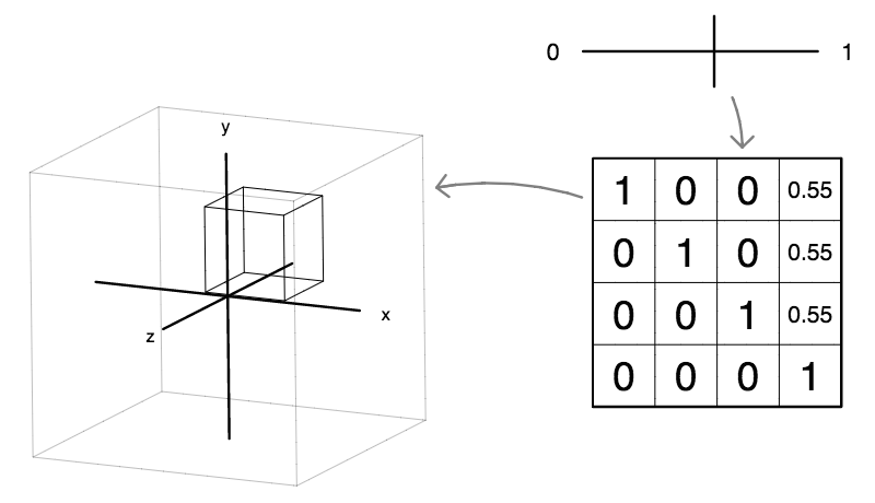
Transforming a point We can use a 4×4 matrix to transform a vector. By convention, we represent the input as a column vector, and place it to the right of the matrix. Also, by convention, if we omit the fourth (homogeneous) coordinate of the input, as in the example to the right, we assume a value of 1.0 for its homogeneous coordinate, unless otherwise specified. The result of the transformation is another column vector, which we obtain by taking the inner product of each successive row of the matrix with the input vector. In this case, the matrix is rotating the point (1,0,0) about the z axis.

The identity transformation The identity matrix is the "do nothing" transformation. It will transform any point or direction to itself. You generally want to call the identity() method on a matrix object to initialize that matrix.

The translate transformation To translate a point, we use only the right-most column of the matrix. The rest of the matrix is the same as the identity matrix. 1 0 0 Tx 0 1 0 Ty 0 0 1 Tz 0 0 0 1 Note that translation affects only points, not directions. Because the homogeneous coordinate of a direction is zero, its value cannot be affected by the right-most column of the matrix.

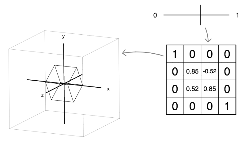
Rotate about the x axis Rotation about the x axis only affects the y and z axes. 1 0 0 0 0 cosθ -sinθ 0 0 sinθ cosθ 0 0 0 0 1 "Positive" rotation is counterclockwise when looking from the positive x direction.

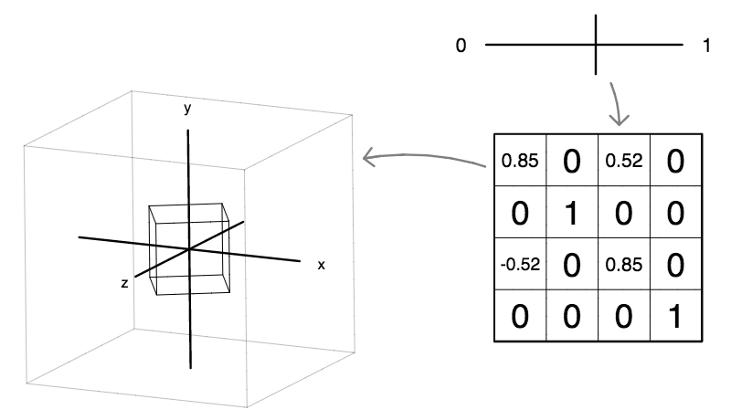
Rotate about the y axis Rotation about the y axis only affects the z and x axes. cosθ 0 sinθ 0 0 1 0 0 -sinθ 0 cosθ 0 0 0 0 1 "Positive" rotation is counterclockwise when looking from the positive y direction.

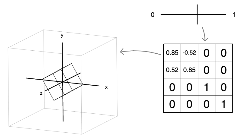
Rotate about the z axis Rotation about the z axis only affects the x and y axes. cosθ -sinθ 0 0 sinθ cosθ 0 0 0 0 1 0 0 0 0 1 "Positive" rotation is counterclockwise when looking from the positive z direction.

The scale transformation Like rotation, a scale transformation (which makes shapes bigger or smaller) uses only the top-left 3×3 portion of the 4#215;4 matrix. Sx 0 0 0 0 Sy 0 0 0 0 Sz 0 0 0 0 1 In the case illustrated on the right, we are performing a uniform scale, by using the same values for the three locations along the diagonal of the matrix. If we were to use differing values at these three locations, then we would perform a non-uniform scale, which would result in the shape becoming squashed or stretched.

The perspective transformation For completeness, we include the perspective transformation, although this is rarely used, except for setting up camera views. Note that the perspective transformation uses only the bottom row of the matrix. 1 0 0 0 0 1 0 0 0 0 1 0 Px Py Pz 1 Because perspective can change the homogeneous coordinate of an [x,y,z,w] vector, it is able to throw points out to infinity (that is, transform a point into a direction vector), as well as bring points at infinity into the scene (that is, transform a direction vector into a point).

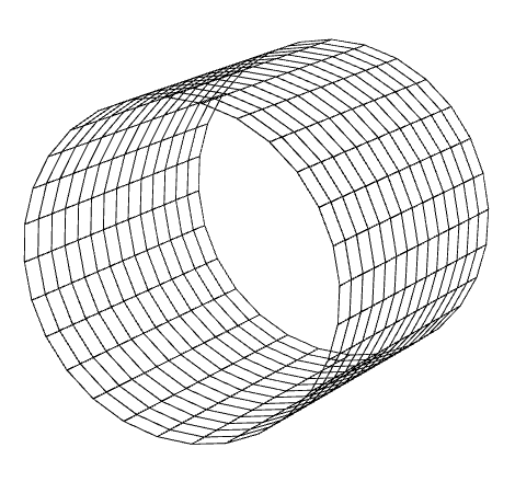
Parametric cylindrical tube Here is the core of a function that would return the x,y,z coordinates of a parametric cylindrical tube. Note that there are no caps at the end, so this is not a complete parametric cylinder. return [ cos(2*PI*u), sin(2*PI*u), 2*v-1 ];

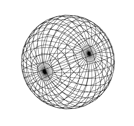
Parametric sphere Here is the core of a function that would return the x,y,z coordinates of a parametric sphere. Note that latitude φ varies between -π / 2 and π / 2. var theta = 2 * PI * u; var phi = PI * (v - .5) return [ cos(theta) * cos(phi), sin(theta) * cos(phi), sin(phi) ];

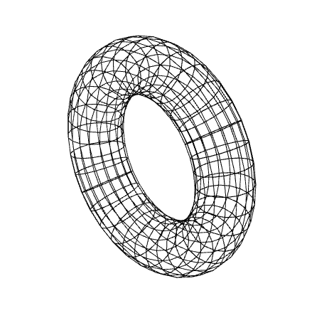
Here is the core of a function that would return the x,y,z coordinates of a parametric torus. Note that unlike the parametric sphere, φ varies between 0 and 2π. Parametric torus var theta = 2 * PI * u; var phi = 2 * PI * v; var r = 0.3; return [ cos(theta) * (1 + r * cos(phi)), sin(theta) * (1 + r * cos(phi)), r * sin(phi) ];

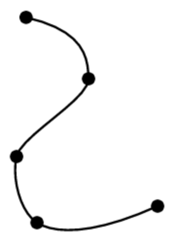
Splines There are many reasons we might want to create smooth controllable curves in computer graphics. Perhaps we might want to create an organic shape, or animate something along a continuous path. As you can see on the right, we can do this by breaking down our smooth curve into simpler pieces. If we think of the spline curve as a path of motion, each of these pieces must match its neighbors in both position and rate, which means that for each coordinate x and y, we need four values: a position at both the start and the end, and a rate (or derivative) at both the start and the end. The smallest order polynomial that can satisfy four constraints is a cubic. So we describe both the x and y coordinates of each piece using parametric cubic polynomials in parameter t: x = axt3 + bxt2 + cxt + dx y = ayt3 + byt2 + cyt + dy where (ax, bx, cx, dx) and (ay, by, cy, dy) are constant valued polynomial coefficients, and t varies from t = 0 to t = 1 along the curve.

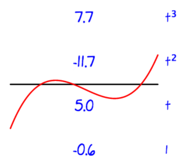
Cubic splines Although it is technically true that cubic splines can be designed by tweaking their polynial coefficients, in practice that doesn't usually work out very well. As you can see in the example on the right, there is no intuitive connection between the shape of a cubic polynomial and the values of its four coefficients -- in this case 7.7, -11.7, 5.0 and -0.6, respectively, for the t3, t2, t and constant term. For that reason, we need a better way to specify cubic spline curves. Rather than use t3, t2, t and 1 as our four basis functions, we can use four different basis functions that have a more intuitive geometric meaning. In the following sections we will look at different examples of such alternate basis functions.

Hermite cubic splines We can choose four basis functions that give us independent control over the position at t = 0 and t = 1, as well as the rate of change at t = 0 and t = 1. This is called the Hermite basis, after the french mathematician who devised it. If we want a curve with position A at t = 0, position B at t = 1, rate C at t = 0, and rate D at t = 1, we can use the four functions to the right to compute the cubic polynomial we are looking for. 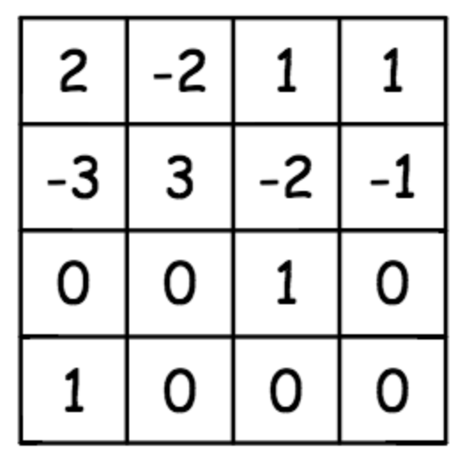Because these four hermite basis polynomials never change, and the cubic polynomial we want is just a weighted sum of those four polynomials, we can express this weighted sum as a multiplication of the weights by a matrix, which we call the Hermite matrix. In other words, the expression: A (2t3 - 3t2 + 1) + B (-2t3 + 3t2) + C (t3 - 3t2 + t) + D (t3 - t2) can be expressed as a matrix vector product: a b c d = A B C D to convert positions and rates at the two ends into the desired cubic polynomial: at3 + bt2 + ct + d.		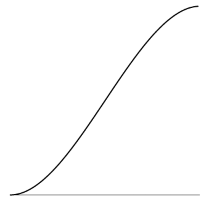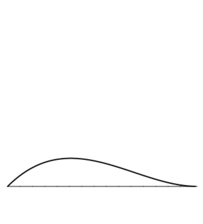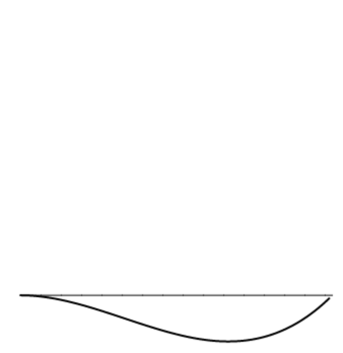Position 2t3 - 3t2 + 1 -2t3 + 3t2	Rate t3 - 2t2 + t t3 - t2

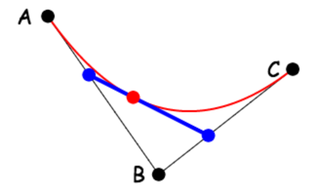
Bezier cubic splines Artists and designers often find it more convenient to create splines by moving points around, rather than needing to deal with derivatives. The Bezier spline enables designers of spline curves to work this way. Bezier splines work by repeated linear interpolation. For example, the image to the right shows a simplified version of a Bezier spline, using three key points to specify a parametric quadratic spline. Note that points along the curve are found as a linear interpolation of linear interpolations. We first find points along the edges AB and BC by linear interpolations (to get the points represented as blue dots): (1-t) A + t B (1-t) B + t C and then we interpolate again (to get the point represented as a red dot): P = (1-t) ( (1-t) A + t B ) + t ( (1-t) B + t C ) If we multiply out all the terms, we get: A (1-t)2 + 2 B (1-t) t + C t2 Note that the weights of the coefficients (1 2 1) follow Pascal's triangle:   1 1 1 1 2 1 1 3 3 1 ...
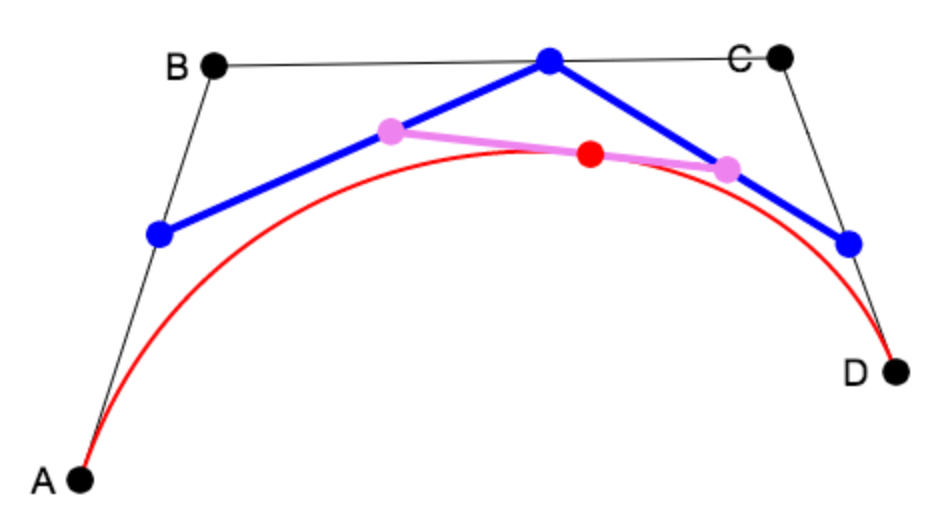
Now that we have looked at the quadratic case, we are ready to look at the cubic case. The parametric cubic Bezier spline uses four key points: The basic set-up is a linear interpololation of linear interpolations of linear interpolations. So we start with the points in blue: P = (1-t) A + t B Q = (1-t) B + t C R = (1-t) C + t D When the first and second terms are linearly interpolated, we get the two dots in violet: S = (1-t) P + t Q T = (1-t) Q + t R Finally we linearly interpolate these two points: (1-t) S + t T When we multiply everything out, writing the equation in terms of our original four key points A,B,C and D, the weights form the next level (1 3 3 1) of Pascal's triangle: A (1-t)3 + 3 B (1-t)2 t + 3 C (1-t) t2 + D t3
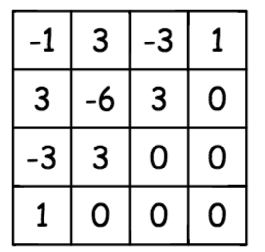
We can multiply out the terms of the above polynomial, and regroup by powers of t, to get: (-A + 3B - 3C + D) t3 + (3A - 6B + 3C) t2 + (-3A + 3B) t + A This makes it easy to see that, as was the case for Hermite splines, the Bezier spline has a characteristic matrix, which can be used to translate the above polynomial until the standard cubic polynomial, with coefficients (a,b,c,d): a b c d = A B C D One powerful property of Bezier splines is that the direction between A and B determines the direction of the spline curve at t=0, and the direction between C and D determines the direction of the spline curve at t=1. This makes it easy to match up splines end-to-end, so that the resulting composite curve has a continuous derivative.