For this week, I'd like you to use a combination of boolean intersection and first/second order surfaces to make a more geometrically interesting scene. For example, your scene can contain cylinders (intersection of a tube intersected with two half-spaces), some sort of polyhedron (intersection of half-spaces), or a flying saucer (intersection of two spheres).

In general, you will probably find that there is a tension between trying to do something that runs in "real time" and producing an amazingly gorgeously high quality rendered image. It's ok to focus on just one of these goals, rather than trying to optimize for both.

I'm also including a few extra topics, which some of you might want to try for extra credit.

If I get specific requests from any of you on any of the topics on this page, I'll put more detailed notes and suggestions about those topics. If you have some other specific ray-tracing related topic you want to pursue, let me know and I'll put up notes about that.

Better substrate

As we discussed in class, instead of using BufferedApplet, it is more efficient to write directly to the color framebuffer as an array. The Java library provides a way to do this through its Memory Image Source facility. To get started with this better way of doing things, download the source from the example I showed in class: http://mrl.nyu.edu/~perlin/MIS

Sub-sampling and super-sampling

You can choose to sub-sample at a lower effective resolution: For example, rather than shooting a ray at every pixel, you can shoot one every 3×3 pixels, or every 4×4 pixels, etc.

The general approach is to start out by sub-sample very n×nth pixel, and then go back and look at where there were large differences in color between two samples (in addition, you can also look for differences in distance or whether the adjoining rays have different surfaces). In those places where you find such differences (ie: at visual edges) go back and shoot a ray at every pixel.

You can also choose to super-sample at visual edges: rather than shoot only a single ray at pixels where you detect a large change in color from one pixel to the next, you can shoot 2×2 rays at those pixels, or 3×3 rays, etc. If you do this, then you should offset the aim directions of these rays so that each ray goes through a different part of the pixel. Then you can average the results from these n×<>n rays to get a smoothed or anti-aliased edge.

Ray tracing to generalized second order polynomials

In general you can describe any second order equation in three dimensions (an equation whose terms have polynomial powers of at most two) by ten terms:

ax² + by² + cz² + dyz + ezx + fxy + gx + hy + iz + j = 0

In order to ray trace to such surfaces, you would need to substitute [v_x+tw_x, v_y+tw_y, v_z+tw_z] into this equation, which will give you a quadratic equation only in t, which you could then solve.

One interesting question is: once you have found where the ray intersects such a surface, how do you compute the surface normal vector for shading? The answer is that you need to look at the derivative equation, which gives a vector valued gradient at each point:

[ 2ax + ez + fy + g , 2by + dz + fx + h , 2cz + dy + ex + i ]

Boolean union, intersection and difference

As we discussed in class, you can do boolean unions, intersections and differences along each ray to create composite objects.

The trick to developing a general boolean object is to maintain a list of "hits" of the ray with surfaces that it encounters, which should always remain sorted in order of increasing t. You then need to be able to combine those lists with union, intersection and difference operators.

Here is a slightly more robust version of the technique I described in class. Instead of relying on even/odd order (what I said in class), the version I describe here explicitly labels each hit as either being an "in" or an "out" hit. This will make your life easier when implementing the intersection algorithm.

Each item on a hit list should contain the following data fields: [t, surfaceId, sign = +1 or -1]. Their respective meanings are as follows:

• The t field is the parametric distance along the ray where the intersection occurred.

• The surfaceId is a unique identifier for the surface being intersected.

• The sign should be +1 if the ray is entering the object, or -1 if the ray is leaving the object.

To intersect two objects along a ray, you need to build an output list by using two indices to march along both input lists together:

• Starting at the beginning of both input lists, proceed at each step by incrementing the index of whichever hit comes next (ie: has the lower value of t):
  • If this hit is an "in", at a t value that is "in" on the other list, then append it as an "in" on your output list.

  • If this hit is an "out", at a t value that is "in" on the other list, then append it as an "out" on your output list.

I leave it up to you to figure out how to implement union (OR), intersection (AND) and difference (-) operators. One helpful hint: to implement the logical negation (¬) operator you just need to invert all the sign fields. With that observation, you only need to implement intersection. Then you can use the boolean equivalences:

A OR B = ¬ ( ¬A AND ¬B )
A - B = A AND ¬B

Ray tracing to polyhedra

First, let's define a half-space (a,b,c,d) by its characteristic equation ax+by+cz+d≤0. In other words, this half-space consists of those points (x,y,z) such that ax+by+cz+d≤0. Notice that the half-space is bounded by the plane ax+by+cz+d=0.

Here's a simple observation: If you can ray trace to a plane, then you can ray trace to any convex polyhedron, since a convex polyhedron can be defined as an intersection of half-spaces.

For example, here are the coefficients of the six half-spaces that define a unit cube:

a	b	c	d
-1	0	0	-1
1	0	0	-1
0	-1	0	-1
0	1	0	-1
0	0	-1	-1
0	0	1	-1

a(v_x+tw_x) + b(v_y+tw_y) + c(v_z+tw_z) + d ≤ 0

To intersect the ray with the entire polyhedron, just intersect the ray with each of its constituent half-spaces, and can call your ∧ operator on all the results.

When it comes time to do shading, you'll need a normal vector. As always, you can obtain this by taking the vector-valued derivative, or "gradient", of the half-space's characteristic equation. To do this, you take the three partial derivatives, in x, y and z, respectively, of ax+by+cz+d. These are, respectively, a, b and c. Therefore, the gradient is just the constant vector [a,b,c]. If you normalize this vector to unit length you obtain the surface normal vector.

Shadows

We already discussed this somewhat last week, but I will review here. Once your ray has hit that first visible surface point, which we can refer to as s = (s_x,s_y,s_z), the key is to create another ray that goes from s into the direction of the light vector L, and see whether that ray intersects anything.

If this shadow ray hits anything, then the surface point is in shadow, and should only be illuminated by the ambient color. If the shadow ray doesn't hit anything, then the surface point should be fully illuminated by that light source.

When you shoot this ray, one danger is that your ray tracer will accidentally find the surface point s itself, due to numerical inaccuracies. You don't want that. To avoid this, the trick that I usually employ is to use, as the origin of the shadow ray, not exactly s itself, but a point that's already been moved a little bit along the ray by some small distance ε. So your ray should actually be defined by v+tw, where: v = s+εL and w = L (the direction toward the light source).

Transparency and refraction

One topic we did not discuss in class, but which you might want to try for extra credit, is refraction.

In addition to a ray of light bouncing off a surface, some of the light might actually go through the surface. This can happen, for example, if light encounters such transparent materials as glass or water or lucite. When this happens in nature, there is generally refraction, or bending of light where the ray enters or leaves the transparent material.

Refraction is governed by Snell's Law, which states that light will bend in a way that is determined by the material's index of refraction, or n, which indicates how much more slowly the light travels in this medium, in comparison with the speed of light in a vacuum. For example, light travels through a material with an index of refraction of n=1.5 at a speed of 1/1.5, or 2/3 of the speed of light in a vacuum.

The speed of light through air is so close to the speed of light in a vacuum that we can pretty much approximate its index of refraction by n=1. The index of refraction of glass is typically around n=1.4.

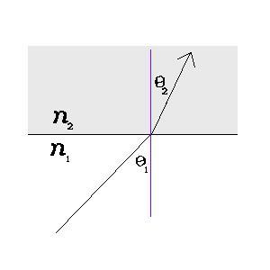
Specifically, Snell's Law states that if an incoming ray travelling through a medium that has an index of refraction of n₁ crosses over into another medium that has an index of refraction of n₂, then the relationship between the angle θ₁ by which the entering ray deviates from the surface normal, and the angle θ₂ by which the exiting ray deviates from the surface normal, is given by n₁ sinθ₁ = n₂ sinθ₂ .

Atmosphere: fog, pea soup, etc.

Another topic we did not discuss in class, but which is very easy to implement and can make your ray traced scenes look a lot cooler, is atmosphere. You can opt to add this for extra credit if you have time.

In the presence of fog, objects gradually fade from view, as a function of their distance from your eye. In the case of uniform fog (ie: fog with the same density everywhere), it is pretty easy to model and render this effect. The key observation is that for any uniform fog there is some distance D that a beam light has to travel before half of the light in the beam has been scattered away by fog particles. The other half of the light continues along the beam unobstructed.

Now consider what happens when the light which has made it through the fog travels further by another distance D. Half of the remaining light will now be scattered away, and half of the remaining light will make it through the second distance. In other words, the light that makes it through a distance 2D unobstructed is (1/2)². And in general, the amount of light that makes it through a distance kD is (1/2)^k, for any value of k.

To calculate uniform fog which scatters half of its light every distance D, you need to measure the distance d traveled by the ray (ie: the distance from the ray origin to the surface point that the ray hits). The proportion of this light that makes it through the fog unscattered will be t=(1/2)^d/D. The effect of the fog can be shown by mixing t(surfaceColor) + (1-t)(fogColor), where surfaceColor is the color that you would have calculated had there been no fog. Some uniform shade of light gray, such as (0.8,0.8,0.8), generally works well for the fog color.

How to transform a general quadratic equation in three dimensions

As I pointed out in class, plane equation ax + by + cz + d, which characterizes the plane p containing points x^T, can be defined by the following dot product:

(a b c d)

•

x y z 1

=   0

or, in other words, p x^T = 0. This makes it clear that if you want to find the plane that contains transformed points M•x^T, then you need to replace p with p M^-1.

Similarly, we can define quadratic equation

ax² + by² + cz² + dyz + ezx + fxy + gx + hy + iz + j = 0

(x,y,z,1)

•

a f e g 0 b d h 0 0 c i 0 0 0 j

•

x y z 1

=   0

or in other words, x P x^T = 0, where P denotes the 10 quadratic coefficients arranged into the above 4×4 matrix.

This means that if you want to find the three-variable quadratic equation that contains transformed points M•x^T, you need to replace P by (M^-1)^T P M^-1, because that will give you:

(M x^T)^T     (M^-1)^T P M^-1     (M x^T)     =
x^T M^T     (M^-1)^T P M^-1     M x^T     =
x P x^T = 0

NEW MATERIAL ADDED TO THE NOTES:

In case you were not able to either implement or find on-line a MatrixInverter algorithm, here is one you can use.

Also, one thing that might not be obvious, is that when you create the product of

(M^-1)^T P M^-1

   x*x x*y x*z x*1
   y*x y*y y*z y*1
   z*x z*y z*z z*1
   1*x 1*y 1*z 1*1

This will leave you with just the ten unique coefficients of the quadratic in three variables, in the upper right of your transformed matrix.

With the above machinery, you can define simple second order surfaces, for which [a,b,c,d,e,f,g,h,i,j] are easy to define, such as a unit sphere: [1,1,1,0,0,0,0,0,0,-1], or a unit radius cylindrical tube along the z axis: [1,1,0,0,0,0,0,0,0,-1], and animate them by 4×4 matrices.

Homework, due before class on Thursday April 12

Your homework this week is to make a cool animated ray traced scene that contains more interesting shapes than just spheres.

You will need to implement ray tracing to transformed first order surfaces and to transformed second order surfaces. That means applying the same matrices you have been using all semester to the transform math I've described in the last section of these notes.

At the very least, create shapes that are the result of convex intersections, such as cylinders and cubes. This will allow you to use the simple intersection trick we discussed in class: taking the maximum of all "in" hits, and the minimum of all "out" hits.

For extra credit, implement the more general intersection algorithm that handles non-convex shapes. This will allow you to create far more interesting things.

For extra credit, implement refraction, atmospheric effects, sub-sampling for speed, and super-sampling for antialiasing.