Homework 5, due Tuesday, Nov 2

This is the second ray tracing assignment. In this assignment I'm going to ask you to:

• Incorporate the Phong shading model;
• Ray trace to polyhedra;
• Ray trace to general second order surfaces (such as cylinders and cones);
• Do simple boolean intersections of convex shapes.

In the notes that accompany this assignment will be all the material you need to do these things.

There is also an extra credit topic at the end if you're feeling really ambitious.

The Phong shading model:

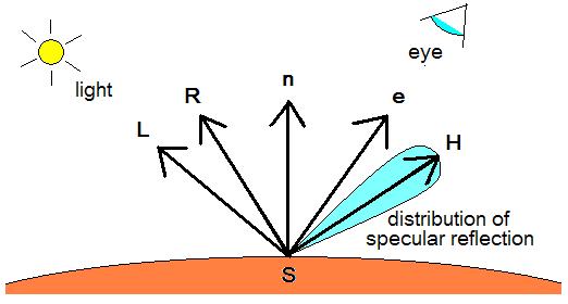
The Phong surface shding model is described by:

Ambient_color + SUM_i ( LightColor_i   *   ( Diffuse_color * max(0,L_i•n) + Specular_color * (max(0,H_i•e)^p ) )

For each light source the corresponding highlight direction vector H_i (the direction toward the mirror reflection of the light source), is computed by H_i = 2(L_i • n) n - L_i

Generally speaking, a surface looks like plastic if is has white specular highlights, regardless of its diffuse or ambient color. A surface looks more like colored metal (such as copper, brass or gold) when its highlight color has the same r,g,b mix as its diffuse and ambient colors (although the highlight can be brighter).

For now you can just assume that the lights are all positioned essentially at infinity, so that all the rays of light from each light source will be parallel (like the Sun, for example). Practically, this means that you can just use a single direction vector for any one light source.

Note that each light source is described by both its r,g,b color, and its x,y,z direction. So you need a total of six numbers to describe one light source.

You can also try to implement shadows, which really are not that hard to do with ray tracing. The trick is, when you're at a single surface point and looping over light sources, fire a ray from the surface point into the direction of each light source. If the ray hits any geometry, then don't illuminate that surface point by that light source (ie: don't add in any Diffuse or Specular contributions for that light source).

Ray tracing to polyhedra:

As we said in class, to implement ray tracing to polyhedra:

• Describe the polyhedron as an intersection of half-spaces, where each half-space is a linear inequality (a,b,c,d), such that a point (x,y,z) is on the inside of the face when ax+by+cz+d <= 0. Note that the surface normal for any point on this face is in the direction of the gradient vector (a,b,c).

  For example, the six linear inequalities for a unit cube are:

  				a	b	c	d
  x > -1	→	-x-1 < 0	→	-1	0	0	-1
  x < +1	→	+x-1 < 0	→	+1	0	0	-1
  y > -1	→	-y-1 < 0	→	0	-1	0	-1
  y < +1	→	+y-1 < 0	→	0	+1	0	-1
  z > -1	→	-z-1 < 0	→	0	0	-1	-1
  z < +1	→	+z-1 < 0	→	0	0	+1	-1

• Ray trace to any planar face by substituting (v_x+tw_x, v_y+tw_y, v_z+tw_z) for (x,y,z), and then solving for t = 0.

  If the planar face is facing toward the camera (ie: if v is on the positive-valued outside of the face), then t is at a point where the ray enters the polyhedron.

  Conversely, if the planar face is facing away from the camera (ie: if v is on the negative-valued inside of the face), then t is at a point where the ray exits the polyhedron.

• The place where the ray enters the polyhedron is the maximum among all the entering t values.

• The place where the ray exits the polyhedron is the minimum among all the exiting t values.

• If the entering t is less than the exiting t, then the ray has indeed struck the polyedron. Otherwise, the ray has missed the polyhedron.

• The surface normal where the ray enters the polyhedron is obtained from the (a,b,c) coefficients of the plane at which the ray entered the polydron (ie: of the entering plane that had the maximum value of t).

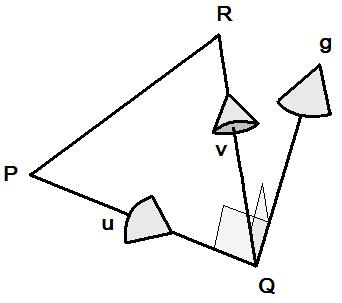
You can figure out the linear inequality (a,b,c,d) that goes through the face of any polygon, by considering any three of the polygon's vertices P,Q,R. Remember that we are following the convention that the point P,Q,R go around counterclockwise, as seen from the outside (ie: from the positive-valued half-space) of the shape. The method is as follows:

Take the difference vectors u = Q - P and v = R - Q. Take their cross product g = u × v, where cross product is defined by ( uyvz - uzvy , uzvx - uxvz , uxvy - uyvx ). Vector g gives the direction into which the gradient function increases the fastest. So you can use the components of g as your a,b,c coefficients. Also, if you normalize g to unit length, you get the surface normal n. You then just need to choose the fourth coefficient d such that one of your polygon vertices, say Q, lies on plane defined by ax+by+cz+d=0. In other words: gxPx + gyPy + gzPz + d = 0, so you can just set d = -g•Q.

Transforming polyhedral shapes:

In the discussion that follows, I'm going use transpose notation (x y z 1)^T when referring to the homogeneous decription of a point in space, to make it clear that I am describing the point as a column vector.

When transforming a half-space (a b c d) by matrix M, the key thing to observe is that if you transform each point

(x y z 1)^T → M(x y z 1)^T,

then your corresponding transformation (a b c d) → (a' b' c' d') has to ensure that the transformed point still lies on the same side of the transformed plane:

(a' b' c' d') (M(x y z 1)^T) = (a b c d) (x y z 1)^T.

In other words, if we ask the question "is this point inside the original half-space?", we need to get the same answer after we transform both the point and the half-space.

As we discussed in class, the way to do this is to post-multiply by the matrix inverse, so that:

(a b c d) → ( (a b c d) M^-1 ).

This works because linear transformations are associative:

( (a b c d) M^-1 )   ( M(x y z 1)^T ) =
(a b c d)   ( M^-1 M )   (x y z 1)^T =
(a b c d)   I   (x y z 1)^T =
(a b c d) (x y z 1)^T

Ray tracing to second order polynomial shapes:

A second order polynomial shape is defined by a second order polynomial. That's a polynomial where the sum of the powers of any term is not greater than two. Examples are x² + y² - 1 and xy + 3.

In contrast, a polynomial like x²z + y² - 1 is not second order, because the sum of the powers in the first term x²z is too high: 2 + 1 = 3.

The most general possible second order polynomial has ten terms:

ax² + by² + cz² + dxy + eyz + fzx + gx + hy + iz + j

For points at the surface, you can compute the x,y,z partials of the gradient direction (the direction which points perpendicularly out of the surface). If you normalize this gradient vector to unit length, you get the surface normal.

As you probably know from your freshman calculus class, you can get the x,y,z components of this gradient vector by taking the derivative of the polynomial with respect to x,y and z, respectively:

( 2ax+dy+fz+g , 2by+dx+ez+h , 2cz+ey+fx+i )

If you want to transform a second order polynomial by a linear transformation matrix, it is useful to describe the evaluation of the polynomial at any point (x y z 1)^T by using the notation of linear transformations. As we discussed in class, the following notation, devised by Jim Blinn, does the trick, by forming the polynomial coefficients into a 4×4 matrix:

The above expression multiplies out to exactly ax² + by² + cz² + dxy + eyz + fzx + gx + hy + iz + j.

Now that we have the equation in this form, we can transform the original point and see what happens. First we transform (x y z 1)^T to (M (x y z 1)^T). We also need to transform the point in the other place it appears - on the left side of the coefficients matrix. When you transpose vectors and matrices, you end up reversing the order that they multiply together, so (x y z 1) is transformed to ((x y z 1) M^T).

Following the same logic that we used for transforming half-spaces, we need to insert a matrix both to the left and to the right of the coefficients matrix, so that the result of the transformed equation doesn't change:

As we discussed in class, we do this as follows:

Of the three terms above, the middle term gives the transformed coefficients matrix. In order to compute this, you will need to be able to invert a 4×4 matrix. For convenience I am providing you with a matrix inverter.

Boolean intersections:

Given a collection of convex shapes, if the ray misses any one of them, then the ray misses their intersection. If the ray hits all of them, then the intersection is given by the interval [max(t_in) , min(t_out)], where max(t_in) is the maximum over all the t_in, and where min(t_in) is the minimum over all the t_out.

For example, you can create a unit length cylinder by intersecting the infinite cylinder x² + y² - 1 = 0 with the cube that goes from -1 to +1 in x, y and z. Then you can apply a matrix to the component shapes in order to transform this cylinder to any other finite length cylinder.

Boolean unions and differences (making non-convex shapes):

Non-convex shapes are more difficult to deal with than are convex shapes, because the same ray can enter and leave a shape multiple times, to it is not sufficient just to speak of a single interval [t_in , t_out]. Instead, we need to describe the places where the ray is inside the shape by a sequence of t values: [ t₀ t₁ t₂ ... t_n-1 ], where the even numbered elements represent places where the ray enters the shape, and the odd numbered elements represent places where the ray exits from the shape. For example, [0.3   1.4   2.7   3.5] represents two successive segments where the ray is inside the shape: a first segment between t=0.3 and t=1.4, followed by a second segment between t=2.7 and t=3.5.

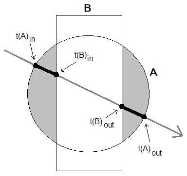
This notation makes it possible to describe non-convex things like the result of boolean difference. For example, suppose shape A contains a hollow cavity with shape B, and suppose that a particular ray intersects shape A at [t(A)in , t(A)out], and that the same ray intersects shape B at [t(B)in , t(B)out]. If t(A)in <   t(B)in <   t(B)out <   t(A)in, then the boolean difference A - B is described along this ray by: [ t(A)in   t(B)in   t(B)out   t(A)out ].

In general you can implement boolean difference by replacing:

[ t₀   t₂   t₃ ... t_n-1 ]   →   [ 0   t₀   t₁   t₂ ... t_n-1   ∞ ]

Notice that if t₀ was already zero, then the first interval becomes null, and you can just drop the first two elements of the resulting sequence. Similarly, if if t_n-1 was already ∞ then you can just drop the last two elements of the resulting sequence.

In order to implement boolean union, you only need to implement boolean intersection and boolean difference, since de Morgan's law gives us:

A ˇ B = ¬ ( (A ˆ B) ˆ (A ˆ B) )

The hardest part is implementing intersection for non-convex shapes. To intersect two non-convex shapes along a ray you need to merge together their two sequences. This is done by progressively moving along the two sequences, looking for values of t where the ray is inside both shapes, and using those values of t to construct a new sequence. Here is a sketch of the algorithm:

   Create an empty destination sequence.

   Starting from the beginning of both sequences,
   Repeat until at the end of both sequences:

      Choose the smallest remaining t value, from whichever of the
      two input sequences you find it.

      If this was an entering (even numbered) t:
         If this t value is inside the other shape:
            then append it to the destination sequence.

      If this was an exiting (odd numbered) t:
         If this t value is outside the other shape:
            then append it to the destination sequence.

Your job for this assignment is to come up with an interesting collection of tinted reflecting and shaded shapes, and use the above code and equations to ray trace to them, to produce a cool and compelling picture or animation. Try to use a variety of shapes.