If you recall, we showed in class that the way to evaluate bicubic spline patch surfaces is to treat the X(u,v), Y(u,v) and Z(u,v) coordinates independently, and to proceed as follows for each of them. To create the coefficients matrix for X(u,v), you use the characteristic basis matrix M for that type of spline to transform the 4×4 values of your geometry matrix G into 4×4 values of a coefficients matrix Cx:
C = M • Gx • MTIf you recall, the code that I used to do this for my planet example looks something like:
   constructBicubicCoefficients(double[][] G, double[][] M, double[][] C) {
      double[][] tmp = new double[4][4];

      for (int i = 0 ; i < 4 ; i++)    // tmp = G • MT
      for (int j = 0 ; j < 4 ; j++)
      for (int k = 0 ; k < 4 ; k++)
	 tmp[i][j] += G[i][k] * M[j][k];

      for (int i = 0 ; i < 4 ; i++)    // C = M • tmp
      for (int j = 0 ; j < 4 ; j++)
      for (int k = 0 ; k < 4 ; k++)
	 C[i][j] += M[i][k] * tmp[k][j];
   }
Once you've constructed the coefficients matrix, then you can evaluate the X coordinate of the spline surface by:
X(u,v) = [v3 v2 v 1] • Cx • [u3 u2 u 1]TIn my planet example, I did this with code that looks something like:
   double evalBicubic(double C[][], double u, double v) {
      return u * (u * (u * (v * (v * (v * C[0][0] + C[0][1]) + C[0][2]) + C[0][3])
                         + (v * (v * (v * C[1][0] + C[1][1]) + C[1][2]) + C[1][3]))
                         + (v * (v * (v * C[2][0] + C[2][1]) + C[2][2]) + C[2][3]))
                         + (v * (v * (v * C[3][0] + C[3][1]) + C[3][2]) + C[3][3]);
   }
You would construct and evaluate Y(u,v) and Z(u,v)
in exactly the same way,
starting with appropriate values for
Gy and
Gz.
In all your Bezier spline work, you used the Bezier basis:
   double[][] M_Bez = {             // Bezier basis matrix
      {-1, 3,-3, 1},
      { 3,-6, 3, 0},
      {-3, 3, 0, 0},
      { 1, 0, 0, 0}
   };
Just so you have it, here are the bases
matrices for some other interesting splines...
In my planet example, I used the Catmull-Rom basis, which interpolates through all the control points:
   double[][] M_C_R = {             // Catmull-Rom basis matrix
      {-0.5,  1.5, -1.5, 0.5},
      { 1  , -2.5,  2  ,-0.5},
      {-0.5,  0  ,  0.5, 0  },
      { 0  ,  1  ,  0  , 0  }
   };
When your input is in the form of values and gradients
at the four corners of your patch surface,
then you would use the Hermite basis:
   double[][] M_H   = {             // Hermite basis matrix
      { 2,-2, 1, 1},
      {-3, 3,-2,-1},
      { 0, 0, 1, 0},
      { 1, 0, 0, 0}
   };
When you want to make a
non-interpolating spline, which is
influenced by control points but does
not actually go through them, then you use
the uniform B-spline basis:
   double[][] M_B = {               // B-spline basis matrix
      {-1/6., 1/2.,-1/2., 1/6.},
      { 1/2.,-1.  , 1/2., 0   },
      {-1/2., 0   , 1/2., 0   },
      { 1/6., 2/3., 1/6., 0   }
   };
Your basic assignment this week is to make a shape which is modeled as a set of bicubic patches that fit together seamlessly. I'd like you to render this shape into your zbuffer renderer. Render the individual bicubic patch surfaces by using the same polygonal meshes that you are already using, but create each of those meshes by constructing and evaluating a bicubic spline patch.
For example, you might have a 16×16 polygon mesh as your basic rendered primitive, and you might construct this mesh by specifying a Bezier patch, and then sampling that patch at regular intervals:
   double meshVertices[][][] = new double[17][17][6];

   for (int iu = 0 ; iu <= 16 ; iu++)
   for (int iv = 0 ; iv <= 16 ; iv++) {
      double u = iu / 16.;
      double v = iv / 16.;
      meshVertices[iu][iv][0] = evalBicubic(C_x, u, v);
      meshVertices[iu][iv][1] = evalBicubic(C_y, u, v);
      meshVertices[iu][iv][2] = evalBicubic(C_z, u, v);
   }
and then creating a set of 16×16 four-sided polygonal faces to connect these vertices.
One interesting question is how to handle the normals at each vertex. You certainly want the normals at the edges and corners of neighboring patches to be the same. I can suggest two different ways you might do this. Both of them work just fine:
evalBicubic,
and implement corresponding methods
evalBicubicPartialU and
evalBicubicPartialV
to compute the partial derivatives in
u and v.
For any given value of
u and v,
the x,y,z coordinates of these partials form
two tangent vectors
du[3] and
dv[3] on the patch surface at that point.
The surface normal is just the cross product
of these two vectors (which you'll then want to normalize of course).
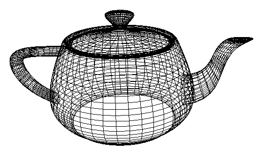
I would like you to apply your code to the following teapot shape, which is actually the famous Newell Teapot, the first really interesting shape that was ever described as a set of Bezier patches. It has a fascinating history, which you might want to read about here.

The set of 32 Bezier control patches defining this teapot is given here. You can declare this data as an array in your applet. Note that the data for the 16 respective control points of each patch is ordered: x0,y0,z0, x1,y1,z1, ... x15,y15,z15.
As usual, feel free to go wild with cool design or challenging technical innovations for extra credit. For example, you might want to distort the shape of your teapot in interesting ways, or try to generate other interesting shapes that are defined as patches. You might want to create an interesting terrain surface, perhaps using my Noise function, using a basis such as Catmull-Rom or B-spline to define the control points. Or you can try to procedurally generate hairlike surfaces, or a creature with billowing wings that flex over time.
Giving the user interesting opportunities to interact with your model is always highly encouraged.