Start Lecture #1
I start at 0 so that when we get to chapter 1, the numbering will agree with the text.
There is a web site for the course. You can find it from my home page, which is http://cs.nyu.edu/~gottlieb
Start Lecture #1marker above can be thought of as
after lecture #0.
The course text is Dale, Joyce, and Weems,
Object-Oriented Data Structures Using Java
.
It is available at the NYU Bookstore.
Replyto contribute to the current thread, but NOT to start another topic.
top post, that is, when replying, I ask that you either place your reply after the original text or interspersed with it.
musttop post.
Grades are based on the labs, the midterm, and the final exam, with each very important. The weighting will be approximately 30%*Labs, 30%*Midterm, and 40%*Final (but see homeworks below).
I use the upper left board for lab/homework assignments and announcements. I should never erase that board. Viewed as a file it is group readable (the group is those in the room), appendable by just me, and (re-)writable by no one. If you see me start to erase an announcement, let me know.
I try very hard to remember to write all announcements on the upper left board and I am normally successful. If, during class, you see that I have forgotten to record something, please let me know. HOWEVER, if I forgot and no one reminds me, the assignment has still been given.
I make a distinction between homeworks and labs.
Labs are
Homeworks are
Homeworks are numbered by the class in which they are assigned. So any homework given today is homework #1. Even if I do not give homework today, the homework assigned next class will be homework #2. Unless I explicitly state otherwise, all homeworks assignments can be found in the class notes. So the homework present in the notes for lecture #n is homework #n (even if I inadvertently forgot to write it to the upper left board).
I feel it is important for majors to be familiar with basic
client-server computing (nowadays sometimes called
cloud computing
in which one develops on a client machine (for
us, most likely your personal laptop), but run programs on a remote
server (for us, most likely i5.nyu.edu).
You submit the jobs from the server and your final product remains
on the server (so that we can check dates in case we lose you
lab).
I have supposedly given you each an account on i5.nyu.edu. To access i5 is different for different client (laptop) operating systems.
You may develop lab assignments on any system you wish, but ...
I sent it ... I never received itdebate. Thank you.
The following is supposed to work; let's see.
  mailx -s "the subject goes here" gottlieb@nyu.edu
  words go here and go in the msg.
  The next line causes a file to be placed in the msg (not attached
  simply copied in)
  ~r filename
  .
Good methods for obtaining help include
You labs must be written in Java.
Incomplete
The rules for incompletes and grade changes are set by the school and not the department or individual faculty member.
The rules set by CAS can be found here. They state:
The grade of I (Incomplete) is a temporary grade that indicates that the student has, for good reason, not completed all of the course work but that there is the possibility that the student will eventually pass the course when all of the requirements have been completed. A student must ask the instructor for a grade of I, present documented evidence of illness or the equivalent, and clarify the remaining course requirements with the instructor.
The incomplete grade is not awarded automatically. It is not used when there is no possibility that the student will eventually pass the course. If the course work is not completed after the statutory time for making up incompletes has elapsed, the temporary grade of I shall become an F and will be computed in the student's grade point average.
All work missed in the fall term must be made up by the end of the following spring term. All work missed in the spring term or in a summer session must be made up by the end of the following fall term. Students who are out of attendance in the semester following the one in which the course was taken have one year to complete the work. Students should contact the College Advising Center for an Extension of Incomplete Form, which must be approved by the instructor. Extensions of these time limits are rarely granted.
Once a final (i.e., non-incomplete) grade has been submitted by the instructor and recorded on the transcript, the final grade cannot be changed by turning in additional course work.
This email from the assistant director, describes the departmental policy.
  Dear faculty,

  The vast majority of our students comply with the
  department's academic integrity policies; see

  www.cs.nyu.edu/web/Academic/Undergrad/academic_integrity.html
  www.cs.nyu.edu/web/Academic/Graduate/academic_integrity.html

  Unfortunately, every semester we discover incidents in
  which students copy programming assignments from those of
  other students, making minor modifications so that the
  submitted programs are extremely similar but not identical.

  To help in identifying inappropriate similarities, we
  suggest that you and your TAs consider using Moss, a
  system that automatically determines similarities between
  programs in several languages, including C, C++, and Java.
  For more information about Moss, see:

  http://theory.stanford.edu/~aiken/moss/

  Feel free to tell your students in advance that you will be
  using this software or any other system.  And please emphasize,
  preferably in class, the importance of academic integrity.

  Rosemary Amico
  Assistant Director, Computer Science
  Courant Institute of Mathematical Sciences
The university-wide policy is described here
You should have taken 101 (or if not should have experience in Java programming).
A goal of this course is to improve your Java skills. We will not be learning many new aspects of Java. Instead, we will be gaining additional experience with those parts of Java taught in 101.
The primary goal of this course is to learn several important data structures and to analyze how well they perform. I do not assume any prior knowledge of this important topic.
A secondary goal is to learn and practice a little client-server computing. My section of 101 did this, but I do not assume you know anything about it.
In 101 our goal was to learn how to write correct programs in Java.
Step 1 in that goal, the main step in 101, was to learn how to write anything in Java.
We did consider a few problems (e.g., sorting) that required some thought to determine a solution, independent of the programming language, but mostly we worried about how to do it in Java.
In this course we will go beyond getting a correct program and seek programs that are also high performance, i.e., that have comparatively short running time even for large problems.
One question will be how to measure the performance.
Of course we can not sacrifice correctness for performance, but sometimes we will sacrifice simplicity for performance.
public class Max {
  public int max(int n, int[]a) {
    // assumes n > 0
    int ans = a[0];
    for (int i=0; i<n; i++)
      if (a[i] > ans)
    ans = a[i];
    return ans;
  }
}
Assume you have N numbers and want to find the kth largest. If k=1 this is simply the minimum; If k=N this is simply the maximum; If k=N/2 this is essentially the median.
To do maximum you would loop over N numbers as shown on the right. Minimum is the same simple idea.
Both of these are essentially optimal: To find the max, we surely need to examine each number so the work done will be proportional to N and the program above is proportional to N.
Homework: Write a Java method that computes the 2nd largest. Hint calculate both the largest and 2nd largest; return the latter.
The median is not so simple to do optimally. One method is fairly obvious and works for any k: Read the elements into an array; sort the array; select the desired element.
It might seem silly to sort all N elements since we don't care about the order of all those past the median. So we could do the following.
This second method also works for any k.
Both these methods are correct (the most important criterion) and simple. The trouble is that neither method has optimal performance. For large N, say 10,000,000 and k near N/2, both methods take a long time; whereas a more complicated algorithm is very fast.
Another example is given in section 5.3 where we choose a circular array implementation for queues rather than a simpler array implementation because the former is faster.
In 101, we had objects of various kinds, but basically whenever we
had a great deal of data, it was organized as an array (of
something).
An array is an example of a data structure
.
As the course title suggests, we will learn a number of other data
structures this semester.
Sometimes these data structures will be more complicated than simpler ones you might think of. Their compensating advantage is that they have higher performance.
Also we will learn techniques useful for large programs. Although we will not write any large programs, such programs are crucially important in practice. For example, we will use Java generics and interfaces to help specify the behavior we need to implement.
Client-server systems (now often referred to as
cloud computing
are of increasing importance.
The idea is that you work on your client computer with assistance
from other server systems.
We will do some of this.
In particular, we will use the computer i5.nyu.edu as a server.
We need to confirm that everyone has an account on i5.nyu.edu.
Homework: As mentioned previously, those of you with Windows clients, need to get putty and winSCP. They are definitely available on the web at no cost. (The last time I checked, winSCP available through ITS and putty was at http://bit.ly/hy9IZj).
I will do a demo of this software next class. Please do install it by then so you can verify that it works for you.
macOS users should see how to have their terminal run in plain (ascii) text mode.
Read.
Read.
Read.
We have covered this in 101, but these authors tie the attributes of object orientation to the goals of quality software just mentioned.
Read
This section is mostly a quick review of concepts we covered in 101. In particular, we covered.
Most of you learned Java from Liang's book, but any Java text should be fine. Another possibility is my online class notes from 101.
The book does not make clear that the rules given are for data fields and methods. Visibility modifiers can also be used on classes, but the usage and rules are different.
I have had difficulty deciding how much to present about visibility. The full story is complicated and more than we need, but I don't want to simplify it to the extent of borderline inaccuracy. I will state all the possibilities, but describe only those that I think we will use.
A .java file consists of 1 or
more classes.
These classes are called top level
since they are not inside
any other classes.
Inside a class we can define methods, (nested) classes, and fields The later are often called data fields and sometimes called variables. I prefer to reserve the name variables for those declared inside methods.
class TopLevel1 {
  public    int   pubField;
  private   int   pvtField;
  protected int   proField;
            int   defField;
  public    class PubNestedClass {}
  private   class PriNestedClass {}
  protected class ProNestedClass {}
            class DefNestedClass {}
}
public class TopLevel2 {
  public    static void main (String[] arg) {}
  private   static void pvtMethod() {}
  protected static void proMethod() {}
            static void defMethod() {}
}
Top-level classes have two possible visibilities: public and package-private (the default when no visibility keyword is used). Each .java file must contain exactly one top-level public class, which corresponds to the name of the file
Methods, fields, and nested classes each have four possible visibilities: public, private, protected, and package-private (the default).
The two visibilities for top-level classes, plus the four visibilities for each of the three other possibilities give a total of 14 possible visibilities, all of which are illustrated on the right.
Question: What is the filename?
For now we will simplify the situation and write .java files as shown on the right.
// one package statement
// import statements
public class NameOfClass {
  // private fields and
  // public methods
}
An object is an instantiation of a class. Each object contains a copy of every instance (i.e., non-static) field in the class. Conceptually, each object also contains a copy of every instance method. (Some optimizations do occur to reduce the number of copies, but we will not be concerned with that.)
In contrast all the objects instantiated from the same class share class (i.e., static) fields and methods.
public class ReferenceVsValueSemantics {
  public static void main (String[] args) {
    int a1 = 1;   C c1 = new C(1);
    int a2 = 1;   C c2 = new C(1);
    a1 = a2;      c1 = c2;
    a1 = 5;       c1.setX(5);
    System.out.println(a2 + " " + c2.getX());
  }
}

public class C {
  private int x;
  C (int x) { this.x = x; }
  public int  getX()      { return x; }
  public void setX(int x) { this.x = x; }
}

javac ReferenceVsValueSemantics.java C.java
java  ReferenceVsValueSemantics
This is a huge deal in Java. It is needed to understand the behavior of objects and arrays. Unfortunately it can seem a little strange at first. Consider the program on the right, which is composed of two .java files.
Below the source files are the two commands I used to compile and run the program.
I formatted the main method to show that the a's and the c's are treated similarly.
Let's review this small example carefully as it illustrates a number of issues.
You should be absolutely sure you understand why the two values printed are not the same.
Start Lecture #2
Remark: If your last name begins with A-K your grader is Arunav Borthakur; L-Z have Prasad Kapde. This determines to whom you email your lab assignments
Remark: Chen has kindly created a wiki page on using WinSCP and Putty. See https://wikis.nyu.edu/display/~xc402/How+to+connect+to+NYU+i5+server.
Lab: Lab 1 parts 1 and 2 are assigned and are due 13 September 2012. Explain in class what is required.
In all Java systems, you run a program by invoking the
Java Virtual Machine
(aka JVM).
The primitive method to do this, which is the only one I use, is to
execute a program named java.
The argument to java is the name of the class file (without the .class extension) containing the main method. A class file is produced from a Java source file by the Java compiler javac. Each .java file is often called a compilation unit since each one is compiled separately.
If you are using an Integrated Development Environment
(IDE), you probably click on some buttons somewhere, but the result
is the same: The Java compiler javac is given each .java
file as a compilation unit and produces class files; the JVM
program java is run on the class file containing the main
method.
Inheritance was well covered in 101; here I add just a few comments.
  public class D extends B {
    ...
  }
biggerthan B objects.
biggerthan the set of C objects
Java (unlike C++) permits only what is called
single inheritance
.
That is, although a parent can have several children, a child can
have just one parent (a biologist would call this asexual
reproduction).
Single inheritance is simpler than multiple inheritance.
For one thing, single inheritance implies that the classes form a
tree, i.e., a strict hierarchy.
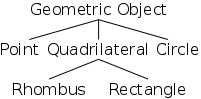
For example, on the right we see a hierarchy of geometric concepts.
Note that a point is a
geometric object and a rhombus
is a
quadrilateral.
Indeed, for every line in the diagram, the lower concept is a
upper concept.
This so-called ISA relation suggests that the lower concept should
be a class derived from the upper.
Indeed the handout shows classes with exactly these inheritances. The Java programs can be found here.
You might think that Java classes form a forest not a tree since you can write classes that are not derived from any other. One example would be ReferenceVsValueSemantics above. However, this belief is mistaken. Any class definition that does not contain the extends keyword, actually extends the built-in class object. Thus Java classes do indeed form a tree, with object as the root.
(I reordered the material in this section.)
Java permits grouping a number of classes together to for a package, which gives the following advantages.
package packageName;
The syntax of the package statement is trivial as shown on the right. The only detail is that this statement must be the first (nonblank, noncomment) line in the file.
  import packageName.ClassName;
  import packageName.*
To access the contents of another package, you must either
import java.util.Scanner;
public class Test {
  public static void main(String[] arg) {
    int x;
    Scanner getInput = new Scanner(System.in);
    x = getInput.nextInt();
  }

public class Test {
  public static void main(String[] arg) {
    int x;
    java.util.Scanner getInput =
             new java.util.Scanner(System.in);
    x = getInput.nextInt();
  }
}
For example, recall from 101 the important Scanner class used to read free-form input. This class is found in the package java.util.
To read an int, one creates a Scanner object (I normally call mine getInput) and then invokes the nextInt() method in this object.
The two examples on the right illustrate the first and third procedures mentioned above for accessing a package's contents. (For the second procedure, simply change java.util.Scanner to java.util.*.
Note that both the Scanner class and the nextInt() method have public visibility. How do I know this and where can you go to check up on me?
The key is to go to java.sun.com. This will send you to an Oracle site, but Java is a Sun product; Oracle simply bought Sun. You want Java SE-->documentation-->API
Let's check and see if I was right that Scanner and nextInt() are public.
Homework: How many methods are included in the Scanner class? How many of them are public?
The name of a package constrains where its files are placed in the filesystem. First, assume a package called packageName consisting of just one file ClassName.java (this file defines the public class ClassName). Although not strictly necessary, we will place this .java files in a directory called packageName.
javac packageName/ClassName.java
To compile this file we go to the parent directory of packageName and type the command on the right. (I use the Unix notation, / for directories; Windows uses \.)
Unlike the situation above, most packages have multiple .java files.
javac packageName/*.java
If the package packageName contains many .java files, we place them all in a directory also called packageName and compile them by going to the parent of packageName and executing the command on the right.
Just as the .java files for a package named packageName go in a directory named packageName, the .java files for a package named first.second go in the subdirectory second of a directory named first.
javac first/second/*.java
To compile these .java files, go to the parent of first and type the command on the right
javac first/second/third*.java
Similarly a package named first.second.third would be compiled by the command on the right.
The simplest situation is to leave the generated .class flies in the same directory as the corresponding .java files and execute the java command from the same directory that you executed the javac command, i.e., the parent directory.
I show several examples on the right.
  java packageName/ClassName

  java testPackage/Test

  java bigPackage/M

  java first/second/third/M
The examples above assume that there is just one package, we keep the .class files in the source directory, and we only include classes from the Java library. All of these restrictions can be dropped by using the CLASSPATH environment variable.
  public class Test {
    public static void main (String[] args) {
      C c = new C();
      c.x = 1;
    }
  }

  public class C {
    public int x;
  }
The basic question is
Where do the compiler and JVM look for .java
and .class files?
.
First consider the 2-file program on the right. You can actually compile this with a simple javac Test.java. How does the compiler find the definition of the class C?
The answer is that it looks in all .java files in the current directory. We use CLASSPATH if we want the compiler to look somewhere else.
Next consider the familiar line
include java.util.Scanner;
.
How does the compiler (and the JVM) find the definition of
the Scanner class?
Clearly java.util is a big clue, but where do they look
for java.util.
The answer is that they look in the system jar file
(whatever that is).
We use CLASSPATH if we want it to look somewhere else in
addition.
Many of the Java files used in the book are available on the web (see page 28 of the text for instructions on downloading). I copied the directory tree to /a/dale-datastructures/bookFiles on my laptop.
In the subdirectory ch02/stringLogs we find all the .java files for the package ch02.stringLogs.
One of these files is named LLStringNode.java and contains the definition of the corresponding class. Hopefully the name signifies that this class defines a node for a linked list of strings.
import ch02.stringLogs.LLStringNode;
public class DemoCLASSPATH {
  public static void main (String[] args) {
    LLStringNode lLSN =
       new LLStringNode("Thank you CLASSPATH");
    System.out.println(lLSN.getInfo());
  }
}
I then went to directory java-progs not related to /a/dale-datastructures/bookFiles and wrote the simple program on the right.
A naive attempt to compile this with javac DemoCLASSPATH.java fails since it cannot find a the class LLStringNode in the subdirectory ch02/stringLogs (indeed java-progs has no such directory.
export CLASSPATH=/a/dale-datastructures/bookFiles:.
However once CLASSPATH was set correctly, the compilation succeeded. On my (gnu-linux) system the needed command is shown on the right.
Homework: 28. (When just a number is given it refers to the problems at the end of the chapter in the textbook.)
Data structures describe how data is organized.
Some structures give the physical organization, i.e., how the data is stored on the system. For example, is the next item on a list stored in the next higher address, or does the current item give the location explicitly, or is there some other way.
Other structures give the logical organization of the data. For example is the next item always larger than the current item? For another example, as you go through the items from the first, to the next, to the next, ..., to the last, are you accessing them in the order in which they were entered in the data structure?
Well studied in 101.
We will study linked implementations a great deal this semester. For now, we just comment on the simple diagram to the right.
groundsymbol from electrical engineering).
Start Lecture #3
Remark: Chen will have an office hour Wednesdays 5-6pm in CIWW 412.
For these structures, we don't describe how the items are stored, but instead which items can be directly accessed.
The defining characteristic of a stack is that you can access or remove only the remaining item that was most recently inserted. We say it has last-in, first-out (LIFO) semantics. A good real-world example is a stack of dishes, e.g., at the Hayden dining room.
In Java-speak
we say a stack object has three public
methods: top() (which returns the most recently inserted
item remaining on the list), pop() (which removes the
most recently inserted remaining item), and push() (which
inserts its argument on the top of the list).
Many authors define pop() to both return the top element and remove it from the stack. That is, many authors define pop() to be what we would call top();pop().
The defining characteristic of a queue is that you can remove only the remaining item that was least recently inserted. We say it has first-in, first-out (FIFO) semantics. A good example is an orderly line at the bank.
In java-speak, we have enqueue() (at the rear) and dequeue() (from the front). (We might also have accessors front(), and rear().
Homework: Customers at a bank with many tellers form a single queue. Customers at a supermarket with many cashiers form many queues. Which is better and why?
Here the first element is the smallest, each succeeding element is larger (or equal to) its predecessor, and hence the last element is the largest. It is also possible for the elements to be in the reverse order with the largest first and the smallest last.
One natural implementation of a sorted list is an array with the elements in order; another is a linked list, again with the elements in order. We shall learn other structures for sorted lists, some of which provide searching performance much higher than either an array or simple linked list.
The structures we have discussed are one dimensional (except for higher-dimensional arrays). Each element except the first has a unique predecessor, each except the last has a unique successor, and every element can be reached by starting at one end and heading toward the other.
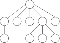
Trees, for example the one on the right, are different. There is no single successor; pictures of trees invariable are drawn in two dimensions, not just one.
Note that there is exactly one path between any two nodes.
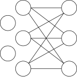
Trees are a special case of graphs. In the latter, we drop the requirement of exactly one path between any two nodes. Some nodes may be disconnected from each other and others may have multiple paths between them.
A specific method for organization, either logically or physically.
A references is a pointer to (or the address of) an object; they are typically drawn as arrows.
public class ReferenceVsValueSemantics {
  public static void main (String[] args) {
    int a1 = 1;   C c1 = new C(1);
    int a2 = 1;   C c2 = new C(1);
    a1 = a2;      c1 = c2;
    a1 = 5;       c1.setX(5);
    System.out.println(a2 + " " + c2.getX());
  }
}

public class C {
  private int x;
  C (int X) { this.x = x; }
  public int  getX()      { return x; }
  public void setX(int x) { this.x = x; }
}

javac ReferenceVsValueSemantics.java C.java
java  ReferenceVsValueSemantics
We covered this topic is section 1.3, but it is such a huge deal in Java that we will cover it again here (using the same example). Reference semantics determine the behavior of objects and arrays. Unfortunately these semantics can seem a little strange at first. Consider the program on the right, which is composed of two .java files.
Below the source files are the two commands I used to compile and run the program.
I formatted the main method to show that the a's and the c's are treated similarly.
Let's review this small example carefully as it illustrates a number of issues.
You should be absolutely sure you understand why the two values printed are not the same.
Continuing with the last example, we note that c1 and c2 refer to the same object. They are sometimes called aliases. As the example illustrated, aliases can be confusing; it is good to avoid them if possible.
What about the top ellipse (i.e., object) in the previous diagram for which there is no longer a reference? Since it cannot be named, it is just wasted space that the programmer cannot reclaim. The technical term is that the object is garbage. However, there is no need for programmer action or worry, the JVM detects garbage and collects it automatically.
The technical terminology is that Java has a built-in garbage collector.
Thus Java, like most modern programming languages supports the run-time allocation and deallocation of memory space, the former is via new, the latter is performed automatically. We say that Java has dynamic memory management.
  // Same class C as above
  public class Example {
    public static void main (String[] args) {
      C c1 = new C(1);
      C c2 = new C(2);
      C c3 = c1;
      for (int i=0; i<1000; i++) {
        c3 = c2;
        c3 = c1;
      }
    }
  }
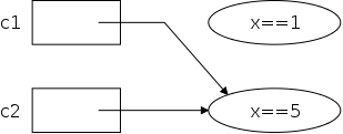
Execute the code on the right in class. Note that there are two objects (one with x==1 and one with x==2) and three references (the ones in c1, c2, and c3).
As execution proceeds the number of references to the object with x==1 changes from 1 to 2 to 1 to 2 ... . The same pattern occurs for the references to the other object.
Homework: Can you
write a program where the number of references to a fixed object
changes from 1 to 2 to 3 to 2 to 3 to 2 to 3 ... ?
Can you write a program where the number of references to a fixed
object changes from 1 to 0 to 1 to 0 to 1 ... ?
In Java, when you write r1==r2, where the r's are variables referring to objects, the references are compared, not the contents of the objects. Thus r1==r2 evaluates to true if and only if r1 and r2 are aliases.
We have seen equals() methods in 101 (and will see them again this semester). Some equals() methods, such as the one in the String class, do compare the contents of the referred to objects. Others, for example the one in the object class, act like == and compare the references.
First we need some, unfortunately not standardized, terminology. Assume in your algebra class the teacher defined a function f(x)=x+5 and then invoked it via f(12). What would she call x and what would she call 12. As mentioned above, usage differs.
I call x (the item in the callee's definition) a parameter and I call 12 (the item in the caller's invocation) an argument. I believe our text does as well.
Others refer to the item in the callee as the
formal parameter
and the item in the caller as the
actual parameter
.
Still others use argument
and parameter
interchangeably.
After settling on terminology, we need to understand Java's parameter passing semantics. Java always uses call-by-value semantics. This means.
public class DemoCBV {
  public static void main (String[] args) {
    int x = 1;
    CBV cBV = new CBV(1);
    System.out.printf("x=%d  cBV.x=%d\n", x, cBV.x);
    setXToTen(x, cBV);
    System.out.printf("x=%d  cBV.x=%d\n", x, cBV.x);
  }
  public static void setXToTen(int x, CBV cBV) {
    x = 10;   cBV.x = 10;
  }
}
public class CBV {
  public int x;
  public CBV (int x) {
    this.x = x;
  }
}
Be careful when the argument is a reference. Call-by-value still applies to the reference but don't mistakenly apply it to the object referred to. For example, be sure you understand the example on the right.
Well covered in 101.
There is nothing new to say: an array of objects is an array of
objects.
You must remember that arrays are references and objects are
references, so there can be two layers of arrows
.
Also remember that you will need a new to create the
array and another new to create each
object.
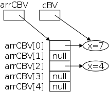
The diagram on the right shows the result of executing
  cBV = new CBV(7);
  CBV[] arrCBV = new CBV[5];
  arrCBV[0] = cBV;
  arrCBV[2] = new CBV(4);
Note that only two of the five array slots have references to objects; the other three are null.
Lab: Lab 1 part 3 is assigned and is due in 7 days.
As discussed in 101, Java does not, strictly speaking, have 2-dimensional arrays (or 3D, etc). It has only 1D arrays. However each entry in an array can itself be an array
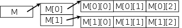
On the right we see a two dimensional array M with two rows and three columns that can be produced by executing
  int[][] M;
  M = new int [2][3];
Note that M, as well as each M[i] is a reference. The latter are references to int's; whereas, the former is a reference to an array of int's.
2d-arrays such as M above in which all rows have the same length are often called matrices or rectangular arrays and are quite important.
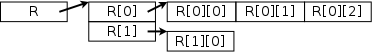
Java however does support so-called ragged arrays
such as
R shown on the right.
That example can be produced by executing
  int [][] R;
  R = new int [2][];
  R[0] = new int [3];
  R[1] = new int [1];
Homework: Write a Java program that creates a 400 by 500 matrix with entry i,j equal to i*j.
The idea is to approximate the time required to execute an algorithm (or a program implementing the algorithm) independent of the computer language (or the compiler / computer). Most importantly we want to understand how this time grows as the problem size grows.
For example, suppose you had an unordered list of N names and wanted to search for a name that happens not to be on the list.
You would have to test each of the names. Without knowing more, it is not possible to give the exact time required. It could be 3N+4 seconds or 15n+300 milliseconds, or many other possibilities.
But it cannot be 22 seconds or even 22log(N) seconds. You just can't do it that fast (for large N).
If we look at a specific algorithm, say the obvious check one entry at a time, we can see the time is not 5N2+2N+5 milliseconds. It isn't that slow (for large N).
Indeed that obvious algorithm takes AN+B seconds, we just don't know A and B.
We will crudely approximate the above analysis by saying the algorithm has (time) complexity (or takes time) O(N).
That last statement is really sloppy. We just did three analyses. First we found that the complexity was greater than 22log(N), and then we found that the complexity was less than 5N2+2N+5, and finally we asserted the complexity was AN+B. The big-Oh notation strictly speaking covers only the second (upper-bound) analysis; but is often used, e.g., by the authors, to cover all three.
The rest of this optional section is from a previous incarnation of 102, using a text by Weiss.
We want to capture the concept of comparing function growth where
we ignore additive and multiplicative constants.
For example we want to consider 4N2-500N+1 to
be equivalent
to 50N2+1000N and want to
consider either of them to be bigger than
1000N1.5log(N).
Definition: A function T() is said to be big-Oh of f() if there exists constants c and n0 such that T(N)≤cf(N) whenever N≥n0. We write T=O(f).
Definition: A function T() is said to be big-Omega of f() if f=O(T). We write T=Ω(f).
Definition: A function T() is said to be Theta of f() if T=O(f) and T=Ω(f). We write T=Θ(f).
Definition: A function T() is said to be little-Oh of f() if T=O(f) but T≠Θ(f). We write T=o(f).
Definition: A function T() is said to be little-Omega of f() if f=o(T). We write T=ω(f).
It is difficult to decide how much to emphasize algorithmic analysis, a rather mathematical subject. On the one hand
On the other hand
As a compromise, we will cover it, but only lightly (as does our text).
For the last few years we used a different text, with a more mathematical treatment. I have left that material at the end of these notes, but, naturally, it is not an official part of this semester's courses.
As mentioned above we will be using the big-O
(or big-Oh
) notation to indicate we are giving an
approximation valid for large N.
(I should mention that the O above is really the Greek Omicron.)
We will be claiming that, if N is large (enough), 9N30 is insignificant when compared to 2N.
Most calculators cannot handle really large numbers, which makes the above hard to demo.
import java.math.BigInteger;
public class DemoBigInteger {
  public static void main (String[] args) {
    System.out.println(
      new BigInteger("5").multiply(
         new BigInteger("2").pow(1000)));
  }
}
Fortunately the Java library has a class BigInteger that allows arbitrarily large integers, but it is a little awkward to use. To print the exact result for 5*21000 you would write a program something like the one shown on the right.
To spare you the anxiety of wondering what is the actual answer, here it is (I added the line breaks manually).
  53575430359313366047421252453000090528070240585276680372187519418517552556246806
  12465991894078479290637973364587765734125935726428461570217992288787349287401967
  28388741211549271053730253118557093897709107652323749179097063369938377958277197
  30385314572855982388432710838302149158263121934186028340346880
Even more fortunately, my text editor has a built in infinite precision calculator so we can try out various examples. Note that ^ is used for exponentiation, B for logarithm (to any base), and the operator is placed after the operands, not in between.
Do the above example using emacs calc.
The following functions are ordered from smaller to larger
N-3 N-1 N-1/2 N0 N1/3 N1/2 N1 N3/2 N2 N3 ... N10 ... N100Three questions that remain (among many others) are
To answer the first question we will (somewhat informally) divide one function by the next. If the quotient tends to zero when N gets large, the second is significantly larger that the first. If the quotient tends to infinity when N gets large, the second is significantly smaller than the first.
Hence in the above list of powers of N, each entry is significantly larger than the preceding. Indeed, any change in exponent is significant.
The answer to the second question is that log(N) comes after N0 and before NP for every fixed positive P. We have not proved this.
The answer to the third question is that 2N comes after NP for every fixed P. (The 2 is not special. For every fixed Q>1, QN comes after every fixed NP.) Again, we have not proved this.
Do some examples on the board.
Read. The idea is to consider two methods to add 1+2+3+4+...+N
These have different big-Oh values.
So a better algorithm has better (i.e., smaller) complexity.
Imagine first that you want to calculate (0.3)100. The obvious solution requires 99 operations.
In general for a fixed b≠0, raising bN using the natural algorithm requires N-1=O(N) operations.
I describe the algorithm for the special case of .3100 but it works in general for bN. The basic idea is to write 100 in binary and only use those powers. On the right is an illustration.
  1    2    4    8   16   32   64  128


  0    0    1    0    0    1    1   0


 .3   .32  .34  .38  .316 .332 .364


           .32     ×     .332 × .364
Since there were just 4 large steps, each of which has complexity O(log(N)), so does the entire algorithm.
Homework: The example above used N=100. The natural algorithm would do 99 multiplications, the better algorithm does 8. Assume N≤1,000,000. What is the maximum number of multiplications that the natural algorithm would perform? What is the maximum number of multiplications that the better algorithm would perform?
Start Lecture #4
Assume the phone book has N entries.
If you are lucky, the first entry succeeds, this takes O(1) time.
If you are unlucky, you need the last entry or, even worse, no entry works. This takes O(N) time.
Assuming the entry is there, on average it will be in the middle. This also takes O(N) time.
From a big-Oh viewpoint, the best case is much better than the average, but the worst case is the same as the average.
Lab: Lab 1 part 4 is assigned and is due in 7 days.
The above is kinda-sorta OK. When we do binary search for real will get the details right. In particular we will worry about the case where the sought for item is not present.
This algorithm is a big improvement. The best case is still O(1), but the worst and average cases are O(log(N)).
BUT binary search requires that the list is sorted. So either we need to learn how to sort (and figure out its complexity) or learn how to add items to a sorted list while keeping it sorted (and figure out how much this costs.
This are not trivial questions; we will devote real effort on their solutions.
Read
  public class Quadrilateral extends GeometricObject {
    ...
    public Quadrilateral (Point p1, Point p2,
                          Point p3, Point P4)
    public double area() {...}
  }
Definition: An Abstract Data Type is a data type whose properties are specified but not their implementations. For example, we know from the abstract specification on the right that a Quadrilateral is a Geometric Object, that it is determined by 4 points, and that its area can be determined with no additional information.
The idea is that the implementor of a modules does not reveal all the details to the user. This has advantages for both sides.
In 201 you will learn how integers are stored on modern computers (twos compliment), how they were stored on the CDC 6600 (ones complement), and perhaps packed decimal (one of the ways they are stored on IBM mainframes). For many applications, however, the implementations are unimportant. All that is needed is that the values are mathematical integers.
For any of the implementations, 3*7=21, x+(y+z)=(x+y)+z (ignoring overflows), etc. That is, to write many integer-based programs we need just the logical properties of integers and not their implementation. Separating the properties from the implementation is called data abstraction.
Consider the BigDecimal class in the Java library that we mentioned previously (it includes unbounded integers). There are three perspectives or levels at which we can study this library.
Preconditions are requirements placed on the user of a method in order to ensure that the method behaves properly. A precondition for ordinary integer divide is that the divisor is not zero.
A postcondition is a requirement on the implementation. If the preconditions are satisfied, then upon method return the postcondition will be satisfied.
This is Java's way of specifying an ADT. An interface is a class with two important restrictions.
The implied keywords public static final and public abstract can be (and typically are) omitted.
A method without a body is specified at the user level, it tells you what arguments you must supply and the type of the value returned. It does not tell you how any properties of the return value or any side effects of the method (e.g., values printed).
Each interface used must be implemented by one or more real classes that have non-abstract versions of all the methods.
The next two sections give examples of interfaces and their implementing classes. You can also read the FigureGeometry interface in this section.
As a warm up for the book's Stringlog interface, I present an ADT and two implementations of the trivial operation of squaring an integer. I even threw in a package. All in all it is way overblown. The purpose of this section is to illustrates the Java concepts in an example where the actual substance is trivial and the concepts are essentially naked.
There are four .java files involved as shown on the right and listed below. The first three constitute the squaring package and are placed in a directory with the same name (standard for packages).
  package squaring;
  public interface SquaringInterface {
    int getSquare();
  }

  package squaring;
  public class SimpleSquaring implements SquaringInterface {
    private int x;
    public SimpleSquaring(int x)  { this.x = x; }
    public int getSquare()        { return x*x; }
  }

  package squaring;
  public class FancySquaring implements SquaringInterface {
    private int x;
    public FancySquaring(int x)  { this.x = x; }
    public int getSquare() {
      int y = x + 55;
      return (x+y)*(x-y)+(y*y);
    }
  }

  import squaring.*;
  public class DemoSquaring {
    public static void main(String[] args) {
      SquaringInterface x1 = new SimpleSquaring(5);
      SquaringInterface x2 = new FancySquaring(6);
      System.out.printf("(x1.x)*(x1.x)=%d (x2.x)(x2.x)=%d\n",
                        x1.getSquare(), x2.getSquare());
    }
  }
The first file is the ADT. The only operation supported is to compute and return the square of the integer field of the class. Note that the (non-constant) data field is not present in the ADT and the (abstract) operation has no body.
The second file is the natural implementation, the square is computed by multiplying. Included is a standard constructor to create the object and set the field.
The third file computes the square in a silly way (recall that (x+y)*(x-y)=x*x-y*y). The key point is that from a client's view, the two implementations are equivalent (ignoring performance).
The fourth file is probably the most interesting. It is located in the parent directory. Both variables have declared type SquaringInterface. However, they have actual types SimpleSquaring and FancySquaring respectively.
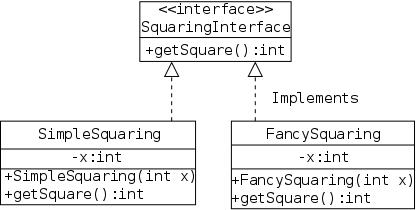
A Java interface is not a real class so no object can have actual type SquaringInterface (only a real class can follow new). Since the getSquare() in each real class overrides (not overloads) the one in the interface, the actual type is used to choose which one to invoke. Hence x1.getSquare() invokes the getSquare() in SimpleSquaring; whereas x2.getSquare() invokes the getSquare() is FancySquaring().
UML is a standardize way of summarizing
classes and
interfaces.
For example, the 3 classes/interfaces for in the squaring
package would be written as shown on the right.
The commands in this section are run from the parent directory of squaring. Note that the name of this parent is not important. What is important is that the name of the squaring must agree with the package name.
  javac squaring/*.java

  javac DemoSquaring.java
  java  DemoSquaring
It would be perfectly fine to execute the three lines on the right, first compiling the package and then compiling and running the demo.
However, the first line is not necessary. The import statement in DemoSquaring.java tells the compiler that all the classes in the squaring package are needed. As a result the compiler looks in subdirectory squaring and compiles all the classes.
Homework: 9, 10.
In contrast to the above, we now consider an example of a useful package.
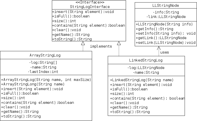
The book's stringLogs package gives the specification and two implementations of an ADT for keeping logs of strings. A log has two main operations, you can insert a string into the string and ask if a given string is already present in the log.
Homework: If you haven't already done so, download the book's programs onto your computer. It can be found at http://samples.jbpub.com/9781449613549/bookFiles.zip.
Unzip the file and you will have a directory hierarchy starting at XXX/bookFiles, where XXX is the absolute name (i.e. starting with / or \) of the directory at which you executed the unpack. Then set CLASSPATH via
As mention previously much of the book's code can be downloaded onto your system. In my case I put it in the directory /a/dale-dataStructures/bookFiles. Once again the name of this directory is not important, but the names of all subdirectories and files within must be kept as is to agree with the usage in the programs
  import ch02.stringLogs.*
  public class DemoStringLogs {
  }
To prepare for the serious work to follow I went to a scratch directory and compiled the trial stub for a stringLog demo shown on the right. The compilation failed complaining that there is no ch02 since DemoStringLogs.java is not in the parent directory of ch02.
Since I want to keep my code separate from the book's, I do not want my demo in /a/dale-dataStructures/BookFiles. Instead I need to set CLASSPATH.
export CLASSPATH=/a/dale-dataStructures/bookFiles:.
The command on the right is appropriate for my gnu/linux system and (I believe) would be the same on MacOS. Windows users should see the book. This will be demoed in the recitation.
Now javac DemoStringLogs.java compiles as expected.
StringLog(String name);
Since a user might have several logs in their program, it is useful for each log to have a name. So we will want a constructor something like that on the right.
For some implementations there is a maximum number of entries possible in the log. (We will give two implementations, one with and one without this limit.)
StringLog(String name, int maxEntries);
If we have a limit, we might want the user to specify its value with a constructor like the one on the right.
nicely formattedversion of the log.
Here is the code downloaded from the text web site. One goal of an interface is that a client who reads the interface can successfully use the package.
That is an ambitious goal; normally more documentation is needed.
How about the questions I raised in the previous section?
  import ch02.stringLogs.*;
  public class DemoStringLogs {
    public static void main (String[] args) {
      StringLogInterface demo1;
      demo1 = new ArrayStringLog ("Demo #1");
      demo1.insert("entry 1");
      demo1.insert("entry 1"); // ??
      System.out.println ("The contains() " +
        "method is case " +
        (demo1.contains("Entry 1") ? "in" : "")
        + "sensitive.");
      System.out.println(demo1);
    }
  }

  The contains() method is case insensitive.
  Log: Demo #1

  1. entry 1
  2. entry 1
On the right we have added some actual code to the demo stub above. As is often the case we used test cases to find out what the implementation actually does. In particular, by compiling (javac) and running (java) DemoStringLogs we learn.
conditional expression(borrowed from the C language).
nicely formattedoutput of the toString() method.
Homework: 15.
Homework: Recall that a stringlog can contain multiple copies of the same string. Describe another method that would be useful if multiple strings do exist.
Start Lecture #5
Now it is time to get to work and implement StringLog.
  package ch02.stringLogs;
  public class ArrayStringLog
         implements StringLogInterface {
    ...
  }
In this section we use a simple array based technique in which a StringLog is basically an array of strings. We call this class ArrayStringLog to emphasize that it is array based and to distinguish it from the linked-list-based implementation later in the chapter.
 private String[] log;
 private int lastIndex = -1;
 private String name;
Each StringLog object will contain the three instance fields on the right: log is the basic data structure, an array of strings with each array entry containing one log entry. name is the name of the log and lastIndex is is the last index (i.e., largest) into which an item has been placed.
The book uses protected (not private) visibility. For simplicity I will keep to the principal that fields are private and methods public until we need something else.
  public ArrayStringLog(String name,
                        int maxSize) {
    this.name = name;
    log = new String[maxSize];
  }

  public ArrayStringLog(String name) {
    super(name, 100); // 100 arbitrary
  }
We must have a constructor
Why?
That is, why isn't the default constructor adequate?
Answer: Look at the fields, we need to set name and
create the actual array.
Clearly the user must supply the name, the size of the array can either be user-supplied or set to a default. This gives rise to the two constructors on the right.
Although the constructor executes only two Java statements, its complexity is O(N) (not simply O(1). This is because each string in the array is automatically initialized to the empty string. You can see this if you read the String constructor.
Both constructors have the same name, but their signatures (name plus parameter types) are different so Java can distinguish them.
  public void insert (String s) {
    log[++lastIndex] = s;
  }
This mutator executes just one simple statement so is O(1). Inserting an element into the log is trivial because.
  public void clear() {
    for(int i=0; i<=lastIndex; i++)
      log(i) = null;
    lastIndex = -1;
  }
To empty a log we just need to reset lastIndex.
Why?
If so, why the loop?
  public boolean isFull() {
    return lastIndex == log.length-1;
  }

  public String size() {
    return lastIndex+1;
  }

  public String getName() {
    return name;
  }
The isFull() accessor is trivial (O(1)), but easy to get wrong by forgetting the -1. Just remember that in this implementation the index stored is the last one used not the next one to use and all arrays start at index 0.
For the same reason size() is lastIndex+1. It is also clearly O(1)
The accessor getName() illustrates why accessor methods
are sometimes called getters.
So that users cannot alter fields
behind the implementor's back
, the fields are normally
private and the implementor supplies a getter.
This practice essentially gives the user read-only access to the
fields.
  public boolean contains (String str) {
    for (int i=0; i<=lastIndex; i++)
      if (str.equalsIgnoreCase(log(i))
        return true;
    return false;
  }
The contains() method loops through the log looking for the given string. Fortunately, the String class includes an equalsIgnoreCase() so case insensitive searching is no extra effort.
Since the program loops through all N entries it must take time that grows with N. Also each execution of equalsIgnoreCase() can take time that grows with the length of the entry. So the complexity is more complicated and not just O(1) or O(N)
  public String toString() {
    String ans = "Log: " + name + "\n\n";
    for (int i=0; i<=lastIndex; i++)
      ans = ans + (i+1) + ". " + log[i] + "\n";
    return ans;
  }
The toString() accessor is easy but tedious.
It's specification is to return a nicely formatted
version of
the log.
We need to produce the name of the log and each of its entries.
Different programmers would often produce different programs since
what is nicely formatted
for one, might not be nicely
formatted for another.
The code on the right (essentially straight from the book) is
one reasonable implementation.
With such a simple implementation, the bugs should be few and shallow (i.e., easy to find). Also we see that the methods are all fast except for contains() and toString(). All in all it looks pretty good, but ...
Conclusion: We need to learn about linked lists.
Homework: 20, 21.
Read.
As noted in section 1.5, arrays are accessed via an index, a value that is not stored with the array. For a linked representation, each entry (except the last) contains a reference or pointer to the next entry. The last entry contains a special reference, null.
Before we can construct a linked version of a stringlog, we need to define a node, one of the horizontal boxes (composed of two squares) on the right.
The first square Data is application dependent.
For a stringlog, it would be a string, but in general it could be
arbitrarily complex.
However, it need not be arbitrarily complex.
Why?
The Next entry characterizes a linked list; it is a pointer to another node. Note that I am not saying one Node contains another Node, rather that one node contains a pointer to (or a reference to) another node.
As an analogy consider a treasure hunt
game where you are
given an initial clue, a location (e.g., on top of the basement TV).
At this location, you find another clue, ... , until the last clue
points you at the final target.
It is not true that the first clue contains the second, just that the first clue points to the second.
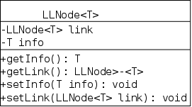
  public class LLStringNode {
    private String info;
    private LLStringNode link;
  }
Despite what was just said, the Java code on the right makes it
look as if a node does contain another node.
This confusion is caused by our friend reference semantics
.
Since LLStringNode is a class (and not a
primitive type), a variable of that type, such as link
shown on the right, is a reference, i.e., a pointer
(link corresponds to the Next box above;
info corresponds to Data).
The previous paragraph is important. It is a key to understanding linked data structures. Be sure you understand it.
  public LLStringNode(String info) {
    this.info = info;
    link = null;
  }
The LLStringNode constructor simply initializes the two fields. We set link=null to indicate that this node does not have a successor.
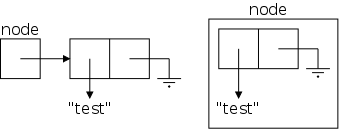
Forgive me for harping so often on the same point, but please be sure you understand why the constructor above, when invoked via the Java statement
node = new LLStringNode("test");
gives rises to the situation depicted on the near right and not the situation depicted on the far right.
Recall from 101 that all references are the same size. My house in the suburbs is much bigger than the apartment I had in Washington Square Village, but their addresses are (about) the same size.
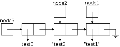
Now let's consider a slightly larger example, 3 nodes. We execute the Java statements
  node1 = LLStringNode("test1");
  node2 = LLStringNode("test2");
  node3 = LLStringNode("test3");
  node3.setLink(node2);
  node2.setLink(node1);
setLink() is the usual mutator that sets
the link field of a node.
Similarly we define setInfo(), getLink(),
and getInfo().
Homework: 41, 42.
Remark: In 2012-12 fall, this was assigned next lecture.
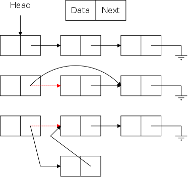
From the diagram on the right, which we have seen twice before, the Java code for simple linked list operations is quite easy.
The usual terminology is that you traverse
a
list, visiting
each node in order of its occurrence on the
list.
We need to be given a reference to the start of the list (Head in
the diagram) and need an algorithm to know when we have reached the
end of the list (the link component is null).
As the traversal proceeds each node is visited
.
The visit program is unaware of the list; it processes the Data
components only (called info in the code).
  public static void traverse(LLStringNode node) {
    while (node != null) {
      visit(node.getInfo());
      node = node.getLink();
    }
  }
Note that this works fine if the argument is null, signifying a list of length zero (i.e., an empty list).
Note also that you can traverse() a list starting at any node.
The bottom row of the diagram show the desired result of inserting an node after the first node. (The middle row shows deletion.) Two references are added and one (in red) is removed (actually replaced).
The key point is that to insert a node you need the red reference as well as a reference to the new node. In the picture the red reference is the Next field of a node. Another possibility is that it is an external reference to the first node (e.g. Head in the diagram). A third possibility is that the red reference is the null in the link field of the last node. Yet a fourth possibility is that the list is currently empty and the red reference is a null in Head.
However in all these cases the same two operations are needed (in this order).
We will see the Java code shortly.
Mosts list support deletion. However our stringlog example does not, perhaps because logs normally do not (or perhaps because it is awkward for an array implementation).
The middle row in the diagram illustrates deletion for (singly) linked lists. Again there are several possible cases (but the list cannot be empty) and again there is one procedure that works for all cases.
You are given the red reference, which points to the node to be deleted and you set it to the reference contained in the next field of the node to which it was originally pointing.
(For safety, you might want to set the original next field to null).
General lists support traversal as well as arbitrary insertions and deletions. For stacks, queues, and stringlogs only a subset of the operations are supported as shown in the following table. The question marks will be explaned in the next section.
| Insertion | Deletion | ||||||
|---|---|---|---|---|---|---|---|
| Structure | Traversal | Beginning | Middle | End | Beginning | Middle | End |
| Stringlog | XX | ?? | ?? | ||||
| Stack | XX | XX | |||||
| Queue | XX | XX | |||||
| General List | XX | XX | XX | XX | XX | XX | XX |
  package ch02.stringLogs;
  public class LinkedStringLog
         implements StringLogInterface { ... }
This new class LinkedStringLog implements the same ADT as did ArrayStringLog and hence its header line looks almost the same.
  private LLStringNode log;
  private String name;
We again have a name for each stringlog, but the first field looks
weird.
Why do we have a single node associated with each log?
It seems that all questions have the same answer:
reference semantics
.
An LLStringNode is not a node but a reference or pointer to a node. Referring to the pictures in the previous section, the log field corresponds to head in the picture and not to one of the horizontal boxes containing data and next components. If the declaration said LLStringNode log new LLStringNode(...), then log would still not be a horizontal box but would point to one. As written the declaration yields an uninitialized data field.
  public LinkedStringLog(String name) {
    this.name = name;
    log = null;
  }
An advantage of linked over array based implementations is that there is no need to specify (or have a default for) the maximum size. The linked structure grows as needed. This observation explains why there is no size parameter in the constructor.
As far as I can tell the log=null; statement could have be omitted if the initialization was specified in the declaration.
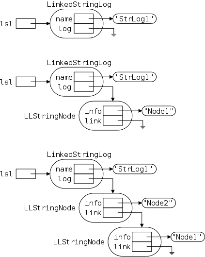
There are many names involved so a detailed picture may well prove helpful. Note that the rounded boxes (let's hope apple doesn't have a patent on this as well) are actual objects; whereas references are drawn as rectangular boxes. There are no primitive types in the picture.
Note also that all the references are the same size; but not all the objects. The names next to (not inside) an object give the type (i.e., class) of the object. To prevent clutter I did not write String next to the string objects, believing that the "" makes the type clear.
The first frame shows the result of executing
  LinkedStringLog lsl =
       new LinkedStringLog("StrLog1");
Let's go over this first frame and see that we understand every detail in it.
The other two frames show the result after executing
  lst.insert ("Node1");
  lst.insert ("Node2");
We will discuss them in a few minutes. First, we will introduce insert() with our familiar, much less detailed, picture and present the Java commands that do the work.
Note that the size of a LinkedStringLog and of an LLStringNode look the same in the diagram because they both contain two fields, each of which is a reference (and all references are the same size). This is just a coincidence. Some objects contain more references than do others; some objects contain values of primitive types; and we have not shown the methods associated with types.
An interesting question arises here that often occurs.
A liberal interpretation of the word log
permits a more
efficient implementation than would be possible for a stricter
interpretation.
Specifically does the term log imply that new entries are inserted
at the end of the log?
I think of logs as structures that are append only, but that was never stated in the ADT. For an array-based implementation, insertion at the end is definitely easier, but for linked, insertion at the beginning is easier.
However, the idea of a beginning and an end really doesn't apply to the log. Instead, the beginning and end are defined by the linked implementation. As far as the log is concerned, we can call either side of the picture the beginning.
The bottom row of the picture on the right shows the result of inserting a new element after the first existing element. For stringlogs we want to insert at the beginning of the linked list, so the red reference is the value of Head in the picture or log in the Java code.
  public void insert(String element) {
    LLStringNode node = new LLStringNOde(element);
    node.setLink(log);
    log = node;
  }
The code for insert() is very short, but does deserve
study.
The first point to make is that we are inserting at the beginning of
the linked list so we need a pointer to
the node before the first node
.
The stringlog itself serves as a surrogate for this pre-first
node.
Let's study the code using the detailed picture in the
An Example
section above.
  public void clear() {
    log = null;
  }
The clear() method simply sets the log back to initial state, with the node pointer null.
Start Lecture #6
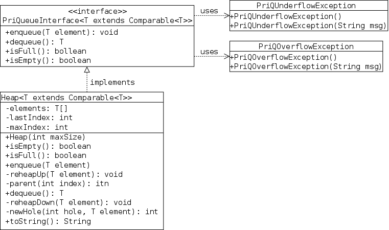
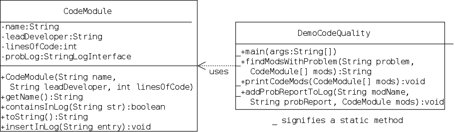
Remarks: I added a uses
arrow to the
diagram in section 2.B.
Redo insert using the new detailed diagram.
Homework: 41, 42.
Remark: This homework should have been assigned last lecture.
Lab: 2 assigned. It is due 2 October 2012 and includes an honors supplement.
  public boolean isFull() {
    return false;
  }
With a linked implementation, no list can be full.
Recall that the user may not know the implementation chosen or may wish to try both linked- and array- based stringlogs. Hence we supply isFull() even though it may never be used and will always return false.
  public String getName() {
    return name;
  }
getName() is identical for both the linked- and array-based implementations.
  public int size() {
    int count = 0;
    LLStringNode node = log;
    while (node != null) {
      count ++;
      node = node.getLink();
    }
    return count;
  }
The size() method is harder for this linked representation than for out array-based implementation since we do not keep an internal record of the size and must traverse the log as shown on the right
An alternate implementation would be to maintain a count field and have insert() increment count by 1 each time.
One might think that the alternate implementation is better for the following reason. Currently insert() is O(1) and size() is O(N). For the alternative implementation both are O(1). However, it is not that simple, the number of items that size() must count is the number of inserts() that have been done, so there could be N insert()'s for one size().
A proper analysis is more subtle.
  public String toString() {
    String ans = "Log: " + name + "\n\n";
    int count = 0;
    for (LLStringNode node=log; node!=null; node=node.getLink())
      ans = ans + (++count) + ". " + node.getInfo() + "\n";
    return ans;
  }
The essence of toString() is the same as for the array-based implementation. However, the loop control is different. The controlling variable is a reference, it is advanced by getLink() and termination is a test for null.
  public boolean contains(String str) {
    for (LLStringNode node=log; node!=null; node=node.getLink())
      if (str.equalsIgnoreCase(node.getInfo()))
        return true;
    return false;
  }
Again the essence is the same as for the array-based implementation, but the loop control is different. Note that contains() and toString() have the same loop control. Indeed, advancing by following the link reference until it is null is quite common for any kind of linked list.
The while version of this loop control was used in size().
Homework: 44, 47, 48.
Read
Read
A group is developing a software system that is comprised of several modules, each with a lead developer. They collect the error messages that are generated during each of their daily builds. Then they wish to know, for specified error messages, which modules encountered these errors.
I wrote a CodeModule class that contains the data and methods for one code module, including a stringlog of its problem reports. This class contains
This is not a great example since stringlogs are not a perfect fit. I would think that you would want to give a key word such as documentation and find matches for documentation missing and inadequate documentation . However, stringlogs only check for (case-insensitive) complete matches.
The program reads three text files.
Let's look at the UML and sketch out how the code should be constructed. Hand out the UML for stringlogs. The demo class could be written many ways, but we should pretty much all agree on CodeModule.java.
The Java programs, as well as the data files, can be found here.
Note that program is a package named codeQuality. Hence it must live in a directory also named codeQuality. To compile and run the program, I would be in the parent directory and execute.
  export CLASSPATH=/a/dale-dataStructures/bookFiles:.
  javac codeQuality/DemoCodeQuality.java
  java codeQuality/DemoCodeQuality
You would do the same but the replace /a/dale-dataStructures/BookFiles by wherever you downloaded the book's packages.
It is important to distinguish the user's and implementers view of data structures. The user just needs to understand how to use the structure; whereas, the implementer must write the actual code. Java has facilities (classes/interfaces) that make this explicit.
Start Lecture #7
We will now learn our first general-purpose data structure, taking a side trip to review some more Java.
Definition: A stack is a data structure from which one can remove or retrieve only the element most recently inserted.
This requirement that removals are restricted to the most recent insertion implies that stacks have the well-known LIFO (last-in, first-out) property.
In accordance with the definition the only methods defined for stacks are push(), which inserts an element, pop(), which removes the most recently pushed element still on the stack, and top(), which retrieves (but does not remove) the most recently pushed element still on the stack.
An alternate approach is to have pop() retrieve as well as remove the element.
Stacks are a commonly used structure, especially when working with data that can be nested. For example consider evaluating the following postfix expression (or its infix equivalent immediately below).
  22 3 + 8 * 2 3 4 * - -
  ((22 + 3) * 8) - (2 - 3 * 4))
A general solution for infix expressions would be challenging for us, but for postfix it is easy!
Homework: 1, 2
In Java a collection represents a group of objects, which are called the collections's elements. A collection is a very general concept that can be refined in several ways. We shall see several such refinements.
For example, some collections permit duplicates; whereas others do not. Some collections, for example, stacks and queues, restrict where insertions and deletions can occur. In contrast other collections are general lists, which support efficient insertion/deletion at arbitrary points.
Last semester I presented a sketch of these concepts as an optional topic. You might wish to read it here.
Our ArrayStringLog class supports a collection of Strings. It would be easy, but tedious, to produce a new class called ArrayIntegerLog that supports a collection of Integers. It would then again be easy, but now annoying, to produce a third class ArrayCircleLog, and then ArrayRectangleLog, and then ... .
If we needed logs of Strings, and logs of Circles, and logs of Integers, and logs of Rectangles, we could cut the ArrayStringlog class, paste it four times and do some global replacements to produce the four needed classes. But there must be a better way!
In addition this procedure would not work for a single heterogeneous log that is to contain Strings, Circles, Integers, and Rectangles.
  public class T {
    ...
  }
  public class S extends T {
    ...
  }
  public class Main {
    public static void main(String[] args) {
      T t;
      S s;
      ...
      t = s;
    }
  }
Recall from 101 that a variable of type T can be assigned a value from any class S that is a subtype of T.
For example, consider three files T.java, S.java, and Main.java as shown on the right. We know that the final assignment statement t=s; is legal; whereas, the reverse assignment s=t; may be invalid;
When applied to our ArrayStringLog example, we see that, if we developed an ArrayObjectLog class (each instance being a log of Java objects) and constructed objLog as an ArrayObjectLog, then objLog could contain three Strings, or it could contain two Circles, or it could contain four Doubles, or it could contain all 9 of these objects at the same time.
For this heterogeneous example where a single log is to contain items of many different types, ArrayObjectLog is perfect.
As we just showed, an ArrayObjectLog can be used for either homogeneous logs (of any type) or for heterogeneous logs. I asserted it is perfect for the latter, but (suspiciously?) did not comment on its desirability for the former.
To use ArrayObjLog as the illustrative example, I must extend it a little. Recall that all these log classes have an insert() method that adds an item to the log.. Pretend that we have augmented the classes to include a retrieve() method that returns some item in the log (ignore the possibility that the log might be empty). So the ArrayStringLog method retrieve() returns a String, the ArrayIntegerLog method retrieve() returns an Integer, the ArrayObjectLog method retrieve() returns an Object, etc.
Recall the setting. We wish to obviate the need for all these log classes except for ObjectLog, which should be capable of substituting for any of them. The code on the right uses an ObjectLog to substitute for an IntegerLog.
  ArrayObjectLog integerLog =
                 new ArrayObjectLog("Perfect?");
  Integer i1=5, i2;
  ...
  integerLog.insert(i1);         // always works
  i2 = integerLog.retrieve();   // compile error
  i2 = (Integer)integerLog.retrieve();  // risky
  Object o = integerLog.retrieve();
  if (o instanceof Integer)
    i2 = (Integer)o;                    // safe
  else
    // What goes here?
    // Answer:  A runtime error msg
    // or a Java exception (see below).
Java does not know that this log will contain only Integers so a naked retrieve() will not compile.
The downcast will work providing we in fact insert() only Integers in the log. If we erroneously insert something else, retrieve()d will generate a runtime error that the user may well have trouble understanding, especially if they do not have the source code.
Using instanceof does permit us to generate a (hopefully) informative error message, and is probably the best we can do. However, when we previously used a real ArrayIntegerLog no such runtime error could occur, instead any erroneous insert() of a non-Integer would fail to compile. This compile-time error is a big improvement over the run-time error since the former would occur during program development; whereas, the latter occurs during program use.
Summary: A log of Objects can be used
for any log; it is perfect for heterogeneous logs, but
can degrade
compile-time error into run-time errors for
homogeneous logs.
We will next see a perfect
solution (using Java
generics) for homogeneous logs.
Homework: 4.
Recall that ArrayStringLog is great for logs of Strings, ArrayIntegerLog is great for logs of Integers, etc. The problem is that you have to write each class separately even though they differ only in the type of the logs (Strings, vs Integers, vs etc). This is exactly the problem generics are designed to solve.
The idea is to parameterize the type as I now describe.
  y1 = tan(5.1) + 5.13 + cos(5.12)
  y2 = tan(5.3) + 5.33 + cos(5.32)
  y3 = tan(8.1) + 8.13 + cos(8.12)
  y4 = tan(9.2) + 9.23 + cos(9.22)

  f(x) = tan(x) + x3 + cos(x2)
  y1 = f(5.1)
  y2 = f(5.3)
  y3 = f(8.1)
  y4 = f(9.2)
It would be boring and repetitive to write code like that on the top right (using mathematical not Java notation).
Instead you would define a function that parameterizes the numeric value and then invoke the function for each value desired. This is illustrated inn the next frame.
Compare the first y1 with f(x) and note that we replaced each 5.1 (the numeric value) by x (the function parameter). By then invoking f(x) for different values of the argument x we obtain all the ys.
In our example of ArrayStringLog and friends we want to
write one parameterized
class (in Java it would be called
a generic class and named ArrayLog<T>,
with T the type parameter) and then instantiate
the parameter
to String, Integer, Circle, etc. to
obtain the equivalent of ArrayStringLog,
ArrayIntegerLog, ArrayCircleLog, etc.
  public class ArrayLog<T> {
    private T[] log;
    private int lastIndex = -1;
    private String name;
    ...
  }
In many (but not all) places where ArrayStringLog had String, ArrayLog<T>, would have T. For example on the right we see that the log itself is now an array of Ts, but the name of the log is still a String.
We then get the effect of ArrayStringLog by writing ArrayLog<String>. Similarly we get the effect of ArrayIntegerLog by writing ArrayLog<Integer>, etc.
  public interface LogInterface<T> {
    void insert(T element);
    boolean isFull();
    int size();
    boolean contains(T element);
    void clear();
    String getName();
    String toString();
  }
In addition to generic classes such as ArrayLog<T>, we can also have generic interfaces such as LogInterface<T>, which is shown in its entirety on the right. Again note that comparing LogInterface<T> with StringLogInterface from the book, we see that some (but not all) Strings have been changed to Ts, and <T> has been added to the header line.
We will see several complete examples of generic classes as the course progresses.
The current situation is pretty good.
What's left?
Assume we want to keep the individual entries of the log is some order, perhaps alphabetical order for Strings, numerical order for Integers, increasing radii for circles, etc.
For this to occur, the individual items in the log must
be comparable
, i.e, you must be able to decide which of two
items comes first
.
This requirement is a restriction on the possible types that can be
assigned to T.
As it happens Java has precisely the notion that elements of a type can be compared to each other. The requirement is that the type extends the standard library interface called Comparable. Thus to have sorted logs, the element type T must implement the Comparable interface. In Java an array-based version would be written (rather cryptically) as
public class ArrayLog<T extends Comparable<T>> { ... }
We are not yet ready to completely understand that cryptic header.
We covered Java exceptions in 101 so this will be a review.
As a motivating example consider inserting a new log into a full ArrayStringLog. Our specification declared this to be illegal, but nonetheless, what should we do? The key point is that the user and not the implementer of ArrayStringLog should decide on the action. Java exceptions make this possible as we shall see.
An exceptional situation is an unusual, sometimes unpredictable event. It need not be fatal, but often is, especially if not planned for. Possibilities include.
impossibleoperation, such as popping an empty stack (which well cause an illegal array reference).
We will see that Java (and other modern programming languages) has support for exceptional conditions (a.k.a. exceptions). This support consists of three parts.
As we shall see an exception can be thrown from one piece of code and caught somewhere else, perhaps in a place far, far away.
This section is from my 101 class notes.
double s12 = p1.distTo(p2);
if (s12!=p2.distTo(p3) || s12!=p3.distTo(p4) ||
    s12!=p4.distTo(p1)) {
  System.out.println("Error: Rhombus with unequal sides");
  System.exit(0);       // an exception would be better
}
sidelength = s12;


double s12 = p1.distTo(p2);
try {
  if (s12!=p2.distTo(p3) || s12!=p3.distTo(p4) ||
      s12!=p4.distTo(p1))
    throw new Exception("Rhombus with unequal side");
  sidelength = s12;
}
catch (Exception ex) {
  System.out.println("Error: Rhombus with unequal sides");
  System.exit(0);
}
The top frame on the right shows (a slight variant of) the body of the Rhombus constructor. This constructor produces a rhombus given its four vertices. It terminates the run if the parameters are invalid (the side lengths are not all equal).
The frame below it shows one way to accomplish the same task using an exception. There are four Java terms introduced try, throw, catch, and Exception.
try and catch each introduce a block of code, which are related as follows.
matching(explained later) catch block is executed.
In the example code, if all the side lengths are equal, sidelength is set. If they are not all equal an exception in the class Exception is thrown, sidelength is not set, an error message is printed and the program exits.
This behavior nicely mimics that of the original, but is much more complicated. Why would anyone use it?
The answer to the above question is that using exceptions in the manner of the previous section to more-or-less exactly mirror the actions without an exception is not a good idea.
Remember the problem with the original solution. The author of the geometry package does not know what the author of the client wants to do when an error occurs (forget that I was the author of both). Without any such knowledge the package author terminated the run as there was no better way to let the client know that a problem occurred.
The better idea is for the package to detect the error, but let the client decide what to do.
The first step is to augment the Rhombus class with a constructor having three parameters: a point, a side-length, and an angle. The constructor produces the rhombus shown on the right (if Θ=Π/2, the rhombus is a square).
 public Rhombus (Point p, double sideLength, double theta) {
   super (p,
          new Point(p.x+sideLength*Math.cos(theta),
                    p.y+sideLength*Math.sin(theta)),
          new Point(p.x+sideLength*(Math.cos(theta)+1.),
                    p.y+sideLength*Math.sin(theta)),
          new Point(p.x+sideLength, p.y));
   this.sideLength = sideLength;
 }


 double s12 = p1.distTo(p2);
 if (s12!=p2.distTo(p3) || s12!=p3.distTo(p4) || s12!=p4.distTo(p1))
   throw new Exception ("Rhombus with unequal sides.");
 sideLength = s12;


 try {
   rhom1 = new Rhombus(origin,origin,p2,p3);
 }
 catch (Exception ex) {
   System.out.printf("rhom1 error: %s  Use unit square.\n",
                     ex.getMessage());
   rhom1 = new Rhombus (origin, 1.0, Math.PI/2.0);
 }
The constructor itself is in the 2nd frame.
This enhancement has nothing to do with exceptions and could have
(perhaps should have) been there all along.
You will see below how this standard rhombus
is used when the
client mistakenly attempts to construct an invalid rhombus.
The next step, shown in the 3rd frame, is to have the regular rhombus constructor throw an exception, but not catch it.
The client code is in the last frame. We see here the try and catch. In this frame the client uses the original 4-point rhombus constructor, but the points chosen do not form a rhombus. The constructor detects the error and raises (throws in Java-speak) an exception. Since the constructor does not catch this exception, Java automatically re-raises it in the caller, namely the client code, where it is finally caught. This particular client chooses to fall back to a unit square.
It is this automatic call-back provided by exceptions that enables the client to specify the action required.
Read the book's (Date) example, which includes information on creating exceptions and announcing them in header lines.
A Java exception is an object that is a member of either Exception, Error, or a subclass of one of these two classes.
throw new Exception ("Rhombus with unequal sides.");
On the right is the usage from my rhombus example above. As always the Java keyword new creates an object in the class specified. In the example, we do not name this object. We simply throw it.
  public class GeometryException extends Exception {
    public GeometryException() { super(); }
    public GeometryException(String msg) { super(msg); }
  }
For simplicity, our example created an Exception. It is often convenient to have different classes of exceptions, in which case you would write code as shown on the right. This code creates a new subclass of Exception and defines two constructors to be the same as for the Exception class itself. (Recall that super() in a constructor invokes a constructor in the superclass.)
  throw new GeometryException
        ("Rhombus with unequal sides.");
We would then modify the throw to create and raise an exception in this subclass.
We have seen that if an exception is raised in a method and not caught there, the exception is re-raised in the caller of the method. If it is also not caught in this second method, it is re-raised in that method's caller. This keeps going and if the exception is not caught in the main method, the program is terminated. Note that if f() calls g() calls h() calls k() and an exception is raised in k(), the handler (the code inside catch{}) is searched for first in k(), then h(), then g(), and then f(), the reverse order of the calling sequence.
In this limited sense, exceptions act similar to returns.
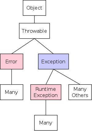
There is one more point that we need to review about exceptions and that is their (often required) appearance in method header lines. To understand when header line appearance is required, we examine the color coded class tree for Java exceptions shown on the right.
As always, Object is the root of the Java class tree and naturally has many children in addition to Throwable. As the name suggests, the Throwable class includes objects that can be thrown, i.e., Java exceptions.
For us, there are three important classes of pre-defined exceptions highlighted in the diagram: namely Error, Exception, and RuntimeException.
The red exceptions (and their white descendants)
are called unchecked exceptions
; the blue exceptions (and
their remaining white descendants) are called
checked exceptions
.
The header line rule is now simple to state (but not as simple to
apply):
Any method that might raise a checked exception
must announce this fact in its header line using
the throws keyword.
For example, the rhombus constructor would be written as follows.
  public Rhombus (Point p1, Point p2, Point p3, Point p4) throws Exception {
    super(p1, p2, p3, p4);  // ignore this; not relevant to exceptions
    double s12 = p1.distTo(p2);
    if (s12!=p2.distTo(p3) || s12!=p3.distTo(p4) || s12!=p4.distTo(p1))
      throw new Exception ("Rhombus with unequal sides.");
    sideLength = s12;
  }
The slightly tricky part comes when f() calls g(), g() calls h(), and h() raises a checked exception that it does not catch. Clearly, the header line of h() must have a throws clause. But, if g() does not catch the exception, then it is reraised in f() and hence g() must have a throws clause in its header line as well.
The point is that a method (g() above) can raise an exception even though it does not itself have a throw statement.
This makes sense since from the point of view of the caller of g() (method f() in this case), method g() does raise an exception so g() must announce that in its header.
When a method detects an error, three possible actions can occur.
Homework: 8.
We know that a stack is a list with LIFO (last-in, first-out) semantics and that it has three basic operations.
We choose to specify and implement a generic (homogeneous) stack. That is all elements of a given stack are of the same type, but different stacks can have elements of different type.
We use T for the element type, so our generic stack interface will be StackInterface<T>.
This is clearly an error so something must be done. We could simply add to the specification that top() and pop() cannot be called when the stack is empty, but that would be a burden for the client (even though we will supply an isEmpty() method).
We could try to handle the error in the pop() and top() methods themselves, but it is hard to see what would be appropriate for all clients. This leads to the chosen solution, an exception.
Our stack class will raise an exception when either top() or pop() is called when the stack is empty.
Rather that just using the Exception class, we will define our own exception. This immediately raises two questions: what should we name the exception and should it be checked or unchecked.
  package ch03.stacks;
  public class StackUnderFlowException
         extends RuntimeException {
    public StackUnderFlowException() {
      super();
    }
    public StackUnderFlowException(String msg) {
      super(msg);
    }
  }

  public class SUE extends RTE {
    public SUE() { super(); }
    public SUE(String msg) { super(msg); }
  }
The book names it StackUnderflowException as shown in the first frame on the right. A corresponding exception in the Java library is called EmptyStackException. A good feature of long names like these is that they are descriptive. A downside is that the code looks longer. Don't let the extra length due to the long names lead you to believe the situation is more complicated than it really is.
The second frame shows the same code assuming the exception was named SUE, and assuming that Java used RTE rather than RuntimeException, and omitting the package statement, which has nothing to do with the exception itself.
I am definitely not advocating short cryptic names; just pointing out how simple the StackUnderFlowException really is.
A more serious question is whether the exception should be checked or unchecked, i.e., whether it should extend Exception or RuntimeException.
  import ch03.stacks.*;
  public class DemoStacks {
    public static void main(String[] args) {
      ArrayStack<Integer> stack =
        new ArrayStack<Integer>();
      Integer x = stack.top();
    }
  }
The code on the right shows the disadvantage of an unchecked exception. This simple main program creates an empty stack (we will learn ArrayStack soon) and then tries to access the top member, a clear error.
As we shall see, the code in top() checks for an empty stack and raises the StackUnderflowException when it finds one. Since top() does not catch the exception, it is reraised in the JVM (the environment that calls main() and a runtime error message occurs. Were the exception checked, the program would not compile since the constructor can throw a checked exception, which the caller neither catches nor declares in its header. In general compile time errors are better than runtime errors.
  import ch03.stacks.*;
  public class DemoStacks {
    public static void main(String[] args) {
      ArrayStack<Integer> stack =
        new ArrayStack<Integer>();
      stack.push(new Integer(3));
      Integer x = stack.top();
    }
  }
The very similar program on the right, however, shows the advantage of an unchecked exception. This time, the stack is not empty when top() is called and hence no exception is generated. This program compiles and runs with no errors. However, if the exception were checked, the program again would not compile, adding try{} and catch{} blocks would clutter the code, and a header throws clause, would be a false alarm.
The try{}...catch{} block pair can always be used as can the header throws clause. The choice between checked and unchecked errors is whether clients should be required or simply permitted to use these mechanisms.
A somewhat, but not completely, analogous situation occurs when trying to push an item onto a full stack. The reason the situation is not truly analogous is that conceptually, although a stack can be empty, it cannot be full.
Some stack implementations, especially those based on arrays, do produce stacks with an upper bound on the number of elements they can contain. Such stacks can indeed be full and these implementations supply both an isFull() method and a StackOverflowException exception.
  public class SOE extends RTE {
    public SOE() { super(); }
    public SOE(String msg) { super(msg); }
  }
On the right is the corresponding StackOverflowException
class, written in the same
abbreviated
style used above.
Note how stylized these exception definitions are.
Written in the abbreviated style, just three U's were changed to
O's.
Homework: 17.
Start Lecture #8
Remark: Give a better answer to class T extends S {} T t; S s; t=s; s=t;
Question: Do we tell clients that there is an isFull() method and mention the StackOverflowException that push() might raise? Specifically, should we put them in the interface?
If we do, then implementations that can never have a full stack, must implement a trivial version of isFull(). If we don't, then how does the client of an implementation that can have full stacks, find out about them?
One can think of several solutions: comments in the interface describing the features in only some implementations, a separate document outside Java, etc
We shall follow the book and use a hierarchy of three Java interfaces.
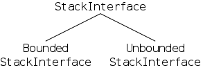
  package ch03.stacks;
  public interface StackInterface<T> {
    void pop() throws StackUnderflowException;
    T    top() throws StackUnderflowException;
    boolean isEmpty();
  }
On the right we see the basic interface for all stacks. It is parameterized by T the type of the elements in the stack.
The interface specifies one mutator, two accessors, and one possibly thrown exception. Two points deserve comment.
  package ch03.stacks;
  public interface BoundedStackInterface<T>
      extends StackInterface<T> {
    void push(T element)
      throws StackOverflowException;
    boolean isFull();
  }
The first item to note concerning the code on the right is the extends clause. As with classes one interface can extend another. In the present case BoundedStackInterface inherits the three methods in StackInterface.
Since this extended interface is to describe stacks with an upper bound on the number of elements, we see that push() can raise an overflow exception. A predicate is also supplied so that clients can detect full stacks before causing an exception.
  package ch03.stacks;
  public interface UnboundedStackInterface<T>
      extends StackInterface<T> {
    void push(T element);
  }
Perhaps the most interesting point in this interface is the observation that, although it might be a little harder to implement a stack without a bound, it is easier to describe. The concept of a full stack and the attendant exception, simply don't occur.
This simpler description suggests that the using an unbounded stack will be slightly easier than using a bounded one.
Imagine your friend John hands you three plates, a red, then a white, and then a blue. As you are handed plates, you stack them up. When John leaves, Mary arrives and you take the plates off the pile one at a time and hand them to Mary. Note that Mary gets the plates in the order blue, white, red the reverse from the order you received them.
It should be no surprise that this algorithm performs the same for Integers as it does for plates (it is what we would call a generic method. The algorithm is trivial push...push pop...pop.
import ch03.stacks.*;
import java.util.Scanner;
public class ReverseIntegers {
  public static void main(String[] args) {
    Scanner getInput = new Scanner(System.in);
    int n = getInput.nextInt(), revInt;
    BoundedStackInterface<Integer> stack =
      new ArrayStack<Integer>(n);
    for (int i=0; i<n; i++)
      stack.push(new Integer(getInput.nextInt()));
    for (int i=0; i<n; i++) {
      revInt = stack.top();  stack.pop();
      System.out.println(revInt);
    }
  }
}
A few comments on the Integer version shown on the right.
Homework: 18.
To help summarize the code in this chapter, here is the UML for the entire stack package
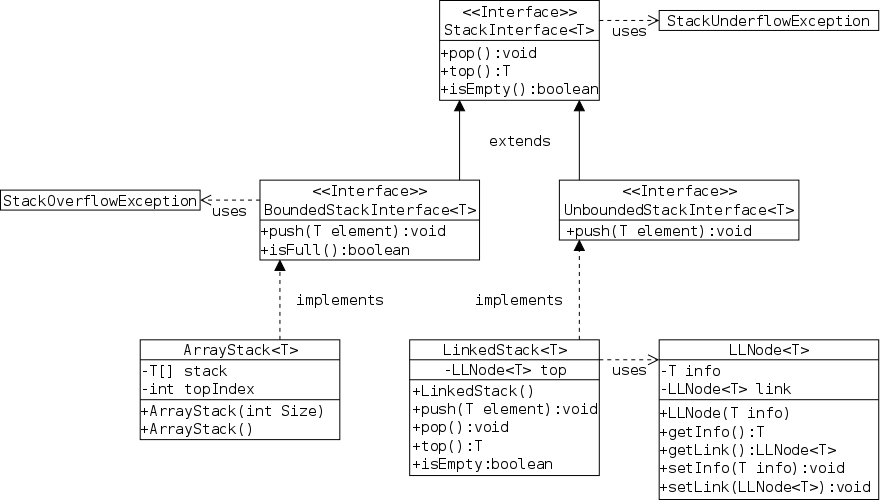
It is important not to let the fancy Java in this chapter (including more to come) hide the fact that implementing a stack with an array arr and an index idx is trivial: push(x) is basically arr[idx++]=x, top() is basically return arr[idx], and pop() is basically idx--.
The idea is that the elements currently in the stack are stored in the lowest indices of the array. We need to keep an index saying how much of the array we have used. The book has the index refer to the highest array slot containing a value; a common alternative is to have the index refer to the lowest empty slot; a frequent error is to do a little of each.
  package ch03.stacks;
  public class ArrayStack<T>
      implements BoundedStackInterface<T> {
    private final int DEFSIZE = 100;
    private T[] stack;
    private int topIndex = -1;
    public ArrayStack(int size) {
      stack = (T[]) new Object[size];
    }
    public ArrayStack() { this(DEFSIZE); }
The beginning of the class is shown on the right. We see from the header that it is generic and will implement all the methods in BoundedStackInterface (including those in StackInterface).
I changed the visibility of the fields from protected to private since I try to limit visibilities to private fields and public methods. I also used this to have the no-arg constructor invoke the 1-arg constructor.
I could spend half a lecture on the innocent
looking assignment to stack, which should
be
simply new T[size].
Unfortunately, that simple code would not compile, due to a weakness
in the Java implementation of generics, which does not permit the
creation of generic arrays (although it does permit their
declaration as we see on the right).
There is even a mini controversy as to why the weakness exists.
Accepting that new T[size] is illegal, the given code creates an array of Objects and downcasts it to an array of T's. For complicated reasons having to do with Java's implementation of generics, the downcast creates a warning claiming that it can't be sure the created array will be used correctly in all situations. We shall sadly have to accept the warning.
  public boolean isEmpty() { return topIndex == -1; }
  public boolean isFull()  { return topIndex == stack.length-1; }
For some reason the authors write these using if-then-else, converting trivial 1-liners into trivial 4-liners.
  public void push(T element) {
  if (isFull())
    throw new StackOverflowException("helpful msg");
  else
    stack[++topIndex] = element;
  }

  public void pop() {
  if (isEmpty())
    throw new StackUnderflowException("helpful msg");
  else
    stack[topIndex--] = null;
  }

  public T top() {
  if (isEmpty())
    throw new StackUnderflowException("helpful msg");
  else
    return stack[topIndex];
  }
These three methods, two mutators and one accessor, are the heart of the array-based stack implementation. As can be seen from the code on the right all are trivial.
pop() is not required to set the top value null. It is a safety measure to prevent inadvertently referring stale data.
My code assumes knowledge of the Java (really C) increment/decrement operators ++ and -- used both as prefix and postfix operators. The authors avoid using these operators within expressions, producing slightly longer methods. This result is similar to their using an if-then-else rather than returning the value of the boolean expression directly. I believe that Java programmers should make use of these elementary features of the language and that they quickly become idiomatic.
Homework: 28, 30
Read.
The interesting part of this section is the ArrayList class in the Java library. An ArrayList object has the semantics of an array that grows and shrinks automatically; it is never full. When an ArrayList used in place of an array, the resulting stack is unbounded. This library class is quite cool.
The essential point of well-formed expressions is that (all forms of) parentheses are balanced. So ({({[]})}) is well-formed, but ({({[]}})) is not. Note that we are concerned only with the parentheses so ({({[]})}) is the same as ({xds(45{g[]rr})l}l).
Why are stacks relevant?
When we see an open parenthesis, we stack it and continue. If we see another open, we stack it too. When we encounter a close it must match the most recent open and that is exactly the top of stack.
The authors present a more extensive solution than I will give. Their Balanced class permits one to create an object that checks balanced parentheses for arbitrary parentheses.
  new Balanced("([{", ")]}")
  new Balanced("]x*,", "[y3.")
This approach offers considerable generality. The top invocation on the right constructs a Balanced object that checks for the three standard pairs of parentheses used above. The second invocation produces a weird object that checks for four crazy pairs of parentheses "][", "xy", "*3", and ",.".
  For each input char
    if open,    push
    if close,   pop and compare
    if neither, ignore
  When finished, stack must be empty
Since the purpose is to illustrate the use of stack and I would like us to develop the code in class, let me simplify the problem a little and just consider ([{ and )]}. Also we require a whitespace between elements so that we can use the scanner's hasNext() and getNext() methods. With this simplification a rough description of the algorithm is on the right. A complete Java solution is here.
Start Lecture #9
Modern versions of Java, will automatically convert between an int and an Integer. This comes up in the book's solution for balanced parentheses since they push indices (int's not String's. Although we didn't need it, this autoboxing and autounboxing is quite useful and requires some comment.
The point is that int is a primitive type (not a class) so we cannot say ArrayStack<int> to get a stack of int's. The closest we can get is ArrayStack<Integer>.
  stack.push(new Integer(i1));

  stack.push(i1);
Assume stack is a stack of Integer's, and we want to push the value of an int variable i1. In older versions of Java, we would explicitly convert the int to an Integer by using a constructor as in the top line on the right. However Java 1.5 (current is 1.7) introduced the automatic conversion so we can use the bottom line on the right.
Homework: 36, 37(a-d).
As with StringLogs, both array- and link-based stack implementations are possible. Unlike arrays (but like ArrayLists), the linked structure cannot be full or overflow so it will be an implementation of UnboundedStackInterface.
  package support;
  public class LLNode<T> {
    private LLNode<T> link = null;
    private T info;
    public LLNode (T info) { this.info = info; }
    public T getInfo() { return info; }
    public LLNode<T> getLink() { return link; }
    public void setInfo(T info) { this.info = info; }
    public void setLink(LLNode<T> link) { this.link = link; }
  }
Essentially all linked solutions have a self-referential
node class with each node containing references to another node (the
link) and to some data that is application specific.
We did a specific case when implementing linked stringlogs.
A generic solution is on the right. The constructor is given a reference to the data for the node. Each of the two fields can be accessed and mutated, yielding the four shown methods.
Probably the only part needing some study is the use of genericity.
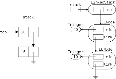
To motivate the implementation, on the far right is a detailed view of what should be the result of executing
  UnboundedStackInterface<Integer> stack =
            new LinkedStack<Integer> ();
  stack.push(new Integer(10));
  stack.push(20);    // autoboxed
Remember that the boxes with rounded corners are objects and their class names is written outside the box. The rectangles contain references.
Normally, much less detail is shown than we see on the far right. Instead, one would draw a diagram like the one on the near right.
Do not let schematic pictures like this one trick you into
believing that the info field contains an int such as 20.
It cannot.
The field contains a T and T is
never int.
Why?
Answer: T must be a class; not a
primitive type.
  package ch03.stacks;
  import support.LLNode;
  public class LinkedStack<T> implements
      UnboundedStackInterface<T> {
    private LLNode<T> top = null;
    ...
  }
Since LLNode will be used in several packages, it is
placed in separate package and imported here.
The alternative is to replicate LLNode in every package
using it; a poor idea.
Why?
Answer: Replicated items require care to ensure
changes are made to all copies.
The only data field is top, which points to the current top of stack.
An alternative to the field initialization shown would be to place write a constructor and place the initialization there. The book uses this alternative; the code shown does not need an explicit constructor, the no-arg constructor suffices.
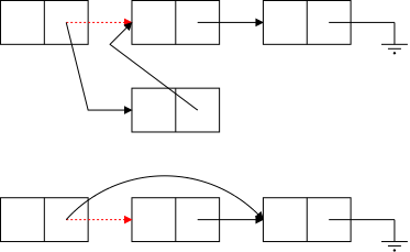
On the right is a schematic view of the actions needed to insert a node onto an arbitrary linked list and to delete a node from such a linked list. For a stack, these operations correspond to push and pop respectively.
There is a potential point of confusion, due in part to terminology, that I wish to explain.
Recall that, for a stack, the list head (commonly called top) is the site for all insertions and for all deletions. This means that new nodes are inserted before the current first node and hence the new node becomes the first node.
As a result, if node A is inserted first and node B is inserted subsequently, then, although node A's insertion was temporally prior to node B's, node A appears after node B on the stack (i.e., access to node A comes after access to node B.
This ordering on the list gives the LIFO (last-in, first-out) behavior required for a stack.
The push() operation corresponds to the first line in the diagram above. The only difference is that we are inserting before the current first node so the red dashed pointer is the contents of the top field rather than the link field of a node.
  public void push (T info) {
    LLNode<T> node = new LLNode<T>(info);
    node.setLink(top);
    top = node;
  }
From the diagram we see that the three steps are to create a new node, set the new link to the red link, and update the red link to reference the new node. Those three steps correspond one for one with the three lines of the method. A common error is to reverse the last two lines.
Show in class why reversing the last two lines fails.
Show in class that push() works correctly if the stack is empty when push() is called.
  public void pop() throws StackUnderflowException {
    if (isEmpty())
      throw new StackUnderflowException("helpful msg");
    else
      top = top.getLink();
  }
pop() corresponds to the second line of our diagram, again with the red pointer emanating from top, not from a node. So we just need to set the red arrow to the black one.
If the stack is empty, then the red arrow is null and there is no black arrow. In that case we have an underflow.
  public T top() {
    if isEmpty()
      throw new StackUnderflowException("helpful msg");
    else
      return top.getInfo();
  }


  public boolean isEmpty() { return top==null; }
top() simply returns the top element of the stack. If the stack is empty, an underflow is raised.
We must remember however that from the user's viewpoint, the stack consists of just the info components. The business with links and nodes is there only for our (the implementer's) benefit. Hence we apply getInfo().
Finally, a linked stack is empty if it's top field is null. Thus isEmpty() is a one-line method.
Both ArrayStack and LinkedStack are fairly simple and quite fast. All of the operations in both implementations are O(1), they execute only a fixed number of instructions independent of the size of the stack.
Note that the previous statement means that each push() takes only a constant number of instructions. Naturally pushing 1,000 elements takes longer (about 1000 times longer) than pushing one item.
The array-based constructor that is given the size of the array is not O(1) because creating an array of N Objects requires setting each of the N references to null. The linked-based constructor is O(1), which is better. Nonetheless, in a practical sense, both implementations are fast.
The two notable differences are
Homework: 40, 41, 45.
As mentioned at the beginning of this chapter, our normal arithmetic notation is called infix because the operator is in between the operands. Two alternatives notations are prefix (operator precedes the operands) and postfix (operator follows the operands).
As we know, with infix notation, some form of precedence rules are needed and often parentheses are needed as well. Postfix does not need either.
The evaluation rule is to push all operands until an operator is encountered in which case the operator is applied to the top two stacked elements (which are popped) and then the result is pushed (pop, pop, eval, pop).
Do several examples in class
The real goal is simply a method that accepts a postfix expression (a Java String) and returns the value of the expression. However, we cannot compile a naked method since, unlike some other languages, Java requires that each source file must be a class. Thus our goal will be a class containing a static method that evaluates postfix expressions. The class can be thought of as a simple wrapper around the method.
Read.
  import ch03.stacks.*;
  import java.util.Scanner;
  public class PostfixEval {
    public static double postfixEval(String expr) {
      ...
    }
  }
As mentioned, we want to develop the method postfixEval(), but must package it as a class, which we have called PostfixEval. The skeleton is on the right, let's write the ... part in class.
For simplicity, we assume the argument to postfixEval() is a valid postfix expression.
A solution is here and a main program is here. The latter assumes each postscript expression is on a separate line.
  export CLASSPATH="/a/dale-dataStructures/bookFiles/:."
  javac DemoPostfixEval.java
  java DemoPostfixEval
As a reminder this two-Java-files program can be compiled and run two ways. As written the program does not specify a package (technically it specifies the default package) so to compile and run it, go to its directory and execute the statements on the right.
  export CLASSPATH="/a/dale-dataStructures/bookFiles/:."
  javac postfixEval/DemoPostfixEval.java
  java postfixEval/DemoPostfixEval
Alternatively (and good practice) is to use a named package. For example, add package postfixEval; at the top of each file, make sure the directory is also named postfixEval, go the parent of this directory and type the commands on the right.
Read.
Read. The book does not assume the postfix expression is valid so testing is more extensive than we would require.
Homework: 48, 49.
Several points were made in this chapter.
A recursive definition defines something in terms of (a hopefully simpler version of) itself.
It is easier to write this in elementary mathematics than Java. Consider these examples in order and only consider integer arguments.
For each of the following, can you evaluate f(3)? How about f(-8)? How about f(n) for all integers n?
  1. f(n) = 1 + f(n-1)

  2. f(n) = 1 + f(n-1)  for n > 0
          = 0           for n ≤ 0    (base case)

  3. f(n) = 1 + f(n-1)  for n > 0
     f(0) = 0
     f(n) = 1 + f(n+1)  for n < 0

  4. f(n) = 1 + g(n)
     g(n) = 1 + f(n-1)  for n > 0
     g(0) = 0
     g(n) = 1 + f(n+1)  for n < 0

  5. f(n) = n * f(n-1)  for n > 0
     f(n) = 1           for n ≤ 0

  6. f(n) = f(n-1) + f(n-2)  for n > 0
     f(n) = 0                for n ≤ 0

  7. f(n) = f(n-1) + f(n-2)  for n > 0
     f(n) = 1                for n ≤ 0
The base case(s) occur(s) when the answer is expressed non-recursively.
Note that in most of the examples above f invokes itself directly, which is called direct recursion. However, in case 4, f invokes itself via a call to g, which is called indirect recursion. Similarly, g in this same example invokes itself via indirect recursion.
There is actually nothing special about recursive programs, except that they are recursive.
Here is a (not-so-beautiful) java program to compute any of the 7 examples above.
Number 5 is the well known factorial program and a non-recursive solution (write it on the board) is much faster.
Number 7 is the well known fibonacci program and a non-recursive solution (write it on the board) is much MUCH MUCH faster.
Start Lecture #10
If you have studied proof by induction
,
these questions should seem familiar.
smallerthan the caller instance? Actually this is not quite right, the callee can be bigger. What is needed is that eventually the callee gets smaller. (The book refers to this as the
smaller-callerquestion, but I don't like that name since, although the rhyming is cute, the meaning is backwards.)
In class, answer the questions for the not-so-beautiful program above.
Read. The main point is to recognize that the problem at a given size is much easier if we assume problems of smaller size can be solved. Then you can write the solution of the big size and just call yourself for smaller sizes.
You must ensure that each time (actually not each time, but eventually) the problem to be solved is getting smaller i.e., closer to the base case(s) that we do know how to solve non-recursively.
Your solution should have an if (or case) statement where one (or several) branches are for the base case(s).
One extra difficulty is that if you don't approach the base case the system runs out of memory and the error message basically just tells you that you aren't reaching the base case.
This game consists of 3 vertical pegs and n disks of different sizes (n=4 in the diagram below). The goal is to transform the initial state with all the disks on the left (From) peg to the final state with all disks on the middle (To) peg. Each step consists of moving the top disk of one peg to be the top disk of another peg.. The key rule is that, at no time, can a large disk be atop a small disk.
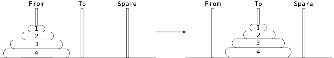
For example, the only two legal moves from the initial position are
For someone not familiar with recursion, this looks like a hard problem. In fact it is easy!
The base case is n=1 and moving a pile of 1 disks from peg From to peg To takes only one turn and doesn't even need peg Spare. In our notation the solution is 1:FT.
Referring to the picture let's do n=4. That is we want to move the 4-3-2-1 pile from peg From to peg To and can use the remaining peg if needed. We denote this goal as 4-3-2-1:FT and note again that the peg not listed (in this case peg Spare) is available for intermediate storage. Solving this 4-disk problem is a three-step solution.
Step 2 is simple enough. After step 1 peg F (From) has only one disk and peg T has none so of course we can move the lone disk from F to T. But steps 1 and 3 look like the another hanoi problem.
Exactly. That's why were done!!
Indeed the solution works for any number of disks. In words the algorithm is: to move a bunch of disks from one peg to another, first, move all but the bottom disk to the remaining (spare) peg, then move the bottom disk to the desired peg, and finally move the all-but-the-bottom pile from the spare to the desired peg.
Show some emacs solutions. The speed can be changed by customizing `hanoi-move-period'.
How many individual steps are required?
Let S(n) be the number of steps needed to solve an n-disk hanoi problem.
Looking at the algorithm we see.
These two equations define what is called a recurrence. In Basic Algorithms (310), you will learn how to solve this and some other (but by no means all) recurrences.
In this class we will be informal. Note that equation 2 says that, if n grows by 1, S(n) nearly doubles.
What function doubles when its argument grows by 1?
Answer: f(n) = 2n
So we suspect the answer to our recurrence will be something like 2n. In fact the answer is S(n)=2n-1.
Let's check S(1)=21-1=2-1=1. Good.
Does S(n)=2S(n-1)+1 as required? We need to evaluate both sides and see.
S(n)=2n-1
2S(n-1)+1 = 2(2n-1-1)+1
= 2n-2+1 = 2n-1
as required.
I feel bound to report that there is another simple solution, one
that does not use recursion.
It is not simple to see that it works and it is not
as elegant
as the recursive solution (at least not to my
eyes).
Do one in class.
  public class Hanoi1 {
  public static void main (String[] args) {
    hanoi(4, 'F', 'T', 'S');
  }
  public static void hanoi(int n, char from,
                        char to, char spare) {
    if (n>0) {
      hanoi(n-1, from, spare, to);
      System.out.println(n + ":" + from + to);
      hanoi(n-1, spare, to, from);
    }
  }
}
On the right is a bare-bones solution. Clearly the main program should read in the value for n instead of hard-wiring 4 and the output is spartan. I did this to show that the algorithm itself really is easy: the hanoi() method just has three lines, directly corresponding to the three lines in the algorithm.
Read.
The book's program accepts input, which it error checks, and invokes its hanoi() method. The latter produces more informative output, which is indented proportional to the current depth of recursion.
Read.
Start Lecture #11
Remark: Lab 3 assigned. The wording on 3B was improved Sunday morning.
Definition: A Graph is a data structure consisting of nodes and edges. An edge is viewed as a line connecting two nodes (occasionally the two nodes are equal and the edge is then often referred to as a loop).
Definition: A graph is called Directed if the each edge has a distinguished start and end. These edges are drawn as arrows to indicate their direction and such directed edges are normally called arcs.
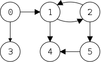
On the right we see a small directed graph. It has 6 nodes and 7 arcs. We wish to determine reachability, that is for each node, we want to know which nodes can be reached by following a path of arcs.
A node, by definition, can reach itself. This can be thought of as following a path of zero arcs.
For example the reachability of the drawn graph is
0: 0 1 2 3 4 5 1: 1 2 4 5 2: 1 2 4 5 3: 3
4: 4 5: 4 5.
One question we must answer is how do we input the graph. We will use what could be called incidence lists. First we input the number of nodes and then, for each node, give the number of nodes directly reachable and a list of those nodes.
For example, the input for the drawn graph is 6 2 1 3 2 2 4 2 1 5 0
0 1 4.
Written in the notation used above for reachability, the given arcs
are
0: 1 3 1: 2 4 2: 1 5 3: 4: 5:
4.
  for each successor
     the successor is reachable
     recurse at this successor
To compute reachability we begin by noting that each node is reachable from itself (as mentioned above) and then apply the algorithm on the right.
Let's say we want to know which nodes are reachable from 2. In the beginning we know only that 2 is reachable from 2. The algorithm begins by looking at the successors of 2, i.e., the destinations of the arcs that start at 2. The first successor we find is 1 so we recursively start looking for the successors of 1 and find 4 (so far the nodes reachable from 2 are 2, 1, and 4).
Then we recursively look for successors of 4. There are none so we have finished looking for the successors of 4 and return to the successors of 1.
There is an infinite loop lurking, do you see it?
The next successor of 1 is 2 so we should now look for successors of 2. But, if we look for successors of 2, will find 1 (and 5) and recursively start looking (again) for successors of 1, then find 2 as a successor of 1, which has 1 as a successor, which ... .
The loop 1 to 2 to 1 to 2 ... is endless. We must do better.
  for each successor
    if the successor is not listed
      list it
      recurse at this successor
The fix is that we do not recurse if we have already placed this node on the list of reachable nodes. On the right we see the pseudocode, with this correction.
Let's apply this pseudocode to find the nodes reachable from 2, remembering that, by definition, 2 is reachable from 2.
The full Java solution is here and I have a handout so that you can read it while something else is on the screen.
This class has two fields:
The constructor is given the number of nodes and creates the fields.
Since the fields have private access, there are methods to set and get various values.
The main program reads input and sets the values in the arcs array. For example, to match our graph the input would be 6 2 1 3 2 2 4 2 1 5 0 0 1 4 as described above. With this input arcs.length==6, arcs[0].length==2, arcs[0,0]==1, arcs[0,1]=3, etc.
The arcs ragged array could be written as follows (the two blank lines represent the fact that there are no arcs leaving nodes 3 and 4).
  1 3
  2 4
  1 5


  4
In class draw the arcs ragged array showing the full Java details.
The two print routines are straightforward; we shall see their output in a few minutes.
CalcReachability() itself does very little.
As indicated, the helper does the real work. It is basically the pseudocode above translated into Java.
One interesting question is, "Where is the base case?".
It is not trivial to find, but it is there! The base case is the case when each successor has already been marked reachable. Note that in this case, the if predicate evaluates to false for each iteration. Thus the method returns without calling itself recursively.
Question: What does this method accomplish,
It doesn't ever return a value?
Answer: It (sometimes) modifies
the reachable parameter.
Question: How can that be an accomplishment since
Java is call-by-value and changes to parameters are not seen by the
caller?
Answer: The usual answer ...
... reference semantics.
Go over execution of the entire program on the input used for the diagram above.
Homework: Draw a directed graph with 7 nodes so that node 1 can reach all nodes and all other nodes can reach only themselves.
For this section we are considering only what are called
singly-linked lists where all the link pointers go in the same
direction.
All our diagrams to date have been of singly-linked lists, but we
will also study doubly-linked lists, which have pointers in both
directions (so called next
and prev
pointers).
If we use a loop to process a (singly-)linked list, we can go only forwards so it becomes awkward when we need to access again a node that we have previously visited.
With recursive calls instead of a loop, we will visit the previous links again when the routines return. Hopefully, the next example with make this clear
Hand out a copies of LLStringNode.java and DemoReversePrint.java, which might not fit conveniently on the screen. These routines can also be found here.
  public class LLStringNode {
      private String info;
      private LLStringNode link = null;

      public LLStringNode(String info) { this.info = info; }

      public String getInfo() { return info; }
      public void setInfo(String info) { this.info = info; }
      public LLStringNode getLink() { return link; }
      public void setLink(LLStringNode link) { this.link = link; }
  }

public class DemoReversePrint {
    public static void main (String[] args) {
        LLStringNode node1 = new LLStringNode("node # 1");
        LLStringNode node2 = new LLStringNode("node # 2");
        LLStringNode node3 = new LLStringNode("node # 3");
        LLStringNode node4 = new LLStringNode("node # 4");

        node1.setLink(node2);
        node2.setLink(node3);
        node3.setLink(node4);

        System.out.println("Printing in original order");
        printFor(node1);
        System.out.println("Printing in reverse order");
        printRev(node1);
        System.out.println("Printing forward recursively");
        printForRec(node1);
    }
    public static void printFor(LLStringNode node) {
        while (node != null) {
            System.out.println("  " + node.getInfo() );
            node = node.getLink();
        }
    }
    public static void printRev(LLStringNode node) {
        if (node.getLink() != null)
            printRev(node.getLink());
        System.out.println ("  " + node.getInfo() );
    }
    public static void printForRec(LLStringNode node) {
        System.out.println ("  " + node.getInfo() );
        if (node.getLink() != null)
            printForRec(node.getLink());
    }
}
LLStringNode.java is quite simple. Each node has two fields, the constructor initializes one and there is a set and get for each.
The main program first creates a four node list
node1-->node2-->node3-->node4 and then prints it three
times.
The first time the usual while loop is employed and the
(data components of the) nodes are printed in the their original
order.
The second time recursion is used to get to the end of the list (without printing) and then printing as the recursion unwinds. Show this in class.
The third time recursion is again used but values are printed as the recursion moves forward not as it unwinds. Show in class that this gives the list in the original order.
  while (node != null)
    push info on stack
    node = node.getLink()
  While (!stack.empty())
    print stack.top()
    stack.pop()
On the right we see pseudocode for a non-recursive, reversing print. As we shall soon see the key to implementing recursion is the clever use of a stack. Recall that an important property of dynamically nested function calls is their stack-like LIFO semantics. If f() calls g() calls h(), then the returns are in the reverse order h() returns, then g() returns, then f() returns.
Consider the recursive situation main calls f() calls f() calls
f().
When the first call occurs we store the information about the f() on
a stack.
When the second call occurs, we again store the information, but now
for the second
f().
Similarly, when the third calls occurs, we store the information for
the third
f().
When this third
f() returns, we pop the stack and have
restored the environment of the second
f().
When this invocation of f() returns, we pop again and have restored
the environment of the original f().
This is shown in more detail just below.
Homework: The printFor() method prints each node once. Write printForN(), which prints the first node once, the second node twice, the third node three times, ..., the Nth node N times.
If f() calls f() calls f() ..., we need to keep track of which f we
are working on.
This is done by using a stack and keeping a chunk of memory
(an activation record
) for each active execution of f().
The first diagram below shows the life history of the activation
stack for an execution of f(2) where f() is the fibonacci function
we saw at the beginning of the chapter.
Below that is the activation stack for f(3).
At all times the system is executing the invocation at the current top of the stack and is ignoring all other invocations.
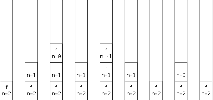
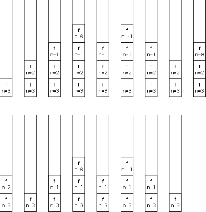
  n = getInput.nextInt();
  double[] x = new double[n];
Some older programming languages (notably old versions of Fortran) did not have recursion and required all array bounds to be constant (so the Java code on the right was not supported). With these some languages the compiler could determine, before execution began where each variable would be located.
This rather rigid policy is termed static storage allocation since the storage used is fixed prior to execution beginning.
In contrast to the above, newer languages like Java support both recursion and arrays with bounds known only during run time. For these languages additional memory must be allocated while execution occurs. This is called dynamic storage allocation.
One example, which we have illustrated above is the activation stack for recursive programs like fibonacci.
There is one case where it is easy to convert a recursive method to an iterative one. A method is called tail-recursive if the only recursion is at the tail (i.e., the end). More formally
Definition: A method f() is tail-recursive if the only (direct or indirect) recursive call in f() is a direct call of f() as the very last action before returning.
The big deal here is that when f() calls f()
and the 2nd f() returns, the first f()
returns immediately thereafter.
Hence we do not have to keep all the activation records
.
  int gcd (int a, int b) {       int gcd (int a, int b) {
                               start:
    if (a == b) return a;          if (a == b) return a;
    if (a > b)                     if (a > b) {
        return gcd(a-b,b);              a = a-b; goto start; }
    return gcd(a,b-a); }           b = b-a; goto start; }
As an example consider the program on the near right. This program computes the greatest common divisor (gcd) of two positive integers. As the name suggests, the gcd is the largest integer that (evenly) divides each of the two given numbers. For example gcd(15,6)==3.
Do gdc(15,6) on the board showing the activation stack.
It is perhaps not clear that this program actually computes the correct value even thought it does work when we try it. We are actually not interested in computing gcd's so let's just say we are interested in the program on the near right and consider it a rumor that it does compute the gcd.
Now look at the program on the far right above. It is not legal Java since Java does not have a goto statement. The (famous/infamous/notorious?) goto simply goes to the indicated label.
Again execute gcd(15,6) and notice that it does the same thing as the recursive version but does not make any function calls and hence does not create a long activation stack.
Remark: Good compilers,
especially those for functional languages
, which make heavy
use of recursion, automatically convert tail recursion to
iteration.
Recursion is a powerful technique that you will encounter frequently in your studies. Notice how easy it made the hanoi program.
It is often useful for linked lists and very often for trees. The reason for the importance with trees is that a tree node has multiple successors so you want to descend from this node several times. You can't simply loop to go down since you need to remember for each level what to do next.
Draw a picture to explain and compare it to the fibonacci activation stack picture above.
Start Lecture #12
Remark: Wording change in honors supplement.
Whereas the stack exhibits LIFO (last-in/first-out) semantics, queues have FIFO (first-in/first-out) semantics. This means that insertions and removals occur at different ends of a queue; whereas, they occur at the same end of a stack.
A good physical example for stacks is the dish stack at hayden; a good physical example for a queue is a line to buy tickets or to be served by a bank teller. In fact in British English such lines are called queues.
Following the example of a ticket line, we call the site where items are inserted the rear of the queue and the site where items are removed the front of the queue.
Personally, I try to reserve the term queue
for the
structure described above.
Some call a stack a LIFO queue (I shudder when I hear that) and
thus call a queue a FIFO queue.
Unfortunately, the term priority queue
is absolutely
standard and refers to a structure that does not have FIFO
semantics.
We will likely discuss priority queues later this semester, but not
in this chapter and never by the simple name queue
.
As with stacks there are two basic operations: insertion and removal. For stacks those are called push and pop; for queues they are normally called enqueue and dequeue.
We have discussed real-world
examples, but queues are very
common in computer systems.
One use is for speed matching. Here is an example from 202 (operating systems). A disk delivers data at a fixed rate determined by the speed of rotation and the density of the bits on the medium. The OS cannot change either the bit density or the rotation rate. If software can't keep up (for example the processor is doing something else), the disk cannot be slowed or stopped. Instead the arriving data must be either saved or discarded (both options are done).
When the choice is to save the data until needed, a queue is used so that the software obtaining the data, gets it in the same order it would have were it receiving the data directly from the disk.
This use of a queue is often called buffering and these queue are often called buffers.
As with stacks, we will distinguish between queues having limited capacity (bounded queues) from those with no such limit (unbounded queues). Following the procedure used for stacks, we give 3 interfaces for queues: the all inclusive QueueInterface, which describes the portion of the interface that is common to both bounded and unbounded queues; BoundedQueueInterface, the extension describing bounded queues; and UnBoundedQueueInterface, the extension for unbounded queues.
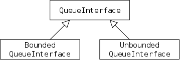
On the right we see the relationship between the three interfaces.
Recall that the arrows with single open triangles
signify extends
.
For example, BoundedQueueInterface extends
QueueInterface.
Below we see a larger diagram covering all the interfaces and classes introduced in this chapter.
  package ch05.queues;
  public interface QueueInterface<T> {
    T dequeue() throws QueueUnderflowException;
    boolean isEmpty();
  }
For any queue we need enqueue and dequeue operations. Note, however, that the enqueue is different for bounded and unbounded queues. A full bounded queue cannot accommodate another element. This cannot not occur for an unbounded queue, which cannot be full. Thus both the isFull() predicate and the enqueue() mutator cannot be specified for an arbitrary queue. As a result only the isEmpty() predicate and the dequeue() mutator are specified.
If the mutator encounters an empty queue, it raises and exception.
  package ch05.queues;
  public interface BoundedQueueInterface<T> {
    void enqueue(T element) throws QueueOverflowException;
    boolean isFull();
  }
For bounded queues we do need an isFull() predicate and the enqueue() method, when encountering a full queue, throws an exception.
  package ch05.queues;
  public interface BoundedQueueInterface<T> {
    void enqueue(T element);
Unbounded queues are simpler to specify. Since they are never full, there is no isFull() predicate and the enqueue() method does not raise an exception.
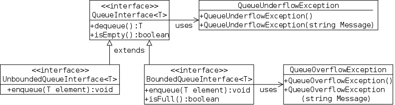
Note the following points that can be seen from the diagram.
underflow.
import ch05.queues.*;
import java.util.Scanner;
public class DemoBoundedQueue {
  public static void main (String[] args) {
    Scanner getInput = new Scanner(System.in);
    String str;
    BoundedQueueInterface<Integer> queue =
      new ArrayBndQueue<Integer>(3);
    while (!(str=getInput.next()).equals("done"))
      if (str.equals("enqueue"))
        queue.enqueue(getInput.nextInt());
      else if (str.equals("dequeue"))
        System.out.println(queue.dequeue());
      else
    System.out.println("Illegal");
  }
}
The example in the book creates a bounded queue of size three; inserts 3 elements; then deletes 3 elements. That's it.
We can do much more with a 3 element queue. We can insert and delete as many elements as we like providing there are never more than three enqueued.
For example, consider the program on the right. It accepts three kinds of input.
An unbounded number of enqueues can occur just as long as there are enough dequeues to prevent more than 3 items in the queue at once.
The Java library has considerably more sophisticated queues than the ones we will implement, so why bother? There are several reasons.
class SomethingOrOtherQueue<T>
All these implementations will be generic so each will have a header line of the form shown on the right, where T is the class of the elements.
For example the ArrayBndQueue<Integer> class will
be an array-based bounded queue of Integer's.Remember
that ArrayBndQueue<float> is illegal.
Why?
Answer float is a primitive type, and a class type
(e.g. Float) is required.
The basic idea is clear: Store the queue in an array and keep track of the indices that correspond to the front and rear of the queue. But there are details.
The book's (reasonable) choice is that the current elements in the queue start at index front and end at index rear. Some minor schenanigans are needed for when the queue has no elements
First we try to mimic the stack approach where one end of the list is at index zero and the other end moves. In particular, the front index is always zero (signifying that the next element to delete is always in slot zero), and the rear index is updated during inserts and deletes so that it always references the slot containing the last item inserted.
The following diagram shows the life history of a ArrayBndQueue<Character> class of size 4 from its creation through four operations, namely three enqueues and one dequeue.
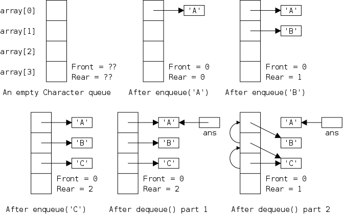
Since the Front of the queue is always zero, we do not need to keep track of it. We do need a rear data field.
Go over the diagram in class, step by step.
Note that the apparent alias in the last frame is not a serious problem since slot number 2 is not part of the queue. If the next operation is an enqueue, the alias will disappear. However, some might consider it safer if the dequeue explicitly set the slot to null.
Homework: Answer the following questions (discuss them in class first)
This queue would be easy to code, let's sketch it out in class.
This queue is simple to understand and easy to program, but is not normally used. Why?
The loop in dequeue() requires about N steps if the currently N elements are enqueued. The technical terminology is that enqueue() is O(1) and dequeue() is O(N).
CircularArrays)
This next design will have O(1) complexity for
both enqueue() and dequeue().
We will see that it has an extra trick
(modular arithmetic)
and needs a little more care.
As mentioned in the very first lecture, we will sometimes give up
some simplicity for increased performance.
The following diagram shows the same history as the previous one, but with an extra dequeue() at the end. Note that now the value of Front changes and thus must be maintained.
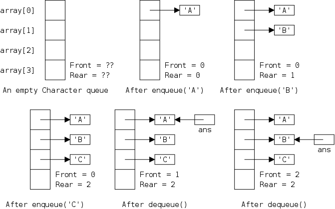
Note first that the last frame represents a queue with only one element. Also note that, similar to the previous diagram, the apparent aliases aren't serious and can be eliminated completely by setting various slots null.
We might appear to be done, both operations are O(1). But, no.
Imagine now three more operations enqueue('D'); dequeue(); enqueue('E'); The number of elements in the queue goes from the current 1, to 2, back to 1, back to 2.
However, it doesn't work because the value of Rear is now 4, which does not represent a slot in the array.
Note that alternating inserts and deletes move both Front and Rear up, which by itself is fine. The trouble is we lose the space below!
That is why we want a circular array so that we consider the slot after 3 to be slot 0. The main change when compared to the previous implementation is that instead of rear++ or ++rear we will use rear=(rear+1)%size
In the fixed-front implementation the number of elements in the queue was Rear+1 so, by maintaining Rear, we were also tracking the current size. That clearly doesn't work here as we can see from the picture just above. However the value Rear+1-Front does seem to work for the picture and would have also worked previously (since then Front was 0).
Nonetheless in the present implementation we will separately track the current size. See the next (optional) section for the reason why.
I will follow the book and explicitly track the number of elements in the queue (adding 1 on enqueues and subtracting 1 on dequeues). This seem redundant as mentioned in the immediately preceding section.
But what happens when Rear wraps around, e.g., when we enqueue two more elements in the last diagram? Rear would go from 2 to 3 to 0 and (Rear-Front)+1 becomes (0-2)+1=-1, which is crazy. There are three elements queued, certainly not -1. However, the queue size is 4 and -1 mod 4 = 3. Indeed (Rear+1-Front) mod Capacity seems to work.
But now comes the real shenanigans about full/empty queues. If you carry out this procedure for a full queue and for an empty queue you will get the same value. Indeed using Front and Rear you can't tell full and empty apart.
One solution is to declare a queue full when the number of elements is one less than the number of slots. The book's solution is to explicitly count the number of elements, which is fine, but I think the subtlety should be mentioned, even if only as a passing remark.
The fixed-front is simpler and does not require tracking the current size. But the O(N) dequeue complexity is a serious disadvantage and I believe the circular queue implementation is more common for that reason.
This class is simple enough that we can get it (close to) right in class ourselves. The goal is that we write the code on the board without looking anywhere. To simplify the job, we will not worry about QueueInterface, BoundedQueueInterface, packages, and CLASSPATH.
You should compare our result with the better code in the book.
We certainly need the queue itself, and the front and rear pointers to tell us where to remove/insert the next item. As mentioned we also need to explicitly track the number of elements currently present. We must determine the correct initial values for front and rear, i.e. what their values should be for an empty queue.
Finally, there is the sad story about declaring and allocating a generic array (an array whose component type is generic).
Although we are not officially implementing the interfaces, we will supply all the methods mentioned, specifically dequeue(), enqueue(), isEmpty(), and is isFull().
I grabbed the main program from the end of section 5.2 (altered it slightly) and stuck it at the end of the class we just developed. The result is here.
In chapter 3 on stacks, after doing a conventional array-based
implementation, we mentioned the Java library
class ArrayList, which implements an
unbounded array
, i.e., an array that grows in size when
needed.
Now, we will implement an unbounded array-base
queue.
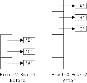
The idea is that an insert into a full queue, increases the size of the underlying array, copies the old data to the new structure, and then proceeds. Specifically, we need to change the following code in ArrayBndQueue. The diagram shows a queue expansion.
Let's do the mods in class. The first step is to figure out enlarge() based on the picture.
The UML diagrams are helpful for writing applications so here is the full one for queues, including linked types we haven't yet studied.
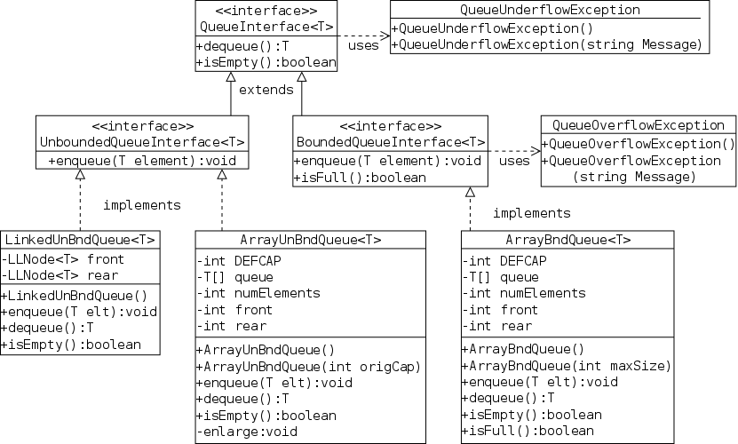
Start Lecture #13
Homework: 1, 2, 6 (these three should have been assigned earlier) 13.
This simple program proceeds as follows. Read in a string and then push (on a stack) and enqueue (on a queue) each element. Finally, pop and dequeue each element. To be a palindrome, the first element popped must match the first element dequeued, the second popped must match the second dequeued, etc.
  public class Palindrome {
    public static boolean isPalindrome(String str) { ... }
  }
Recall that a palindrome reads the same left to right as right to left. Lets write the predicate isPalindrome() using the following procedure.
Note that this is not a great implementation; it is being used just to illustrate the relation between stacks and queues. For a successful match each character in the string is accessed 5 times.
A better program (done in 101!) is to attack the string with charAt() from both ends. This accesses each character only once.
Indeed, if our 102 solution didn't use a queue and just reaccessed the string with charAt() a second time, we would have only 4 accesses instead of 5.
The book's program only considers letters so AB?,BA
would
be a palindrome.
This is just an early if statement to ignore non letters
(the library Character class has an isLetter()
predicate, which does all the work.
Normal I/O and use the palindrome class.
Read.
In this card game you play cards from the top and, if you win
the battle
, you place the won cards at the bottom.
So each player's hand can be modeled as a queue.
main()
  loop N times
    flip a coin
    if heads
       produce()
    else
       consume()

produce()
  if queue is not full
    generate an item
    enqueue the item

consume()
  if queue is not empty
    dequeue an item
    print the item
A very real application of queues is for producer-consumer problems where some processes produce items that other processors consume. To do this properly would require our studying Java threads, a fascinating (but very serious) topic that sadly we will not have time to do.
For a real world example, imagine email. At essentially random times mail arrives and is enqueue. At other essentially random times, the mailbox owner reads messages. (Of course, most mailers permit you to read mail out of order, but ignore that possibility).
We model the producer-consumer problem as shown on the right. This model is simplified from reality. If the queue is full, our produce is a no-op; similarly for an empty queue and consume.
As you will learn in 202, if the queue is
full, all producers are blocked
, that is, the OS stops
executing producers until space becomes available (by a consumer
dequeuing an item).
Similarly, consumers are blocked when the queue is empty and wait
for a producer to enqueue an item.
This is easy. Ask Math.random() for a double between 0 and 1. If the double exceeds 0.5, declare the coin heads. Actually this is flipping a fair coin. By changing the value 0.5 we can change the odds of getting a head.
A simple Java program, using the book's ArrayBndQueue is here.
By varying the capacity of the queue and N, we can see the importance of sufficient size queues. I copied the program and all of .../ch05/queues to i5 so we can demo how changing the probability of heads affects the outcome.
As with linked stacks, we begin linked queues with a detailed diagram showing the result of creating a two node structure, specifically the result of executing.
  UnboundedQueueInterface<Integer> queue = LinkedUnBndQueue<Integer>();
  queue.enqueue(new Integer(10));
  queue.enqueue(20);   // Uses autoboxing
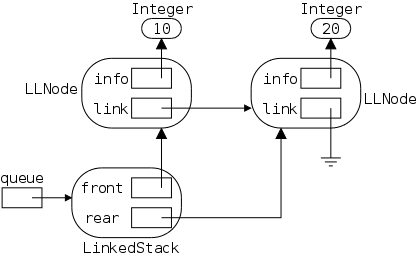
Normally, one does not show all the details we have on the right, especially since some of them depend on Java. A typical picture for this queue is shown below. Given the Java code, you should be able to derive the detailed picture on the right from the simplified picture below.
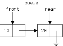
Homework: 30.
The goal is to add a new node at the rear. An unbounded queue is never full, so overflow is not a concern.
Your first thought might be that this is a simple 3-step procedure.
There is a subtle failure lurking here.
Presumably, the current last node
is the one currently
pointed to by rear.
That assertion is correct most, but not all, of the
time, i.e., it is wrong.
The failure occurs when inserting into an empty queue, at which point rear does not point to the last node; instead rear==null.
The fix is to realize that for an initially empty queue we want front (rather than the non-existent last node) to point to the new node.
To motivate this last statement, first imagine inserting into the queue drawn above, which currently contains the Integers 10 and 20. You want the new node to be the successor of (i.e., be pointed to by) the 20-node, which is two nodes after front.
Now imagine a smaller queue with only the 10-node; this time the new node should be the successor of the 10-node, which is one node after front.
  public void enqueue(T data) {
    LLNode<T> newNode = new LLNode<T>(data);
    if (isEmpty())
      front = newNode;
    else
      rear.setLink(newNode);
    rear = newNode;
  }
Now imagine a yet smaller queue with no nodes. By analogy, this time the new node should be the successor of the node zero nodes after front, i.e., it should be the successor of front itself
The resulting method is shown on the right.
The goal is to remove the front node. As with enqueue, dequeue seems simple.
  public T dequeue() {
    if (isEmpty())
      throw new QueueUnderflowException("Helpful msg");
    T ans = front.getInfo();
    front = front.getLink();
    if (front == null)
      rear = null;
    return ans;
  }
Again this works only most of the time, i.e., is wrong.
Clearly we can't dequeue from an empty queue. Instead we raise an exception.
The more subtle concern involves a 1-element queue. In this case front and rear point to the node we are removing. Thus we must remember to set rear=null, as shown in the code on the right.
Since QueueUnderflowException is unchecked, we are not required to include a throws clause in the method header.
  package ch05.queues;
  import support.LLNode;
  public class LinkedUnbndQueue<T>
         implements UnboundedQueueInterface<T> {
    private LLNode<T> front=null, rear=null;
    public boolean isEmpty()    { return front == null; }
    public void enqueue(T data) { // shown above }
    public T dequeue()          { // shown above }
  }
The entire package is on the right. An empty queue has front and rear both null. A nonempty queue has neither null, so isEmpty() is easy.
The implementation on the right uses the generic LLNode class found in the support package.
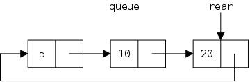
If we are a little clever, we can omit the front pointer. The idea is that, since the link component of the rear node is always null, it conveys no information. Instead of null we store there a pointer to the first node and omit the front data field from the queue itself.
The result, shown on the right, is often called a circular queue. Although it clearly looks circular, one could say that it doesn't look like a queue since it doesn't have two ends. Indeed, from a structural point of view view it has no ends. However, we can write enqueue and dequeue methods that treat the rear as one end and the successor-of-rear (which is the front) as the other end.
An empty queue has rear null and a one element queue has the single node point to itself. Some care is needed when constructing the methods to make sure that they work correctly for such small queues (the so-called boundary cases).
The rough comparison is similar to the stack situation and indeed many other array/linked trade-offs.
With the linked implementation you only allocate as many nodes as you actually use; the unbounded array implementation approximates this behavior; whereas, for the bounded array implementation, you must allocate as many slots as you might use.
However, each node in a linked implementation requires a link field that is not present in either array implementation.
All are fast. The linked enqueue requires the runtime creation of memory, which costs more than simple operations. However, the array constructors requires time O(#slots) since java initializes each slot to null and the unbounded array constructor copies elements.
We run races below.
Read.
The goal is to quantify how fast the queues are in practice. We will compare the two unbounded queues. Since they both implement the same interface we can declare them to be the same type and write one method that accepts either unbounded queue and performs the timing.
There are many possibilities, what I chose was to enqueue N elements and then dequeue them. This set of 2N operations was repeated M times.
The results obtained for N=1,000,000 and M=1,000 were
  An array-based unbounded queue requires 71216 milliseconds
  to enqueue and dequeue 1000000 elements 1000 times.
  A linked-based unbounded queue requires 31643 milliseconds
  to enqueue and dequeue 1000000 elements 1000 times.
So 2 billion operations take about 50 seconds or 40MOPS (Millions of Operations Per Second), which is pretty fast.
Timing events is fairly easy in Java, as usual this is due to the extensive library. For this job, it is the Date class in java.util that performs the heavy lifting.
When you create a date object (using new of course), a field in the object is initialized to represent the current time and this value can be retrieved using the getTime() method.
Specifically, the value returned by getTime() is the number of milliseconds from a fixed time to the time this date object was created. That fixed time happens to be 1 January 1970 00L00:00 GMT, but any fixed time would work.
Therefore, if you subtract the getTime() values for two Date objects, you get the number of milliseconds between their creation times.
Let's write a rough draft in class. My solution is here.
Queues are an important data structure. Their key property is the FIFO behavior exhibited by enqueues and dequeues.
We have seen three implementations, an array-based implementation where each created queue is of a fixed size, and both array-based and linked-based implementations where queue grow in size as needed during execution.
Remark: End of Material on Midterm.
Start Lecture #14
Start Lecture #15
Start Lecture #16
Remarks:
Lists are very common in both real life and computer programs. Software lists come in a number of flavors and the division into subcategories is not standardized.
The book and I believe most authors/programmers use the term list
in a quite general manner.
The Java library, however, restricts a list to be ordered.
The most general list-like interface in the library
is Collection<E>, and the (very extensive)
ensemble of classes and interfaces involved is called the
Collection Framework
.
The library is rather sophisticated and detailed; many of the classes involved implement (or inherit) a significant number of methods. Moreover, the implementations strive for high performance. We shall not be so ambitious.
Differences between various members of the collection include.
We will be defining predicates contains() that determine if a given list contains a given element. For this to make sense, we must know when two elements are equal.
Since we want some lists to be ordered, we must be able to tell if one element is less than another.
We have seen that, for objects, the == operator tests if the references are equal, not if the values in the two objects are equal. That is, o1==o2 means that both o1 and o2 refer to the same objects. Sometimes the semantics of == is just right, but other times we want to know if objects contain the same value.
Recall that the Object class defines an equals() method that has the == semantics. Specifically, o1.equals(2) if and only if both refer to the same value.
Every class is a descendant of object, so equals() is always defined. Many classes, however, override equals() to give it a different meaning. For example, for String's, s1.equals(s2) is true if and only if the two strings themselves are equal (not requiring that the references are equal).
Imagine a Circle class having three fields double r,x,y giving the center of the circle and its radius. We might decide to define equals() for circles to mean that their radii are equal, even though the centers are different. That is, equals() need not mean identical.
  public boolean equals (Circle circle) {
    return this.radius == circle.radius;
  }

  public boolean equals (Object circle) {
    if (circle instanceof Circle)
      return this.radius == ((Circle) circle).radius;
    return false;
  }
The definition of equals() given by Dale is simple, but flawed due to a technical fine point of Java inheritance. The goal is for two circles to be declared equal if they have equal radii. The top code on the right seems to do exactly that.
Unfortunately, the signature of this method differs from the one defined in Object, so the new method only overloads the name equals(). The bottom code does have the same signature as the one in Object, and thus overrides that method.
The result is that in some circumstances, the top code will cause circles to be compared using the equals() defined in Object. The details are in Liang section 11.10 (the 101 text) and in the corresponding section of my 101 lecture notes.
Homework: 1, 2.
To support an ordered list, we need more than equality testing. For unequal items, we need to know which one is smaller. Since I don't know how to tell if one StringLog is smaller than another, I cannot form an ordered list of StringLog's.
As a result, when we define the ArraySortedList<T> class, we will need to determine the smaller of two unequal elements of T. In particular, we cannot construct an ArraySortedList<StringLog>.
Java offers a cryptic header that says what we want.
Specifically, we can write
ArraySortedList<T extends Comparable<T>>
which says that any class plugged in for T must implement
Comparable.
We shall soon see that implementing Comparable means that
we can tell which of two unequal elements is smaller.
Slightly more general and even more cryptic is
the header
ArraySortedList<T extends Comparable<? super T>>
I hope we will not need to use this.
Many classes define a compareTo() instance method taking one argument from the same class and returning an int. We say that x is smaller than y if x.compareTo(y)<0 and say that x is greater than y is x.compareTo(y)>0. Finally, it is normally true (and always for us) that x.compareTo(y)==0 if x.equals(y).
The Java library defines a Comparable interface, which includes just one method, compareTo(), as described above. Hence a class C implements Comparable if C defines compareTo() as desired. For such classes, we can decide which of two unequal members is smaller and thus these are exactly the classes T for which ArraySortedList<T> can be used.
More precisely, recent Java implementations (those with generics) define the Comparable<T> interface, where T specifies the class of objects that the given object can be compared to.
An example may help.
Many library classes (e.g., String)
implement Comparable<T>, where T is the
class itself.
Specifically the header for String states that
String implements
Comparable<String>
This header says that
the String instance method compareTo() takes
a String argument.
Since String does implement Comparable (more precisely Comparable<String>), we can define ArraySortedList<String>.
StringLog does not implement Comparable at all; so we cannot write ArraySortedList<StringLog>.
Homework: 6.
As mentioned above the exact definition of list is not standardized. We shall follow the book's usage. One property of our lists is that each non-empty list has a unique first element and a unique last element (in a 1-element list the first and last elements are the same). Moreover the elements in a non-empty list have a linear relationship.
Definition: A set of elements has a Linear Relationship if each element except the first has a unique predecessor and each element except the last has a unique successor.
Lists can be
These assumptions are straight from the book
current position, the position of the next element accessed by getNext(). This position is incremented by getNext(), zeroed by reset(), and unchanged otherwise.
Start Lecture #17
We see below on the right the two interfaces for lists. The top interface applies to all lists, the bottom gives the additional methods available when the list is indexed.
In both cases elements are equivalent
if
the equals() method in T says so.
As always, when we say that such and such an object is returned, we mean that a reference to the object is returned
Just a few comments are needed as many of the methods are self-explanatory. The exception is the pair reset()/getNext(), which is discussed in a separate section by itself.
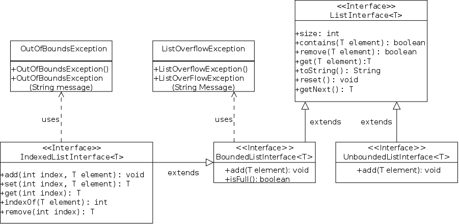
nicely formattedrepresentation of the list.
In an indexed list elements can be referred to by index (as in an array, a good model for such lists). Legal values for the index are 0..size()-1. All methods accepting an index throw an IndexOutOfBoundsException if given an illegal value.
Since elements have a linear relationship, it makes sense to talk of looping over the list from the first element to the last. The Java library has a super-slick and somewhat complicated mechanism to do this in an elegant manor (see the Iterable<T> interface, for details). We follow the book and define the following modest looping procedure.
All our List implementations keep track of the
current position
of the list.
  list.reset()
  for (int i=0; i<list.size(); i++) {
    element = list.getNext();
    // play with element
  }
The code on the right shows a typical usage of these methods for a List named list. We use size() to iterate the correct number of times and use getNext() to advance to the next element.
As is often the case there are some technical details to mention. The easy detail is that, if getNext() is called when at the end of the list, the current position becomes the first element.
More interesting is what to do about empty lists and what happens
if we modify the list while playing with an element
.
Our solution is basically to say Don't do that!
.
The library permits some modifications, but for those not
permitted it also says Don't do that!
.
The requirements are that whenever list.getNext() is
called.
  import ch06.lists.*;
  public class ListExamples {
    public static void main (String[] args) {
      ListInterface<String> list1 =
        new ArrayUnsortedList<String>(3);
      list1.add("Wirth");
      list1.add("Dykstra");
      list1.add("DePasquale");
      list1.add("Dahl");
      list1.add("Nygaard");
      list1.remove("DePasquale");
      System.out.print("Unsorted ");
      System.out.println(list1);

      ListInterface<String> list2 =
        new ArraySortedList<String>(3);
      list2.add("Wirth");
      list2.add("Dykstra");
      list2.add("DePasquale");
      list2.add("Dahl");
      list2.add("Nygaard");
      list2.remove("DePasquale");
      System.out.print("Sorted ");
      System.out.println(list2);

      IndexedListInterface<String> list3 =
        new ArrayIndexedList<String>(3);
      list3.add("Wirth");
      list3.add("Dykstra");
      list3.add("DePasquale");
      list3.add("Dahl");
      list3.add("Nygaard");
      list3.remove("DePasquale");
      System.out.print("Indexed ");
      System.out.println(list3);
    }
  }
This example, which I have taken from the book, illustrates well some differences between the three array-based implementations that we shall study. The first two ArrayUnsortedList and ArraySortedList each implement List; whereas, the third ArrayIndexedList implements IndexedList.
The main method has three sections, one for each list type. In all three cases the same 5 elements are added in the same order and the same element is is removed. The printed results, however, are different for the three cases. Not surprisingly the toPrint() in ArrayIndexedList includes index numbers, while the others do not.
The first surprise is that the output for ArrayUnsortedList does not print the items in the order they were inserted. This is due to the implementation of remove(). The example shown removes the third of the five previously entered elements. Naturally we don't want to leave a hole in slot three.
A natural solution would be to slide each element up so the old fourth becomes the third and the old fifth becomes the fourth. The problem with this solution is that if the first of N elements is deleted you would need to slide N-1 elements, which is O(N) work.
The chosen solution is to simply move the last element into the vacated slot. Remember that an unsorted list has no prescribed order of the elements.
The sorted list, list2, keeps the elements in sorted order. For Java String's the order is lexicographical. Consequently, removal does involve sliding up the elements below the one removed.
Finally, the ArrayIndexedList does not generate sorted lists so is again free to use the faster removal method. As mentioned above, this method enhances the output by generating a string version of the indices.
The result of these decisions is the output below, where I have reformatted the output into three columns so that more can be viewed on the screen
Unsorted List:     Sorted List:       Indexed List:
  Wirth          Dahl         [0] Wirth
  Dykstra        Dykstra          [1] Dykstra
  Nygaard        Nygaard          [2] Nygaard
  Dahl           Wirth        [3] Dahl
Homework: 13, 15.
A UML diagram for all the lists in this chapter is here.
The basic idea for an array-based list is simple: Keep the elements in array slots 0..(size-1), when there are size elements present. We increase size on inserts and deleted it on removals.
We shall meet a new visibility modifier in this section. The reason we can't make do with public and private is that we will be implementing two classes, one derived from the other. In this situation we want to give the derived class access to what would otherwise be private fields and methods of the base class.
More details will be given later when we implement the derived class.
  package ch06.lists;
  public ArrayUnsortedList<T> implements ListInterface<T> {
    protect final int DEFCAP = 100;
    protected T[] list;
    protected int numElements = 0;
    protected int location;
    protected int currentPos;

    public ArrayUnsortedList() { list = (T[]) new Object[DEFCAP]; }
    public ArrayUnsortedList(int origCap) {
      list = (T[]) new Object[origCap];
    }
Most of the code on the right is quite clear. For now, treat protected as private; the fields are not available to ordinary users of the class.
currentPos is use by the reset()/getNext() pair shown below.
Recall that a weakness in Java generics forbids the creation of a generic array, which explains the treatment of list.
Several of the public methods need to search for a given element. This task is given to an helper boolean method find() which, if the element is found, sets location for use by the public methods.
  protected void enlarge() {
    T[] larger = (T[]) new Object[2*list.length];
    for (int i=0; i<numElements; i++)
      larger[i] = list[i];
    list = larger;
  }

  protected boolean find(T target); {
    for (location=0; location<numElements; location++)
      if (list[location].equals(target))
        return true;
    return false;
  }
There are two helper methods.
The enlarge() method is called when an addition is
attempted on a currently full
list.
Recall that all the lists is this chapter are unbounded so
technically are never full.
Unlike the authors who raise the capacity by a fixed amount, I double it.
Then the current values are copied in.
The find() method implements a standard linear search. The only point to note is that the index used is a field and thus available to the public methods that call find().
The authors define a void find() and define a field (found) to hold the status of the search. I prefer a boolean find().
  public void add(T element) {
    if (numElements == list.length)
      enlarge();
    list[numElements++] = element;

  public boolean remove(T element) {
    if (!find(element))
      return false;
    list[location] = list[--numElements];
    list[numElements] = null;
    return true;
  }

  public int size() { return numElements; }

  public boolean contains(T element) {
    return find(element);
  }

  public T get(T element) {
    if (find(element))
      return list[location]
    return null;
  }

  public String toString() {
    String str = "List:\n";
    for (int i=0; i<numElements; i++)
      str = str + " " + list[i] + "\n";
    return str;
  }
The add() method works as expected. For an unsorted list, we are free to add the new element anywhere we wish. It is easiest to add it at the end, so we do so.
Since our lists are unbounded, we must enlarge() the array if necessary.
The remove() method uses find() to determine if the desired element is present and if so where it is located (recall that find() sets location).
Removes can occur at any slot and we cannot leave a hole in the middle. Again we take the easy way out and simply move the last element into the hole.
Does this work if the element was found in highest array
slot?
Answer: Let's try it in class.
The size() method is trivial.
The contains() method is easy given the helper find().
The get() method, like remove() uses find() to determine the location of the desired element, which get() then returns. If find() reports that the element is not present, get() returns null as per its specification.
The toString() method, constructs its return value one line at a time, beginning with a header line and then one line for each listed element.
  public void reset() { currentPos = 0; }

  public T getNext() {
    T next = list[currentPos++];
    if (++currentPos == numElements)
      currentPos = 0;
    return next;
  }
As mentioned previously reset() and getNext() are use to enable looping through a the elements of the list. The idea is that currentPos indicates the next site to access and that getNext() does the access.
The reset() method initializes the loop
by
setting currentPos to zero.
These methods are easy because we forbid the user to mess up the list and do not check whether they do.
Now we want to keep the listed items in sorted order. But this might not even make sense!
I certainly understand a sorted list of Integer's or a sorted list of String's. But a sorted list of blueprints? Or bookcases?
That is, a sorted list of T's makes sense for some T's, but not for others. Specifically, we need that the objects in T can be compared to determine which one comes first.
Java has exactly this concept; it is the Comparable interface. So, we want to require that T implements this interface, which leads to two questions.
  public class ArraySortedList<T>
         implements ListInterface<T>
Our first attempt at a header line for the ArraySortedList class, before considering Comparable but remembering that the class must implement ListInterface<T>, would be something like we see on the right.
  public class ArraySortedList<T implements Comparable>
         implements ListInterface<T>

  public class ArraySortedList<T extends Comparable>
         implements ListInterface<T>
When trying to add the restriction that T implement Comparable, my first guess would be the top header on the right. However, that header is wrong; instead of implements we use the keyword extends, which gives the correct bottom header line. I am not certain of the reason for this choice of keyword, but an indication is below.
This last header is legal Java and illustrates how one limits the classes that can be plugged in for T. It is not perfect, however. We shall improve it after first learning how to use Comparable and thereby answering our second question above.
Objects in a class implementing the Comparable interface are ordered. Given two unequal objects, one is less than the other. This interface specifies only one instance method, compareTo(), which has one parameter and returns an int result.
The invocation x.compareTo(y) returns a negative integer, zero, or a positive integer to signify that x is less than, equal to, or greater than y.
The description just above, which did not
mention T, would have been applicable a few years ago and
probably still works
today.
However, modern, generics aware, Java specifies a
generic Comparable<T> interface.
On the right we see proper specifications of classes implementing Comparable.
  public class C implements Comparable<C>

  public class String implements Comparable<String>

  public class C implements Comparable<D>
The first line asserts that an object in C can be compared
to another object in C.
The second line shows (part of) the header line for the familiar
class String.
The third line asserts that an object in C can be
compared to an object in D.
  public class ArraySortedList<T extends Comparable<T>>
         implements ListInterface<T>
On the right we see a proper header for ArraySortedList<T> specifying that the class parameter T must implement Comparable<T>.
In fact the best
header we could write
for ArraySortedList would be
ArraySortedList<T extends Comparable<? super T>> implements ListInterface<T>
What this cryptic header is saying is
that instead of requiring that elements
of T can be compared with other
elements of T, we require that
elements of T can be compared with
elements of some superclass of T.
The ? in the header is
a wildcard
.
Note that T itself is considered a
superclass of T.
Since T extends a superclass
of T, perhaps this explains the choice
of the keyword extends above.
Why all this fuss about Comparable and fancy headings? We must do something since we need to keep the entries of our sorted list ordered. In particular, the add() method must place the new entry in the correct location (and slide the rest down).
The book uses the very first ArraySortedList header line that we considered. Recall that this header did not mention Comparable at all. What gain do we get for our efforts?
  public class ArraySortedList<T>
         implements ListInterface<T>

  public class ArraySortedList<T extends Comparable<T>>
         implements ListInterface<T>
For convenience, both headers are repeated on the right.
Since the first header does not mention Comparable, a simple use of compareTo() for elements would fail to compile since there is no reason to believe that T contains such a method. Hence to find the correct location for add() to place the new element, the book compares this new element with existing elements using the following if statement
if (((Comparable)listElement).compareTo(element) < 0) // list element < add element
I would rate this if statement as roughly equal to our header on the ugliness scale, so using our header to simplify the if statement would be only a wash, not an improvement.
The real advantage of our approach is that the ugly if statement generates a warning from the compiler that it cannot guarantee that the listElement object contains a compareTo() method. This warning is quite appropriate since there is nothing to suggest that listElement, a member of T, is comparable to anything.
With our header the if statement becomes the expected
if (listElement.compareTo(element) < 0) // list element < add element
and, more significantly, generates no warning. As a result we cannot get a runtime error due to an inappropriate class being substituted for T.
We are now in a position to implement ArraySortedList<T> and could do so directly. However, we notice that the only methods that change between ArraySortedList<T> and ArrayUnsortedList<T> are add() (we need to insert the new item in the right place) and remove() (we must slide elements up instead of just placing the last element in the vacated slot). It seems a little silly to rewrite all the other methods so we choose to implement ArraySortedList<T> as an extension of ArrayUnsortedList<T>.
  public class ArraySortedList<T extends Comparable<T>>
    extends ArrayUnsortedList<T> implements ListInterface<T> {
    ArraySortedList()            { super(); }
    ArraySortedList(int origCap) { super(origCap); }

    public void add(T element) {
      int location;
      if (numElements == list.length)
        enlarge();
      for (location=0; location<numElements; location++)
        if ((list[location]).compareTo(element) >= 0)
          break;
      for (int index=numElements; index>location; index--)
        list[index] = list[index-1];
      list[location] = element;
      numElements++;
    }

    public boolean remove(T element) {
      boolean found = find(element);
      if (found) {
        for (int i=location; i<=numElements-2; i++)
          list[i] = list[i+1];
        list[--numElements] = null;
      return found;
    }
  }
The header is a mouthful and conveys considerable information: this generic class requires the argument class to support comparison, inherits from the unsorted list, and satisfies the list specification. The constructors are the same as for the parent (ArrayUnsortedList<T>).
Since this is an unbounded implementation, we first enlarge the list if it is filled to capacity. Next we determine the correct location to use, which is the first location whose occupant is greater than or equal to the new element. To make room for the new element, we shift the existing elements from here on. Finally, we insert the new element and increase the count.
Since we must maintain the ordering, remove is simple. If the item is found, shift down all element from the found location on (thus overwriting the item) and reduce the count. Finally, return whether the item was present.
by Copyor
by Reference
Our list (and stack, and queue) implementations, when given an
element to insert, place (a reference to) the actual object on the
list.
This implementation is referred to as by reference
and, I
believe, is normally desirable.
But putting (a reference to) the actual object on the list can break the list's semantics since this listed object can be changed by the user. For example, the items in ArraySortedList<Integer> can become out of order, if a listed Integer is changed.
This problem can be avoided by having the add() method
make a copy of the item and then insert (a reference to) this
private copy rather than the user-accessible original.
This implementation is referred to as by copy
and requires
extra computation and extra memory when compared to by
reference
.
This extended class supports indexed references. In a sense it permits the user to treat the list as intelligent arrays. The two extensions to ArrayUnsortedList<T> class is to give an additional (indexed based) signatures to existing methods and introduce methods that require indices.
For example, in addition to add(T element), which just promises to add the element somewhere, the indexed list introduces add(int index, T element), which adds the element at the specified index.
New methods such as set(), which updates a specified location, have no analogue without indices.
The methods including an index parameter check the parameters for legality and throw a standard IndexOutOfBoundsException exception if needed.
  package ch06.lists;
  public class ArrayIndexedList<T> extends ArrayUnsortedList<T>
         implements IndexedListInterface<T> {
    public ArrayIndexList()            { super();      }
    public ArrayIndexList(int origCap) {super(origCap); }

    public void add(int index, T element) {
      if ((index<0) || (index>numElements))
         throw new IndexOutOfBounds Exception("Helpful message.");
      if (numElements == list.length)
        enlarge();
      for (int i=numElements; i>index; i--)
        list[i] = list[i-1];
      list[index] = element;
      numElements++
    }

  public T set(int index, T element) {
    if ((index<0) || (index>numElements))
       throw new IndexOutOfBounds Exception("Helpful message.");
    T hold = list[index];
    list[index] = element;
    return hold;
  }

  public int indexOf(T element) {
    if (find(element))
      return location;
    return -1;
  }

  public T remove (int index) {
    if ((index<0) || (index>numElements))
       throw new IndexOutOfBounds Exception("Helpful message.");
    T hold = list[index];
    for (int i=index; i<(numElements-1); i++)
      list[i] = list[i-1];
    list[numElements--] = null;
    return hold;

  public String toString() {
    String str = :List:\n";
    for (int i=0; i<numElements; i++)
      str = str + "[" + i "] " + list[i] + "\n";
    return str;
No surprises here. The list is not sorted so doesn't involve Comparable
After checking the index for legality, the method enlarges the array if necessary.
Since the goal is to place the new element in a specified slot, add() next shifts down the existing elements from the desired slot on. Note that this loop runs backwards.
This method sets the specified slot to the given element and returns the former occupant. The code is straightforward
This simple method returns the index of a sought for element or -1 if the element is not on the list.
This method removes and returns the element in a specified slot. The code is again straightforward.
The only difference between this method and one being overridden is the addition of the index value within brackets.
Homework: 18, 21.
Start Lecture #18
Remarks: I used the following procedure for computing midterm grades.
For *MIDTERM* grades, I do not give + or -.
I certainly do give + and - for final grades.

1.  Normal case:  Midterm exam and labs 1 and 2:
    * Lab average Lavg = (L1+L2)/2
    * Overall average Avg = (2*midExam + Lavg)/3
    * A=90-100  B=80-89  C=70-79  D=60-69  F=0-59

2.  No midterm exam
    * Grade is UE (unable to evaluate)

3.  Midterm exam but only 1 or 0 labs
    * Avg = midExam - 10 (hoping that late labs will appear;
                          for final grades missing labs count as 0!)
    * Same letter grade ranges as case 1
    * Exception.  Missing labs do not lower D to F (I don't fail anyone
      who passes all exams)
Lab 4 had confusing words for a few days so I am extending the due date until 17 November 2012.
Read.
A crucial advantage of sorted lists is that searching is faster. No one would use a telephone directory with the names unsorted.
The linear search algorithm, which we have already seen, is given a list and a desired value. The algorithm can be described as follows.
We can improve this algorithm (a little) by recognizing that if the current list value exceeds the desired value, the desired value is not present. That is the algorithm becomes the following (assuming the list is sorted in ascending order).
In comparison, the binary search algorithm can be described as follows (again assuming the list is sorted in ascending order).
halfof the list; otherwise, search only the lower
half.
My presentation differs in three small ways from the book's.
Since our goal is to write a drop-in replacement for the find() method in ArraySortedList<T>, our header line must be the same as the one we are replacing. Recall that the value returned by find() indicates whether the search was successful. If successful the location instance data field is set. Our replacement must have the same semantics.
protected boolean find(T target)
The required header is shown on the right. (In fact there is no find() method in the code for ArraySortedList<T>; instead it is inherited from ArrayUnsortedList<T>).
The original (linear search) find() searched the entire occupied portion of the array; whereas the binary search algorithm searches smaller and smaller sub-arrays with each recursive call. Thus, we shall need to specify the current lower and upper bounds for the search.
  protected boolean find(T target) {
    return find1(target, 0, numElements-1);
  }
Hence we will need a helper method find1() that accepts these extra parameters and performs the real search. The find() method itself is the trivial routine on the right. It simply passes the job onto find1() telling it to search the entire range of possible values.
  private boolean find1(T target, int lo, int hi) {
    if (lo > hi)
      return false;
    int location = (lo + hi) / 2;
    if (list[location].compareTo(target) == 0)
      return true;
    if (list[location].compareTo(target) < 0)
      return find1(target, location+1, hi);
    return find1(target, lo, location-1);
  }
Perhaps the only subtlety in this method is the first base case, which is represented by the first if statement on the right. When we have reduced the range of interest to the empty set, the item is definitely not present.
The rest of the method is essentially an English-to-Java
translation of the words above describing the algorithm.
If the middle location contains the target, we are done; if it is
less search the upper half
; otherwise search the lower
half
.
Notice that find1() is tail-recursive, that is the two
recursive calls are each the last statement executed.
Question: How can two different calls each be the
last statement?
Answer: Last doesn't mean the last one written, it
means the last one executed.
As we noted before, tail recursive methods can be converted to iterative form fairly easily.
  protected boolean find(T target) {
    int lo=0,  hi=numElements-1;
    while (lo <= hi) {
      location = (lo + hi) / 2;
      if (list[location].compareTo(target) == 0)
        return true;
      if (list[location].compartTo(tartet))
        lo=location+1;
      else
        hi=location-1;
    }
    return false;
  }
In fact the code on the right is essentially the same as the pair above it.
The difference is that instead of a recursive call we just go back to the beginning. The jumping to the beginning and a recursive call start out the same. But when the recursion ends, we normally have more to do in the caller. However, this is tail-recursion so there is nothing more to do.
Lets go through a few searches and see.
How much effort is required to search a list with N items?
For linear search the analysis is easy, but the result is bad.
If we are lucky, the element is found on the first check. If we are unlucky, the element is found at the end of the list or not at all. In these bad cases we check all N list elements. So the best case complexity of linear search is O(1) and the worst case complexity is O(N).
On the average we will find the element (assuming it is present) in the middle of the list with complexity O(N/2)=O(N).
The worst case is still O(N). For example consider searching for an element larger than every listed element.
In binary search, each update of lo or hi reduces the range of interest to no more than half what it was previously. This occurs each iteration or each recursive call, which leads to two questions.
The first question is easy, each iteration and each recursive call, does an amount of work bounded independent of N. So each iteration or recursive call is O(1).
The second question might be easier looked at in reverse. How many times must you multiply 2 by itself to reach at least N? That number is log2(N), which we write as simply log(N) since, by default, in this class logs are base 2. Hence the complexity is O(log(N)), a big improvement. Remember that log(1,000,000,000)<30.
Homework: 42.
We now give linked implementations of both unsorted and sorted
lists.
However, we do not implement a linked, indexed list (even though we
could).
Why not?
Answer: Accessing the linked item at
index i requires traversing the list.
Thus the operation has complexity O(N) where O(N)
is the current size of the list.
This answer illustrates a strong advantage of array-based lists, to balance against the disadvantage of having to enlarge() them or deal with them being full.
As with stacks and queues, reference based lists use the LLNode<T> class.
The UML for all our lists is here. (References to all UMLs are repeated at the end of the notes.)
The authors choose to say Ref rather than Linked since the latter is used by the standard Java library.
  package ch06.lists;
  import support.LLNode;
  public class RefUnsortedList<T> implements ListInterface<T> {
    protected int numElements = 0;
    protected LLNode<T> currentPos = null;
    protected LLNode<T> location;
    protected LLNode<T> previous;
    protected LLNode<T> list = null;
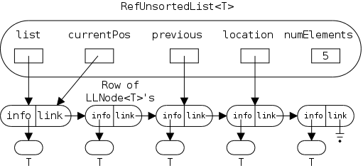
As with the array-based implementation we use an ugly header to avoid an ugly and unsafe if statement found in the book.
The currentPos field is used with the reset()/getNext() pair describe below.
We shall see that removing an item from a given location requires referencing the previous location as well.
Finally, list references the first node on the list (or is null if the list is empty).
These fields are illustrated in the diagram on the right, which shows a list with 5 elements ready for the next-to-last to be remove()'d. reset() has been called so getNext() would begin with the first node (assuming the remove() did not occur).
The default no-arg constructor suffices so no constructor is written.
Homework: 47a, 47b (use the diagram style used on the midterm), 50.
  public void add(T element) {
    LLNode<T> newNode = new LLNode<T>(element);
    newNode.setLink(list); // new  becomes first
    list = newNode;
    numElements++;
  }
Since the list is not sorted we can add elements wherever it is
most convenient and for a single linked list, that is at the front
(i.e., right after
the RefUnsortedList<T>
node itself).
public int size() { return numElements; }
Since we explicitly maintain a count of the number of elements currently residing on the list, size() is trivial.
  public boolean contains(T element) {
    return find(element);
  }

  protected boolean find(T target) {
    location = list;
    while (location != null)
      if (location.getInfo().equals(target))
        return true
      previous = location;
      location = location.getLink();
    return false;
  }
As in the array-based implementations we use a predicate find() instead of a found data field.
You may notice that extra work is performed while searching for an element. This is done so that, after find() is executed the found element is ready for removal.
Note the efficient technique used to determine the actual location and its predecessor (the latter is needed for removal). Thus the superfluous work just mentioned is small.
The workhorse find() is protected so that derived classes (in particular, RefSortedList, to be studied next) can use it.
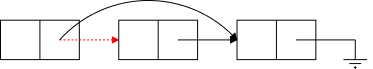
The natural technique to remove a target element from a linked list is to make the element before the target point to the element after the target.
This is shown on the right, where the middle node is the target.
  public boolean remove(T element) {
    boolean found = find(element);
    if (found) {
      if (location = list) // first element
        list = location.getLink();
      else
        previous.setlink(location.getLink());
      numElements--;
    }
    return found;
  }
The only tricky part occurs when the target is first element since there is then is no element before the target. The solution in this case depends on the details of the implementation.
In our implementation, the list field acts as the (link component of the) element before the first element. Hence, the code on the right makes list point at the element after the target when target is the first element.
Start Lecture #19
Remark: The RefUnsortedList<T> header does not need to mention Comparable as I guessed last time. It is fixed now.
  public T get(T element) {
    if find(element)
      return location.getInfo();
    else
      return null;
  }
Whereas the contains() predicate merely determines whether a given element can be found on the list, get() actually returns a reference to the element. As expected, find() again does all the work.
The only question is what to do if the element cannot be found; we specify that null be returned in that case.
  public void reset() { currentPos = list; }

  public T getNext() {
    T next = currentPos.getInfo();
    if (currentPos.getLink() == null)
      currentPos = list;
    else
      currentPos = currentPos.getLink();
    return next;
  }
} // end of class RefUnsortedList<T>
To employ this pair, the user calls reset() to get started and then calls getNext() repeatedly to retrieve successive elements on the list.
It is not hard to think of difficult cases to implement and hence the code on the right seems surprisingly simple. The simplicity is due to the difficult cases being outlawed and not checked for. For example, an empty list gives a null pointer exception when getNext() executes it first instruction.
Specifically, the implementation assumes that when getNext() is invoked:
We shall see next chapter that reset()/getNext() can be applied to some structures that are not lists (we will do binary trees).
There is not much difference between the RefUnsortedList<T> and RefSortedList<T> classes; almost all the methods remain the same. For this reason, we implement the latter as an extension of the former.
One difference between the classes is that now that we want the elements to be in order, we must require that T implement Comparable<T>.
  public class RefSortedList<T extends Comparable<T>>
         extends RefUnsortedList<T>
         implements ListInterface<T> {
The header shows the dependence on RefUnsortedList<T>. There are no fields beyond those of the base class and again the default no-arg constructor suffices. Note that this constructor invokes the superclass constructor.
The one method we do need to change is add(). Previously we chose to insert the new element at the beginning of the list because that was the easiest place. Now we must skip over all existing elements that are smaller than the one we are inserting.
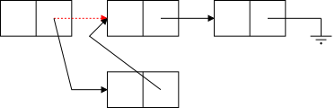
Once we have found the correct location, the insertion proceeds as illustrated on the right. The new node, shown on the bottom row, is to be inserted between the first two nodes on the top row. These nodes are called prevLoc and location in the code below. The former is the last node we skipped over in seeking the insertion site and the latter is thus the first node not skipped.
  public void add(T element) {
    LLNode<T> prevLoc  = null;
    LLNode<T> location = list;
    while (location!=null &&
           location.getInfo().compareTo(element)<0) {
      prevLoc = location;
      location = location.getLink();
    }
    LLNode<T> newNode = new LLNoDE<T>(element);
    if (prevLoc == null) {   // add at front of list
      newNode.setLink(list);
      list = newNode;
    } else {                 // add elsewhere
      newNode.setLink(location);
      prevLoc.setLink(newNode);
    }
    numElements++;
  }
} // end of class RefSortedList<T>
The method begins with a short but clever search loop to find the
two nodes between which the new node is to be inserted.
This loop is similar to the one in find() and deserves
careful study.
Questions How
come .getInfo() does not ever raise
a nullPointerException.
How come location.getInfo() will have
a compareTo() method defined.
Answers: Short circuit evaluation
of &&.
T implements Comparable<T>.
After the loop, we create and insert the new node. The then arm is for insertion at the beginning (done identically to the method in RefUnsortedList<T>); the else arm is for insertion between preLoc and Location.
Finally, we increase the count of elements.
Homework: 47c, 47d, 48.
For practice in the programming technique just illustrated, let's do on the board the problem of finding the second largest element in an array of int's.
A solution is here.
Previously we have studied stacks, a linear structure in which all activity occurs at one end (the top), and queue another linear structure, in which activity occurs at both ends (the front and rear). In this chapter we studied lists, general linear structures in which activity can occur throughout.
We also encountered our first high performance algorithm, binary search, which improves complexity from O(N) for naive searching down to O(logN).
If we use an array-based list, we can employ binary search, which speeds up retrieval from O(N) to O(logN)). However, these lists are not as convenient when the list size is static.
We shall see that binary search trees combine the advantages of O(logN) searching with linked-like memory management.
A key characteristic of lists is their linear structure: Each node (except for the first and last) has a unique predecessor and a unique successor.
Tree nodes, in contrast, have (zero or more) children and (zero or one) parents. As in biology, if A is a child of B, then B is the parent of A. Most nodes do have a parent; the one exception is the tree root, which has no parent. The root can be reached from any other node by repeated moving to the parent.
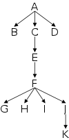
Nodes that have no children are called leaves of the tree. Other nodes are called interior.
We see two small trees on the right.
Note that there is a specific direction inherent in a tree diagram, from root to leaves. In the bottom diagram the direction is shown explicitly with arrowheads; in the top diagram it is implicitly going from top to bottom.
Trees are often used to represent hierarchies.
For example this chapter can be viewed as tree.
The root is Chapter 8 Binary Search Trees
.
This root has 11 children 8.1 Trees
... 8.10
Case Study: Word Frequency Generator
, Summary
.
The node 8.2 The Logical Level
has two children
Tree Elements
and The Binary Search Tree Specification
.
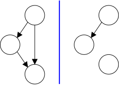
In fact this chapter can be considered as a subtree of the entire
tree of the book.
That bigger tree has as root
Object-Oriented Data Structures Using Java
.
Each chapter
heading is a child of this root and each chapter itself is a subtree
of the big tree.
The two diagrams on the right show graphs that are not trees. The graph on the near right is not a tree since the bottom node has two parents. The graph on the far right, does not have a single root from which all nodes are descendants.
We often think of the tree as divided into horizontal levels. The root is at level 0, and the children of a level n node are at level n+1.
Some authors, but not ours, also use the term depth as a synonym for level.
Unlike level (and depth) which are defined from the root down, height is defined from leaves up. The height of a leaf is 0 and the height of an interior node is one plus the maximum height of its children.
The height of a tree is the height of its root, which equals the maximum level of a node.
For any node A, the subtree (rooted) at A consists of A plus A's children, plus their children, plus their children, ... .
The nodes constituting the subtree at A excluding A itself are called the descendants of A.
If a node X is a descendant of Y, we also say that Y is an ancestor of X.
Two nodes with the same parent are called siblings
Illustrate all these definitions on the board
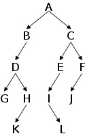
Trees are quite useful in general. However, in this course, we will mostly use trees to speed-up searches and will emphasize a subclass of trees, binary search trees (other trees are used for searching, but we will not be studying them).
Definition: A binary tree is a tree in which no node has more than two children
For example the tree on the right is a binary tree.
We distinguish the right and left child of a node. For example the node H on the right has only a left child, the node I has only a right child, and the root has both a left and right child.
We also talk of the right and left subtrees of a node. The right subtree is the subtree rooted at the right child (assuming the node has a right child; otherwise the right subtree is empty) and similarly for the left subtree.
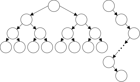
We will see that most of our operations will go up and down trees once or a few times and will not normally move from sibling to sibling. Thus these operations will take time proportional to the height and therefore low-height binary trees are preferable.
Consider all possible binary trees with 15 nodes. What are the maximum and minimum possible heights?
The max is pretty easy: a line. That is 14 nodes with one child and one leaf at the end. These trees have height 14.
The min is not too hard either. We want as many nodes as possible with 2 children so that the tree will be wide, not high. In particular, the minimum height tree has 7 interior nodes (each with 2 children) on the top three levels and 8 leaves on level 3. Its height is 3.
The same reasoning as above shows that the maximum height is 1048574 and the minimum is 19. Quite a dramatic difference. Note that a million nodes is not unreasonable at all. Consider, for example, the Manhattan phone book.
If all the interior nodes have two children, then increasing the height by 1, essentially doubles the number of nodes. Said in reverse, we see that the minimum height of a tree with N nodes is O(logN).
Thus the possible heights range from O(logN) to O(N).
Homework: 1, 2, 3, 4.
Consider the bushy 15-node binary tree shown in the diagram above. It has height 3. Assume each node contains a value and we want to determine if a specific value is present.
If that is all we know, we must look at every node to determine that a value is not present, and on average must look at about 1/2 the nodes to find an element that is present. No good.
The key is to an effective structure is that we don't place the values at random points in the tree. Instead, we place a value in the root and then place all values less that this root value in the left subtree and all values greater than the root value in the right subtree.
Recursively we do this for all nodes of the tree (smaller values on the left; larger on the right).
Doesn't work. How do we know that exactly 7 of the values will be less than the value in the root? We don't.
One solution is to not pick the shape of the tree in advance. Start with just the root and, place the first value there. From then on, take another value and create a new node for it. There is only one place this node can be (assuming no duplicate values) and satisfy the crucial binary search tree property:
The values in the left subtree are less than or equal to the value in the node, and the values in the right subtree are greater than or equal to the value in the node.
Definition:A binary search tree is a binary tree having the binary search tree property.
Although a binary search does not look like a sorted list, we shall see that the user interfaces are similar.
Start Lecture #20
Remarks
  while unvisited nodes remain
    pick an unvisited node
    visit that node

  inorderTraversal(Node N)
    if (N has a left child)
      preorderTraversal(left child)
    visit(N)
    if (N has a right child)
      preorderTraversal(right child)

  preorderTraversal(Node N)
    visit(N)
    if (N has a left child)
      preorderTraversal(left child)
    if (N has a right child)
      preorderTraversal(right child)

  postorderTraversal(Node N)
    if (N has a left child)
      preorderTraversal(left child)
    if (N has a right child)
      preorderTraversal(right child)
    visit(N)

  inorderTraversal(Node N)
    if (N is not null)
      preorderTraversal(left child)
      visit(N)
      preorderTraversal(right child)

  preorderTraversal(Node N)
    if (N is not null)
      visit(N)
      preorderTraversal(left child)
      preorderTraversal(right child)

  postorderTraversal(Node N)
    if (N is not null)
      preorderTraversal(left child)
      preorderTraversal(right child)
      visit(N)
Traversing a binary tree means to visit each node of the tree in a specified order. The high-level pseudo code is on the right. The difference between traversals is the order in which the nodes are picked for visitation.
We shall study three traversals, preorder, inorder, and postorder, whose names specify the relative order of visiting a node and its children.
All three traversals are shown on the right in two styles (see below).
As you can see all three traversals have the same statements and all three traverse left subtrees prior to traversing the corresponding right subtrees.
The difference between the traversals is where you place visit(N) relative to the two subtree traversals.
In the first implementation style we do not recurse if a child is null; in the second we do recurse but return right away. Although the second seems silly, it does handle the case of an empty tree gracefully. Another advantage is that it makes the base case (an empty tree) clear.
We shall see right away that when preforming an inorder traversal of a binary search tree, the values of the nodes are visited in order, i.e., from smallest to largest.
Let's do on the board a few traversals of both ordinary binary trees and binary search trees.
Homework: 5,6,9,10.
Discussion of Comparable<T>, which we did already.
We make the following choices for trees, which are consistent with the choices we made for lists.
In addition the methods do not support null arguments and do not check this condition
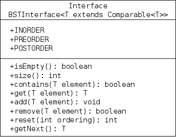
The UML diagram for the interface is shown on the right. It is quite similar to the equivalent diagram for sorted lists.
The main differences between the interfaces for BSTs and for sorted lists occur in the specification of the reset()/getNext() pair. We parameterize reset() so that the pair can traverse the tree in either preorder, inorder, or postorder. Specifically, we define the following three Java constants.
  public static final int INORDER   = 1;
  public static final int PREORDER  = 2;
  public static final int POSTORDER = 3;
In addition, we enhance reset() to return the current size of the tree for so that a user of the pair know how many time to invoke getNext().
Read. The authors re-implement the golf application using binary search trees instead of sorted lists, which illustrates how little changes from the user's viewpoint.
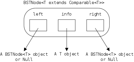
The first order of business is to define the class representing a
node of the tree.
Question: Why can't we
reuse LLNode<T>?
Answer: Those nodes have only one reference to
another node (the successor).
For binary trees we need two such references, on to the left child
and one to the right child.
A detailed picture is on the right.
This node would work fine for any binary tree. That is, it has no dependence on the binary search tree property.
The node would not work for arbitrary trees since it contains references to only two children.
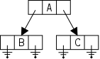
Diagrams of full tree-like structures typically do not show all the Java details in the picture above. Instead, each node would just be three boxes, two containing references to other nodes and the third containing the actual data found in the element. A simplified diagram of a 3-node structure is shown on the right.
Although these simplified diagrams are unquestionably useful, please do not forget the reference semantics that is needed for successfully implementing the concepts in Java.
Question: What would be a good node for an
arbitrary (i.e., non-binary) tree?
Answer: One possibility is to have (in addition
to info) an array of children.
Let's draw it on the board.
Another possibly would be to have two references one to the leftmost
child and the other to the closest
right sibling.
Draw a tree on the board using the normal style and again using the
left-child/right-sibling
style.
  package support;
  public class BSTNode<T extends Comparable<T>> {
    private T info;
    private BSTNode<T> left  = null;
    private BSTNode<T> right = null;

    BSTNode(T info) { this.info = info; }

    public T getInfo()          { return info; }
    public void setInfo(T info) { this.info = info; }

    public BSTNode<T> getLeft()          { return left; }
    public void setLeft(BSTNode<T> link) { left = link; }

    public BSTNode<T> getRight()          { return right; }
    public void setRight(BSTNode<T> link) { right = link; }
  }
The BSTNode<T extends Comparable<T>> implementation is shown on the right. It is straightforward.
To construct a node you supply (a reference to) info and the resulting node has both left and right set to null.
There is a set and a get method for each of the three fields: info, left and right.
(The book chooses to have the constructor explicitly set left and right to null; I prefer to accomplish this via an initialization in the declaration.
A full UML diagram for BSTs is here and at the end of these notes.
  package ch08.trees;
  import ch03.stacks.*;   // used for iterative size()
  import cho4.queues.*    // used for traversals
  import support.BSTNode;

  public class BinarySearchTree<T extends Comparable<T>> {
    private BSTNode<T root = null;
    private found;        // used by remove()
    private LinkUnbndQueue<T> BSTQueue;
    private LinkUnbndQueue<T>  preOrderQueue;
    private LinkUnbndQueue<T> postOrderQueue;

    public boolean isEmpty() { return root == null; }
    public int size() { return recSize(root); }
    // rest later
  } // end of BinarySearchTree<T>
This class will require some effort to implement. The linear nature of stacks, queues, and lists make them easier than trees. In particular removing an element will be seen to be tricky.
The very beginning of the implementation is shown on the right. The only field is root. For an empty tree, which the initial state of a new tree, root is null. Otherwise it references the BSTNode<T> corresponding to the root node.
isEmpty() is trivial, but the rest is not.
The public method size() simply calls the helper recSize(), which is in the next section.
  private int recSize(BSTNode<T> tree) {
    if (tree == null)
      return 0;
    return recSize(tree.getLeft())  +
           recSize(tree.getRight()) +
           1;
  }
The book presents several more complicated approaches before the one shown on the right. The key points to remember are.
Much harder. In some sense you are doing the compiler's job of transforming the recursion to iteration.
In this case, and often with trees, it is no contest: recursion is much more natural and consequentially much easier.
Homework: 20.
Homework: How do you find the maximum element in a binary search tree? The minimum element?
  public boolean contains(T element) {
    recContains(element, root);
  }

  private boolean recContains(T element, BSTNode<T> tree) {
    if (tree == null)
      return false;
    if (element.compareTo(tree.getInfo()) == 0)
      return true;
    if (element.compareTo(tree.getInfo()) < 0)
      return recContains(element, root.getLeft());
    return recContains(element, root.getRight());
  }

  public T get(T element) { return recGet(element, root); }

  public T recGet(T element, BSTNode<T> tree) {
    if (tree == null)
      return null;
    if (element.compareTo(tree.getInfo()) == 0)
      return tree.getInfo();
    if (element.compareTo(tree.getInfo()) < 0)
      return recGet(element, root.getLeft());
    return recGet(element, root.getRight());
  }
The public contains() method simply calls the private helper asking it to search starting at the root.
The helper first checks the current node for the two base cases: If we have exhausted the path down the tree, the element is not present. If we have a match with the current node, we found the element.
If neither base case occurs, we must proceed down to a subtree, the comparison between the current node and the target indicates which child to move to.
get() is quite similar to contains(). The difference is that instead of returning true or false to indicate whether the item is present or not, get() returns (a reference to) the found element or null respectively.
Homework: 31.
The basic idea is straightforward, but the implementation is a little clever. For the moment ignore duplicates, then addition proceeds as follows.
Start searching for the item, this will force you down the tree, heading left or right based on whether the new element is smaller or larger than (the info component of) the current node. Since the element is not in the tree, you will eventually be asked to follow a null pointer. At this point, you create a new node with the given element as info and change the null pointer to reference this new node.
What about duplicates?
Unlike a real search, we do not test if the new element equals (the info component of) each node. Instead, we just check if the new element is smaller. We move left if it is and move right if it isn't. So a duplicate element will be added to the right.
Although add() is short and the basic idea is simple, the implementation is clever and we need to study it on examples. As described above, we descend the tree in the directions determined by the binary search tree property until we reach a null pointer, at which point we insert the element.
  public void add(T element) { root = recAdd(element, root); }

  private BSTNode<T> recAdd(T element, BSTNode<T> tree) {
    if (tree == null) // insert new node here
      tree = new BSTNode<T>(element);
    else if (element.compareTo(tree.getInfo()) < 0)
      tree.setLeft(recAdd(element, tree.getLeft()));
    else
      tree.setRight(recAdd(element, tree.getRight()));
    return tree;
  }
The clever part is the technique used to change the null pointer to refer to the new node. At the deepest recursive level, the setLeft() or setRight() does set a null pointer to a pointer to the new leaf. At other levels it sets a field to the value it already has. This seems silly, but determining when we are making the deepest call (i.e., when the assignment is not redundant) is harder and might cost more than doing the assignment.
Do several examples on the board. Start with an empty tree and keep adding elements.
Then do it again adding the elements in a different order. The shape of the resulting tree depends strongly on the order the elements are added.
Homework: 29, 33.
Start Lecture #21
Remark: Should show that adding the same values in different orders can give very different shaped BSTs.
Whereas the basic idea for add() was clear (the implementation was not); for remove() we first must figure out what to do before we can worry about how to do it.
If the node to be removed is a leaf, then the result is clear: toss the node and change its parent to refer to null.
A minor problem occurs when the leaf to be removed is also the root of the tree (so the tree has only one node). In this case, there is no parent, but we simply make the root data field null, which indicates that the tree is empty. In a rough sense, the root data field acts as the parent of the root node.
The real problem occurs when the node to be removed is not a leaf, especially if it has two children.
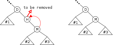
If it has one child, we make the child take the place of its to-be-removed parent. This is illustrated on the right where the node containing H is to be removed. H has one child, M, which, after the removal, has the tree position formerly held by H. To accomplish this removal, we need to change the pointer in H's parent to refer instead to M.
The triangles in the diagram indicate arbitrary (possibly empty) subtrees. When removing a node with one parent all the subtrees remained connected to the same nodes before and after the operation. For some algorithms, however, (in particular for balancing an AVL tree, which we may not study), the subtrees move around.
The dots in the upper right indicate that D may not be the root of the tree. Although the diagram suggests D is a right child, this is not implied. D could be the root, a right child, or a left child.
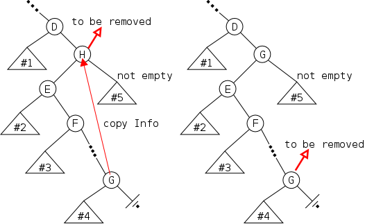
As mentioned this is the hardest case. The goal is to remove node H, which has two children. The diagram shows the procedure used to reduce this case to the ones we solved before, namely removing a node with fewer than 2 children.
The first step is to find H's predecessor, i.e. the node that comes right before H in sorted order. To do this we go left then go as far right as possible arriving at a node G, which definitely has no right child.
The key observation is that if we copy the info from this node to the node we wish to remove, we still have a binary search tree. Since G is before H, any node greater than H is greater than G. Since G is immediately before H, any other node less than H is less than G. Taken together these two fact show that the binary search property still holds.
Now we must remove the original G node. But this node has no right child so the situation is one we already have solved.
  public boolean remove (T element) {
    root = recRemove(element, root);
    return found;
  }
Now that we know what to do, it remains to figure out how to do it. As with node addition, we have a simple public method, shown on the right, that implements the announced specification, and a private helper that does most of the work.
The helper method is assigned two tasks. It sets the data field found, which the public method returns, and the helper itself returns (a reference to) the root of the tree it is given, which the public method assigns to the corresponding data field.
In most cases the root of the original tree doesn't change; however, it can change when the element being removed is located in the root. Moreover, the helper calls itself and when a value is removed the parent's left or right pointer is changed accordingly.
  private BSTNode<T> recRemove(T element, BSTNode<T> tree) {
    if (tree == null) { // element not in tree
      found = false;
      return tree;
    }
    if (element.compareTo(tree.getInfo()) == 0) {
      found = true;  // found the element
      return removeNode(tree);
    }
    if (element.compareTo(tree.getInfo()) < 0)
      tree.setLeft(recRemove(element, tree.getLeft()))
    else
      tree.setRight(recRemove(element, tree.getRight()))
    return tree;
  }
The helper begins with the two base cases. If the tree parameter is null, the element is not present.
If the tree node contains the element we call removeNode() (described below).
In other cases we recursively descend the tree to the left or right depending on the comparison of element and the current node's info. We set the left or right field of the current node to the value of the recursive call. This cleverly assures that the parent of a deleted node has the appropriate field nulled out.
  private BSTNode<T> removeNode (BSTNode<T> tree) {
    if (tree.getLeft() == null)
      return tree.getRight();
    if (tree.getRight() == null)
      return tree.getLeft();
    T data = getPredecessorInfo(tree);
    tree.setInfo(data);
    tree.setLeft(recRemove(data, tree.getLeft()));
    return tree;
  }

  private T getPredcessorInfo(BSTNode<T> tree) {
    tree = getLeft(tree);
    while (tree.getRight() != null)
      tree = tree.getRight();
    return tree.getInfo();
  }
We are given a node to remove and must return (a reference to) the node that should replace it (as the left or right child of the parent or the root of the entire tree).
As usual we start with the base cases, which occur when the node does not have two children. Then we return the non-null child, or null if both children are null.
If the node has two children we proceed as described above. First copy the info from the predecessor to this node and then delete the (actually a) node that contained this data. In this case the reference returned is the unchanged reference to tree.
Subtle, very subtle. It takes study to see when links are actually changed.
Trace through some examples on the board.
Homework: 36,37.
As we have seen in every diagram, trees do not look like lists. However, the user interface we present for trees is quite similar to the one presented for lists. Perhaps the most surprising similarity is the retention of the reset()/getNext() pair for iterating over a tree. Trees don't have a natural next element.
There are two keys to how these dissimilar iterations are made to appear similar, one at the user level and one at the implementation level.
At the user level, we add a parameter orderType
to reset() (the book also adds it
to getNext(), I discuss the pros and cons later).
This parameter specifies the desired traversal order and hence gives
a meaning to the next element
.
Also reset() returns the size of the tree, enabling the user to call getNext() the correct number of times, which is important since getNext() has the additional precondition that it not be called after all items have been returned.
At the implementation level, we have reset() precompute all the next elements. Specifically, we define a queue, let reset() perform a full traversal enqueuing each item visited, and let getNext() simply dequeue one item.
  public int reset(int orderType) {
    BSTQueue = new LinkedUnbndQueue<T>;
    if (orderType == INORDER)
      inOrder(root);
    else if (orderType == PREORDER)
      preOrder(root);
    else if (orderType == POSTORDER)
      postOrder(root);
    return size();
  }

  public T getNext() { return BSTQueue.dequeue(); }
reset() creates a new queue (thus ending any previous iteration) and populates it with all the nodes of the tree.
The order of enqueuing depends on the parameter and is accomplished by a helper method.
The size of the tree, and hence the number of enqueued items, is returned to the user.
getNext() simply returns the next item from the queue.
  private void inOrder(BSTNode<T> tree) {
    if (tree != null) {
      inOrder(tree.getLeft());
      BSTqueue.enqueue(tree.getInfo();
      inOrder(tree.getRight());
    }
  }

  private void preOrder(BSTNode<T> tree) {
    if (tree != null) {
      BSTqueue.enqueue(tree.getInfo();
      preOrder(tree.getLeft());
      preOrder(tree.getRight());
    }
  }

  private void inOrder(BSTNode<T> tree) {
    if (tree != null) {
      postOrder(tree.getLeft());
      postOrder(tree.getRight());
      BSTqueue.enqueue(tree.getInfo();
    }
  }
These three methods, as shown on the right, are direct translations of the pseudocode given earlier. In these particular traversals, visiting a node means enqueuing it on BSTqueue from where they will be dequeued by getNext().
As previously remarked, the three traversals differ only in the placement of the visit (the enqueue) relative to the recursive traversals of the left and right subtrees.
In all three cases the left subtree is traversed prior to the right subtree.
As usual I do things slight differently from the authors. In this subsection, however, I made a real, user-visible change. The book defines three queues, one for each possible traversal. The reset() method enqueues onto the appropriate queue, depending on its parameter. The user-visible change is that getNext() also receives an orderType parameter, which it uses to select the queue to use.
The book's style permits one to have up to three iterations active at once, one using inorder, one preorder, and one postorder. I do not believe this extra flexibility warrants the extra complexity.
A nice test program, that I advise reading. The output from a run is in the book, the program itself is in .../bookFiles/ch08/IDTBinarySearchTree.java
In this comparison, we are assuming the items are ordered. For an unordered collection, a binary search tree (BST) is not even defined.
An array-based list seems the easiest to implement, followed by a linked list, and finally by a BST. What do we get for the extra work?
One difference is in memory usage. The array is most efficient, if you get the size right or only enlarge it by a small amount each time. A linked list is always the right size, but must store a link to the next node with each data item. A BST stores two links.
| BST | Array List | Lnk List | |
|---|---|---|---|
| Constructor | O(1) | O(N) | O(1) |
| isEmpty() | O(1) | O(1) | O(1) |
| reset() | O(N) | O(1) | O(1) |
| getNext() | O(1) | O(1) | O(1) |
| contains()/get() | O(logN) | O(logN) | O(N) |
| add() | O(logN) | O(N) | O(N) |
| remove() | O(logN) | O(N) | O(N) |
The table on the right compares the three implementations we have studied in terms of asymptotic execution time.
The BST looks quite good in this comparison.
In particular, for a large list with high churn
(additions
and removals), it is the clear winner.
The only expensive BST operation is reset() but that is deceptive. If you do a reset, you are likely to perform N getNext() operations, which also costs O(N) in total for all three data structures.
The time for an array-based constructor seems to assume you make the array the needed size initially. Instead of this, we learned how to enlarge arrays when needed.
The book enlarges by a fixed amount, which costs only O(1), but must be applied O(N) to reach a (large) size N. I double the size each time, which costs O(current size), but is only applied O(logN) times. The two methods cost about the same: O(N), which is also the same as needed if we make the array the full size initially.
The good performance attained by a BST depends on it being bushy. If it gets way out of balance (in the extreme example, if it becomes a line) then all the O(logN) boxes become O(N) and the data structure is not competitive.
There are two techniques to keeping the tree balanced, which one
might call the static vs dynamic approaches or might call the manual
vs automatic approaches.
We will take the easy way out
and follow the book by
presenting only the static/manual approach in which the user
explicitly invokes a balance() method when they feel the
tree might be imbalanced.
We will not consider the automatic approach in which the add and
remove operations themselves ensure that the tree is always
balanced.
Anyone interested in the automatic should type AVL tree
into
Google.
We will consider only the following 2-step approach.
For step 1 we presumably want to traverse the BST, but which traversal.
For step 2 we presumably want to use the BST add() method, but what order should we choose the elements from the array?
If we employ inorder and place consecutive elements into
consecutive array slots, the array is sorted.
If we then use add() on consecutive elements
(the natural
order), we get a line.
This is the worst possible outcome!
Now extract the elements with preorder and again add them back using consecutive elements of the array. This procedure is the identity, i.e., we get back the same tree we started with. A waste of time.
This procedure is harder to characterize, but it does not produce balanced trees. Let's try some.
Middle First
  balance()
    n = tree.reset(INORDER);
    for (int i=0; i<n; i++)
      array[i] = tree.getNext()
    tree = new BinarySearchTree()
    tree.insertTree(0, n-1)
The code on the right shows the choice of inorder traversal.
Recall that reset() returns the current size of the tree,
which tells us how many times to execute getNext().
The fifth line on the right produces a new (empty) tree.
We now need to specify insertTree(), i.e., explain the cryptic
Middle First
.
Since we use Inorder, the array is sorted. Whatever element we choose to add first will become the new root. For the result to be balanced, this element should be the middle of the sorted list. With a sorted array, the middle element is easy to find.
  insertTree(lo, hi)
    if (hi == lo)
      tree.add(array[lo])
    if (hi == lo+1)
      tree.add(array[lo]
      tree.add(array[hi]
    mid = (lo+hi)/2
    tree.insertTree(lo, mid-1)
    tree.insertTree(mid+1, hi)
Now that the root is good, what is next. If we pick an element smaller than the middle it will become (and remain) the left child of the root. We want this tree node to have as many left as right descendants so we want the middle of the numbers smaller than our original middle. Etcetera.
This analysis gives rise to the algorithm on the right. If we have one or two elements we insert both (in either order; these are the base cases). Otherwise, insert the middle element and then insert the remaining small ones followed by inserting the remaining large ones (or vice-versa).
Homework: 46.
Start Lecture #22
Remark: Lab 5, the last lab, is posted.
The basic idea is easy. Use the following algorithm to store the binary tree in an array.
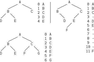
On the right we see three examples. The upper left example has 5 nodes. The root node A is stored in slot 0 of the array; it's left and right children are stored in slots 2*0+1 and 2*0+2 respectively.
The lower left is similar, but with 7 nodes.
The right example only has 6 nodes but requires 12 array slots, because some of the planed-for children are not in the tree, but array slots have been allocated for them.
Let's check that the rules for storing left and right children are satisfied for all three examples.
Definition: A binary tree like the one on the lower left in which all levels are full is called full.
Definition: A binary tree like the one on the upper left in which the only missing nodes are the rightmost ones on the last level is called complete.
The following properties are clear.
The array tree has the advantage that the parent (of a non-root node) can be found quickly. Its disadvantages are that, if the tree is not complete, space is wasted and, if an addition requires the array to have more slots than originally allocated, we must enlarge the array (or raise an exception).
Homework: 48,49.
Read.
A BST is an effective structure for storing sorted items. It does require two links per item, but essentially all operations are fast O(logN), providing the tree remains balanced. We presented an algorithm for explicitly re-balancing a BST and reference AVL trees as an example of BSTs that are automatically balanced.
First things first. A priority queue is not a queue. That is, it does not have FIFO semantics. I consider it a bad name, but it is much too late to try to change the name as it is absolutely standard.
In a priority queue, each item has an associated priority and
the dequeue
operation (I would call it remove since it is not
removing the first-in item) removes the enqueued
item with the
highest priority.
The priority of an item is defined by the Java class of the items.
In particular, we will normally assume x has higher
priority than y if x.compareTo(y)>0.
In fact sometimes the reverse is true and smaller
items
(according to compareTo() have higher priority.
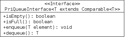
We see the uml diagram on the right. It is quite simple: tests for full and empty and mutators that insert and remove an element.
The inclusion of isFull() suggests that we are using a bounded structure to hold the elements and indeed some implementations will do so. However, we can use an unbounded structure and just have isFull() always return false.
We specify that enqueuing onto a full queue or dequeuing from an empty queue raises an (unchecked) exception
In 202, when you learn process scheduling, you will see that often
an operating system wishes to run the highest priority
eligible process.
We can also think of the triage system used at hospital emergency rooms as another implementation of priority scheduling and priority queues.
A real, (i.e., FIFO) queue is also a priority queue. The priority is then the negative of the time at which the enqueue occurs. With this priority the earliest enqueued item has the highest priority and hence is dequeued first.
The general point is that when the next item not picked at random, often some sort of (often not explicitly stated) priority is assigned to the items and the one selected scores best using this metric.
We are not short of methods to implement a priority queue. Indeed, we have already implemented the following four such schemes. However, each has a defect when used for this application.
Enqueuing is trivial, just append, and fast O(1). Dequeuing, however, requires that we scan the entire list, which is slow O(N), where N is the number of items.
We now have the reverse situation: Dequeuing is O(1) since the highest priority item is the last item, but enqueuing is O(N) since we have to shift elements down to make room for the new one (finding the insertion site is O(logN) if we use binary search and thus is not rate limiting).
Dequeuing is O(1) providing we sort the list in decreasing order. But again enqueuing is O(N).
Probably the best of the bunch. For a balanced BST, both enqueuing and dequeuing are O(logN), which is quite good. For random insertions the tree will likely be balanced but in the worst case (e.g., if the insertions come in sorted order) the tree becomes a line and the operations take O(N).
We can balance the tree on occasions, but this operation is always O(N).
The biggest problem with AVL trees is that we don't know what they are. They are also the fifth of the "four such schemes". Had we studied them or some other auto-balanced BST we would have seen that all operations are O(logN).
The AVL algorithms are somewhat complicated and AVL trees are overkill. We don't need to find an arbitrary element, just the largest one. Could we perhaps find a simpler O(logN) set of algorithm solving our simpler problem?
Yes we can and we study one next.
Homework: 3,4.
In future courses you will likely learn about regions of memory call the stack and the heap.
The stack region is used to store variables that have stack-like lifetimes, i.e. the first ones created are the last ones destroyed (think of f calls g and g calls h).
So the stack region is related to the stacks we have studied. However, the heap region is not related to the heaps we will study now.
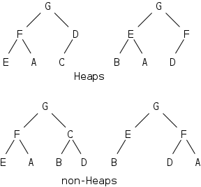
Definition: A heap is a complete binary tree in which no child has a greater value than its parent.
Note that this definition includes both a shape property and an order property.
On the right we see four trees where each node contains a Character as its info field.
Question: Why are the bottom two trees not
heaps?
The left tree violates the order property since the right child of C
is greater than C.
The right tree is not complete and thus violates the shape
property.
Homework: 6, 7 (your example should have at least 4 nodes).
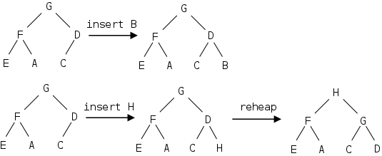
The picture on the right shows the steps in inserting a new element B into the first heap of the previous diagram.
Since the result must be a complete tree, we know where the new element must go. In the first row, all goes well the result of placing B in the required position yields another heap.
In the second row, we want to insert H instead of B and the result is not a heap since the order property is not satisfied. We must shift some elements around. The specific shifting that we will do, results in the rightmost tree.
An sequence of insertions is shown below, where, for variety, we use a heap in which smaller elements have higher priority. In each case the reheaping, often called a sift-up, consists of a sequence of local operations in which the inserted item is repeatedly compared with its parent and swapped if the ordering is wrong.
Let's make sure we understand every one of the examples.
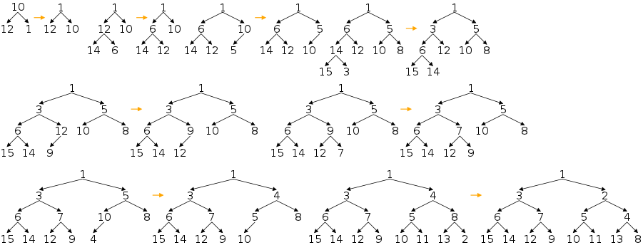
We know that the highest priority element is the root so that is the element we must delete, but we also know that to maintain the shape property the position to be vacated must be the rightmost on the bottom row.
We meet both requirements by temporarily deleting the root, which we return to the user, and then moving the rightmost bottom element into the root position. But the result is probably not a heap since we have a just placed a low priority item into the slot reserved for the highest priority item.
We repair this damage by performing sift-downs, in which the root element is repeatedly swapped with its higher priority (in this example that means smaller) child.
On the board, start with the last tree from the previous diagram and perform several deletions. Note that the result of each delete is again a heap and hence the elements are removed in sorted (i.e., priority) order.
A key point in the heap implementation is that we use the array representation of a binary tree discussed last chapter. Recall that the one bad point of that representation was that when the tree is sparse, there may be many wasted array slots. However, for a heap this never the case since heaps are complete binary trees.
As I have mentioned Java generics have weaknesses, perhaps the most important of which is the inability to create generic arrays. For this reason the book (perhaps wisely) uses the ArrayList class from the Java library instead of using arrays themselves.
However, we have not yet used ArrayList in the regular section of the course and it does make the code look a little unnatural to have elements.add(i,x); rather than the familiar elements[i]=x;
For this reason I rewrote the code to use the normal array syntax
and that is what you will see below.
But, this natural code does not run and must
be doctored
in order to execute successfully.
In particular, various casts are needed and I offer a link to a
working (albeit ugly)
version here.
You should view the version in the notes as a model of what is
needed and the referenced working version as one way to bend it to
meet Java's weakness with generic arrays.
  package priorityQueues;
  class PriQOverflowException extends RuntimeException {
    public PriQOverflowException() { super(); }
    public PriQOverflowException(String message) {
      super(message);
    }
  }

  package priorityQueues;
  class PriQUnderflowException extends RuntimeException {
    public PriQUnderflowException() { super(); }
    public PriQUnderflowException(String message) {
      super(message);
    }
  }
Since we are basing our implementation on fixed size arrays, overflows occur when enqueuing onto a full heap. Underflows always occur when dequeuing any empty structure.
We follow the book and have underflows and overflows each trigger a java RuntimeException. Recall that these are unchecked exceptions so a user of the package does not need to catch them or declare that it might throw them.
Each of our exceptions simply calls the constructor in the parent class (namely RuntimeException.
package priorityQueues;
public class Heap<T extends Comparable<T>>
       implements PriQueueInterface<T> {
  private T[] elements;
  private int lastIndex = -1;
  private int maxIndex;

  public Heap(int maxSize) {
    elements = new T[maxSize];
    maxIndex = maxSize - 1;
  }
As with BSTs, heaps have an inherent order among their elements. Hence we must again require that T extends Comparable<T>.
Recall that the heap will be implemented as an array. maxIndex is essentially the physical size of the array; whereas, lastIndex, designating the highest numbered full slot is essentially the size of the heap since all lower slots are also full.
The constructor is given the size of the array from which it
creates the array and the largest possible index.
We know that the new statement is illegal.
In previous array-based structures
(e.g., ArrayUnsortedList), a simple
cast fixed
the problem, but here more work was needed (see my
doctored code.
  public boolean isEmpty() { return lastIndex == -1; }
  public boolean isFull()  { return lastIndex == maxIndex; }
These are trivial.
  public void enqueue (T element)
         throws PriQOverflowException {
    if (lastIndex == maxIndex)
      throw new PriQOverflowException("helpful message");
    lastIndex++;
    reheapUp(element);
  }

  private void reheapUp(T element) {
    int hole = lastIndex;
    while ((hole>0) &&
           (element.compareTo(elements[parent(hole)])>0)) {
      elements[hole] = elements[parent(hole)];
      hole = parent(hole);
    }
    elements[hole] = element;
  }

  private int parent(int index) { return (index-1)/2; }
If the heap is filled, enqueue() raises an exception; otherwise it increases the size of the of the heap by 1.
Rather than placing the new item in the new last slot and then
swapping it up to its final position, we place a hole
in the
slot and swap the hole up instead.
We place the new item in the hole's final location.
This procedure is more efficient since it takes only two assignments to swap a hole and an element, but takes three to swap two elements.
To make the code easier to read I recompute the parent's index twice and isolate the computation in a new method. It would be more efficient to compute it once inline; an improvement that an aggressive optimizing compiler would perform automatically.
  public T dequeue() throws PriQUnderflowException{
    if (lastIndex == -1)
      throw new PriQUnderflowException("Helpful msg");
    T ans    = elements[0];
    T toMove = elements[lastIndex--];
    if (lastIndex != -1)
      reheapDown(toMove);
    return ans;
  }

  private void reheapDown(T element) {
    int hole = 0;
    int newhole = newHole(hole, element);
    while (newhole != hole) {
      elements[hole] = elements[newhole];
      hole = newhole;
      newhole = newHole(hole, element);
    }
    elements[hole] = element;
  }

  private int newHole(int hole, T element) {
    int left  = 2 * hole + 1;
    int right = 2 * hole + 2;
    if (left > lastIndex)    // no children
      return hole;
    if (left == lastIndex)   // one child
      return element.compareTo(elements[left])<0? left: hole;
    if (elements[left].compareTo(elements[right]) <  0)
      return element.compareTo(elements[right])<0? right: hole;
    return element.compareTo(elements[left])<0? left: hole;
  }
If the queue is empty, dequeue() raises and exception; otherwise it returns the current root to the user and hence decreases the heap's size by 1. Removing the root leaves a hole there, which is then filled with the current last item, restoring the shape property.
But elevating
the last item is likely to violate the order
property.
This violation can be repaired by successively swapping the item with
its larger child.
Instead of successively swapping two items, it is again more efficient to successively swap the hole (currently the root position) with its larger child and only at the end move the last item into the final hole location.
The process of swapping the hole down the tree is called sift-down or reheap-down.
Finding the larger child and determining if it is larger than the parent is easy but does take several lines so is isolated in the newhole() routine.
  // for testing only
  public String toString() {
    String theHeap = new String("The heap is\n");
    for (int i=0; i<=lastIndex; i++)
      theHeap += i + ".  " + elements[i] + "\n";
    return theHeap;
  }
}
A useful aid in testing the heap and many other classes, is to override the toString() method defined for any Object.
Since a heap is implemented as an array, the code on the right, which just lists all the array slots with their corresponding indices, is quite useful for simple debugging.
A heap would user would likely prefer a graphical output of the corresponding tree structure, but this is more challenging to produce.
Start Lecture #23
Remark: As guessed the (hole>1) was a typo and has been fixed. Note that the book's test case worked fine on both the wrong and corrected version. The limitation of (not extensive) testing.
| enqueue | dequeue | |
|---|---|---|
| Linked List | O(N) | O(1) |
| Heap | O(logN) | O(logN) |
| Binary Search Tree | ||
| Balanced | O(logN) | O(logN) |
| Skewed | O(N) | O(N) |
The table on the right compares the performance of the various structures used to implement a priority queue. The two winners are heaps and balanced binary search trees.
Our binary search trees can go out of balance and we need to judiciously choose when to re-balance (an expensive O(N) operation).
As mentioned there are binary search trees (e.g. AVL trees) that maintain their balance and still have the favorable O(logN) performance for all operations. However, these trees are rather complicated and are overkill for priority queues where we need only find the highest element.
Homework: 10, 11.
We discussed priority queues, which can be implemented by several data structures. The two with competitive performance are the binary search tree and the heap. The former is overkill and our BST implementations did not fully address the issue of maintaining balance.
In this chapter we described a heap in detail including its implementation. Since heaps are complete binary trees an array-based implementation is quite efficient.
We skipped the material on graphs.
Given an unsorted list of elements, searching is inherently slow (O(N)) whether we seek a specific element, the largest element, the smallest element, or the element of highest/lowest priority.
In contrast a sorted list can be searched quickly:
But what if you are given an unsorted list and want it sorted? That is the subject of this chapter together with other searching techniques that in many cases can find an arbitrary element in constant time.
Sorting is quite important and considerable effort has been given to obtaining efficient implementations.
It has been proven that no comparison-based
sorting algorithm can do better than O(NlogN).
We will see algorithms that achieve this lower bound as well as
simpler algorithms that are slower (O(N2)).
Roughly speaking a sorting algorithm is comparison-based if it sorts by comparing elements of the array. Any natural algorithm you are likely to think of is comparison-based. In basic algorithms you will see a more formal definition.
We will normally write in-place
sorting algorithms that do
not use significant space outside the array to be sorted.
The exception is merge sort.
public class TestSortingMethod {
  private static final int SIZE = 50;
  private static final int DIGITS = 3;  // change printf %4d
  private static final int MAX_VALUE = (int)Math.pow(10,DIGITS)-1;
  private static final int NUM_PER_LINE = 10;
  private static int[] values = new int[SIZE];
  private static int numSwaps = 0;

  private static void initValues() {
    for (int i=0; i<SIZE; i++)
      values[i] = (int)((MAX_VALUE+1)*Math.random());
  }

  private static boolean isSorted() {
    for (int i=0; i<SIZE-1; i++)
      if (values[i] > values[i+1])
    return false;
    return true;
  }

  private static void swap (int i, int j) {
    int t = values[i];
    values[i] = values[j];
    values[j] = t;
    numSwaps++;
  }

  private static void printValues() {
    System.out.println("The value array is:");
    for (int i=0; i<SIZE; i++)
      if ((i+1) % NUM_PER_LINE == 0)
    System.out.printf("%4d\n", values[i]);
      else
    System.out.printf("%4d"  , values[i]);
    System.out.println();
  }

  public static void main(String[] args) {
    initValues();
    printValues();
    System.out.printf("The array %s initially sorted.",
              isSorted() ? "is" : "is not");
    sortValues();
    printValues();
    System.out.printf("After performing %d swaps,\n", numSwaps);
    System.out.printf("the array is %s sorted.",
                      isSorted() ? "now" : "still not");
  }

  private static void sortValues() {
    // call sort program here
  }
}
Since we will have several sort routines to test we write a general
testing harness
into which we can plug any sorting routing
that sorts an int[] array named values.
The harness initializes values to random non-negative integers, prints the values, checks if the initial values are sorted (probably not), calls the sort routine in question, prints the array again, and checks if the values are now sorted.
In order to be flexible in testing, the harness uses three configuration constant, SIZE, the number of items to be sorted DIGITS the number of digits in each number, and NUM_PER_LINE, the number of values printed on each line.
The maximum value (used in generating a problem) is calculated from DIGITS, but the %4d in printf() must be changed manually.
The following output is produced when the configuration constants are set as shown on the right.
The values array is:
 513 190 527 324 930 948 504 228  37 891
 153 277 552 893 738 926 193 408 525 324
 178 389 738 784 728 812 783 558 530 703
 843  38  53 999 326  34 777 496 915 364
 929 576 937 572  43 439 569 245 740  53

The array is not initialy sorted.

The values array is:
 513 190 527 324 930 948 504 228  37 891
 153 277 552 893 738 926 193 408 525 324
 178 389 738 784 728 812 783 558 530 703
 843  38  53 999 326  34 777 496 915 364
 929 576 937 572  43 439 569 245 740  53

After performing 0 swaps,
the array is still not sorted.
For convenience, a swap() method is provided that keeps track of how many swaps have been performed.
These algorithms are simple (a virtue), but slow (a defect). They are the obvious choice when sorting small arrays, say a hundred or so entries, but are never used for serious sorting problems with millions of entries.
I am not sure what the adjective straight
means here.
The idea behind selection sort is simple.
  private static void selectionSort() {
    for (int i=0; i<SIZE-1; i++)
      swap(i, minIndex(i, SIZE-1));
  }
  private static int minIndex(int startIndex, int endIndex) {
    int ans = startIndex;
    for (int i=startIndex+1; i<=endIndex; i++)
      if (values[i] < values[ans])
    ans = i;
    return ans;
  }
The code, shown on the right is also simple.
The outer loop (selectionSort() itself) does
the etcetera
.
That is, it causes us to successively swap the first with the
minimum, the second with the minimum from 2 down, etc.
The minIndex routine finds the index in the given range whose slot contains the smallest element. For selectionSort(),endIndex could be omitted since it is always SIZE-1, but in other sorts it is not.
Selection sort is clearly simple and we can see from the code that it uses very little memory beyond the input array. However, it is slow.
The outer loop has N-1 iterations (N is SIZE, the size of the problem). The inner loop first has N-1 iteration, then N-2, ..., finally 0 iterations.
Thus the total number of comparisons between two values is
N-1 + N-2 + N-3 + ... + 1
You will learn in basic algorithms that this sum equals
(N-1)(N-1+1)/2=O(N2), which is horrible when say
N=1,000,000.
  private static void bubbleSort() {
    boolean sorted = false;
    while (!sorted) {
      sorted = true;
      for (int i=0; i<SIZE-1; i++)
        if (values[i] > values[i+1]) {
          swap(i, i+1);
          sorted=false;
        }
    }
  }
Bubble and selection sorts both try to get one element correct and then proceed to get the next element correct. (For bubble it is the last (largest) element that is corrected first.) A more significant difference is that bubble sort only compares and swaps adjacent elements and performs more swaps (but not more comparisons).
There are several small variations on bubble sort.
The version on the right is one of the simplest.
Although there are faster versions they are
all O(N2) in the worst case so are never used
for large problems unless the problems are known to be almost
sorted
.
This analysis is harder than for selection sort; we shall skip it.
  private static void insertionSort() {
    for (int i=1; i<SIZE; i++) {
      int j = i;
      while (j>0 && values[j-1]>values[j]) {
        swap(j, j-1);
        j--;
      }
    }
  }
For this sort we take each element and insert it where it belongs in the elements sorted so far. Initially, the first element is itself sorted. Then we place the second element where it belongs with respect to the first, and then the third with respect to the first two, etc.
In more detail, when elements 0..i-1 have been sorted, swap element i with elements i-1, i-2, ..., until the element is in the correct location.
The best case occurs when the array is already sorted, in which case the element comparison fails immediately and no swaps are done.
The worst case occurs when the array is originally in reverse order, in which case the compares and swaps always go all the way to the first element of the array. This again gives a (worst case) complexity of O(N2)
Homework: 2,5,6,8.
These are the ones that are used for serious sorting.
  private static void mergeSort(int first, int last) {
    if (first < last) {
      int middle = (first+last) / 2;
      mergeSort(first, middle);
      mergeSort(middle+1, last);
      merge(first, middle, last);
    }
  }
  private static void merge(int leftFirst, int leftLast, int rightLast) {
    int leftIndex = leftFirst;
    int rightIndex = leftLast+1;
    int[] tempArray = new int[rightLast-leftFirst+1];
    int tempIndex = 0;
    while (leftIndex<=leftLast  &&  rightIndex<=rightLast)
      if (values[leftIndex] < values[rightIndex])
	tempArray[tempIndex++] = values[leftIndex++];
      else
	tempArray[tempIndex++] = values[rightIndex++];
    while (leftIndex <= leftLast)
      tempArray[tempIndex++] = values[leftIndex++];
    while (rightIndex <= rightLast)
      tempArray[tempIndex++] = values[rightIndex++];
    for (tempIndex=0; tempIndex<tempArray.length; tempIndex++)
      values[leftFirst+tempIndex] = tempArray[tempIndex];
  }
The mergesort routine itself might look too simple to work, much less to be one of the best sorts around. The reason for this appearance is its recursive nature. To mergesort the array, use mergesort to sort the first half, then use mergesort to sort the second half, then merge these two sorted halves.
Merging two sorted lists is easy. I like to think of two sorted decks of cards.
Compare the top card of each pile and take the smaller. When one of the piles is depleted, simply take the remainder of the other pile.
Note that the tempArray for the last merge performed is equal in size to the initial array. So merge sort requires O(N) additional space, a disadvantage.
The analysis is harder than the program and I leave the details for basic algorithms. What follows is the basic idea.
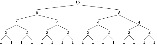
To simplify slightly let's assume we are sorting a power of two
numbers.
On the right is the merge tree
for sorting 16=24
values.
From the diagram we see 31 calls to mergeSort(), one of size 16, two of size 8, ..., 16 of size 1. For any power of two there will be 2N-1calls if we are sorting N, a power of 2, values.
MergeSort() itself is trivial, just 3 method calls, i.e. O(1), and hence all the calls to mergeSort() combined take O(N).
What about the calls to merge()? Each /\ in the diagram corresponds to a merge. If you look at the code for Merge(), you can see that each call is O(k), when you are merging k values. The bottom row of the diagram contains 8 merges, each merging two values. The next row contains 4 merges, each of 4 values. Indeed, in each row N=16 elements are merged it total. So each row of merges requires O(N) effort.
Question: How many rows are there?
Answer: logN.
Hence the total effort for all the merges is O(NlogN). Since all the mergeSort() routines take only O(N), the total effort for mergesort is O(NlogN) as desired.
Homework: 11,12.
This algorithm is obvious
but getting it right is hard as
there are many details and potential off by one
pitfalls.
Like mergeSort(), quickSort() recursively divides the array into two pieces which are sorted separately. However, in this algorithm one piece has all the small values, the other all the large ones. Thus there is no merging needed.
The recursion ends with a base case in which the piece has zero of one items and thus is already sorted.
| all ≤ X | X | all >X |
The idea is that we choose one of the values in the array (call it X) and swap elements so that everything in the left (beginning) part of the array is less than or equal to X, everything in the right part is greater than X, and X is in between the two parts.
Now X is correctly located and all we need to do is sort each of the two parts. The clever coding is needed to do the swapping correctly.
We will do examples on the board, but not study the coding. All the sorting algorithms are available here.
The speed depends on how well the array is divided. If each piece is about 1/2 size, the time is great O(NlogN). If one piece is extremely small, the time is poor O(N2).
The key to determining the sizes of the pieces is the choice X above. In my code, X is set to the first value in the interval to be reordered. Like any other choice of X, this can sometimes be bad and sometimes be good.
It should be noted that, if the original array is almost sorted, this choice of X is bad. Since such arrays often arise in practice, real quicksort programs use a different X. The book suggests the middle index in the range; others suggest taking the first, last, and middle index and choosing the one whose value is in the middle of the three.
Any of these choices have as many bad cases as any other, the point of using something other than simply the first entry is that for the others the bad cases are not as common in practice as an almost sorted array.
  private static void heapSort() {
    PriQueueInterface<Integer> h = new Heap(values.length);
    for (int i=0; i<values.length; i++)
      h.enqueue(values[i]);
    for (int i=values.length-1; i>=0; i--)
      values[i] = h.dequeue();
  }
On the right is a simple heapsort using our heap from chapter 9. I am surprised the book didn't mention it.
A disadvantage of the simple heapsort is that it uses an extra array (the heap h). The better algorithm in the book builds the heap in place so uses very little extra space.
Although the values array is not a heap, it does satisfy the shape property. Also, all the leaves (the array entries with the largest indices) are valid subheaps so we start with highest-indexed, non-leaf and sift it down using a variant ofreheapDown() from chapter 9. Then we proceed up the tree and repeat the procedure.
I added an extra print to heapsort in the online code to show the array after it has been made into a heap, but before it has become sorted.
Now that we have a heap, the largest element is in values[0]. If we swap it with values[SIZE-1], we have the last element correct and hence no longer access it.. The first SIZE-1 elements are almost a heap, just values[0] is wrong. Thus a single reheapDown() restores the heap and we can continue.
Homework: 19, 22, 23
All the sorting algorithms are implemented here embedded in the test harness developed earlier. To run the a given sorting program, go to the sortValues() method and comment out calling all the other sorts.
Several good general comments about testing as applied to sorting.
  public static void badSort(int[] a) {
    for (i=0; i<a.length; i++)
      a[i] = i;
  }
However, there is an important consideration that is not normally
discussed and that is rather hard to check.
Executing the method on the right results
in a being sorted
; however, the
result bears little resemblance to the original array.
Many sort checkers would
validate badSort().
We have paid little attention to small values of N. The real concern is not for small problems; they are fast enough with any method. The issue arises with recursive sorts. Using heapsort, mergesort, or quicksort on a large (say 1,000,000) entry array results in very many recursive calls to small subproblems that can be solved more quickly with a simpler sort.
Good implementations of these recursive algorithms call a simpler sort when the size of the subproblem is below a threshold.
Method calls are not free. The overhead of the call is especially noticeable when a method with a small body called often. Programmers and good compilers can eliminate many of these calls.l
Most of the time minor performance improvements such as eliminating method calls are not made ... with good reason. The primary quality metric for all programs is correctness. For most programs, performance is not the second quality metric; instead ease of modification, on time completion, and cost rank higher. Cost is basically programmer time so it is not wise to invest considerable effort for small performance gains.
Note that the preceding paragraph does not apply to the huge gains that occur in large problems when a O(NlogN) algorithm replaces an O(N2) algorithm.
The only significant difference in storage space required is between those algorithms (mergesort and quicksort) that require extra space proportional to the size of the array and those that do not. Normally, we worry more about time than space, but the latter does count.
You might worry that if we are sorting large objects rather than primitive int's or tiny Character's, that swapping elements. For example, if we had an array of String's and it turned out that each string was a book containing about a million characters, then swapping two of these String's would be very expensive indeed.
But that is wrong!
The swaps do not actually swap the million character strings but swap the (small) references to the strings.
We have used this interface many times. The only new point in this section is to note that a class can have only one CompareTo() method and thus can only be sorted on one basis.
There are cases where you want two different orderings. For example, you could sort airline flights on 1 March from NYC to LA by time of day or by cost for the cheapest coach ticket. Comparable does not offer this possibility.
The somewhat more complicated Comparitor interface is based on a compare() method with two parameters, the values to be compared. The interesting part is the ability to have multiple such methods. However, we will not pursue this interface further.
A sort is called stable if it preserves the relative order of duplicate values. This becomes important when an object has several fields and you are only sorting based on one field. Thus duplicated objects need only have the sorted field equal and hence duplicates are not necessarily identical.
Assume you first sort on one field and then on a second. With a stable sort you are assured that items with equal second field have their first fields in order.
Sometimes searching is not needed. If we have an indexed list implemented with an array A of objects of some class C, then obtaining entry number 12 is simply retrieving A[12], a constant time (i.e., O(1) operation.
To be specific, assume C consists of NYU students and an object in C contains the students name, N number, and major. Then finding the major of the student in entry 12 is simply A[12].NNumber, again an O(1) operation.
However, many times the easy solution above is not possible.
For example, with the same implementation finding the entry number
of a student named Tom Li
require searching, as does
finding Li's major.
Linear searching (trying the first object, then the second, etc.) is always possible, but is slow (O(N) for N objects).
In many circumstances, you know that there will be popular
and unpopular
object.
That is, you know there will be some objects searched for much
more frequently than others.
If you know the identity of the popular objects you can place them
first so that linear search will find them quickly.
But what if you know only that there are popular objects but don't
know what they are?
In this last situation the move to the front
algorithm
performs well (I often use it for physical objects).
When you search for and find an object, move it to the front of
the list (sliding objects that preceded it down one slot).
After a while this will have popular objects toward the front and
unpopular objects toward the rear.
For physical objects (say documents) it is often O(1) to move a found object to the front. However, for an array the sliding down can be O(N). For this reason, an approximation is sometimes used where you simply swap the found object with the first, clearly an O(1) task.
Knowing that a list is sorted helps linear search and often permits the vastly faster binary search.
When linearly searching a sorted list for an element that is not present, one can stop as soon as the search passes the point where the item would have been stored, reducing the number of items search to about half on average.
More significantly, for an array-based sorted list we can use the O(logN) binary search, a big speed advantage.
Start Lecture #24
We learned that if a list is unsorted we can find an element in the list (or determine that the element is not there) in time O(N) using linear searching (try the first, then the second, etc.).
If the list is sorted we can reduce the searching time to O(logN) by using binary search (roughly: try the middle, then the middle of the correct half, then the middle of the correct quarter, etc.).
Can we ever hope to find an element in a list using a constant amount of time (i.e., the time to lookup an element does not depend on the number of elements?
In fact this is sometimes possible. I found on the web the roster of this year's NY Jets football team. Assume you have an array of strings NYJets with NYJets[11]="Kerley", NYJets[21]="Bell", NYJets[18]="*", etc. Then you can answer questions like these in constant time.
We say that the player number is the key.
But this case is too easy. Not only are there very few entries, but the range of indices is small.
Now consider a similar list of the students in this class with key
their their NYU N numbers
.
Again there are very few entries (about 50), but now the range of
indices is huge.
My N number has 8 digits so we would need an array of 100,000,000
entries with all but 50 being "*".
This situation is when hashing is useful.
The book makes the following three assumptions to simplify the discussion.
Some comments on these assumptions.
Instead of indexing the array by our N numbers, instead take just the last 3 digits (i.e., compute (N number) % 1000). Now we only need an array of size 1,000 instead of 100,000,000.
Definition: The function mapping the original key to another (presumably smaller) value, which is then used to access the table, is called a hash function.
For now we will use the above hash function, i.e., we take the key modulo the size of the table.
All is well, searching is O(1), PROVIDING no two N numbers in the class end in the same three digits, i.e., providing we have no collisions.
  public class Student {
    private int nNumber;	// the key
    private String name;
    private String major;
    // etc
    public Student(int nNumber, String name, String major) {
      this.nNumber = nNumber;
      this.name    = name;
      this.major   = major;
    }
    public int    getNNumber() { return nNumber; }
    public String getName()    { return name;    }
    public String getMajor()   { return major;   }

    public void   setNNumber(int nNumber) { this.nNumber = nNumber; }
    public void   setname(String name)    { this.name    = name;    }
    public void   setMajor(String major)  { this.major   = major;   }
  }

  public class StudentHashtable {
    private Student[] studentHashtable;
    private int size;
    public StudentHashtable(int size) {
      this.size = size;
      studentHashtable = new Student[size];
    }

    public int hash(int key) { return key % size; }

    public void add (Student s) {
      studentHashtable[hash(s.getNNumber())] = s;

    public Student get(Student s) {
      return studentHashtable[hash(s.getNNumber())];
    }
  }
Although we will not be developing hashtables to the point of actual code, I thought it would be helpful to see a possible basic setup.
It would be better to have a generic hashtable class that accepted as type parameter (the <T> business) the type of object being stored, I didn't want to battle with generic arrays since we aren't actually going to use the implementation.
So I was inelegant and made the class specific to the object being stored, in this case Student.
I defined a standard hash() method taking and returning an int. Were we developing a complete implementation, I might have defined it as taking a Student as input and then have hash() itself extract the nNumber, which it would then use as key.
Our add() is easy.
The get() method returns the entry from the hashtable that is equal to the argument.
Something must be wrong. This is too easy.
A minor simplification is that we assume there is room for the element we add and are assuming the element we are asked to get is present. We could fix the former by keep track of the size; and fix the latter by checking the found entry and returning null if it doesn't match.
The real simplification is that we assume collisions don't happen. That is we assume that different keys are hashed to different values. But this is clearly not guaranteed. Imagine we made a 1000 entry table for NYU students and picked say 900 students. Our hash function just returns the last three digits of their N number. I very much doubt that 900 random NYU students all have unique 3-digit N number suffixes. Collisions do and will happen. The question is what to do when they occur, which is our next topic.
One can attack collisions in two ways: minimize their occurrence and reduce the difficulty they cause. We will not do the former and will continue to just use the simple mod function.
One place where collisions occur is in the add() method. Naturally, if you add an element twice, both will hash to the same place. Let's ignore that possibility and say we never add an element already present. When we try to add an element, we store the element in the array slot given by the hash of the key. A collision occurs when the slot already contains a (different) entry.
We need to find a location to store an item that hashes to the same value as an already stored item. There are two classes of solutions: open addressing and separate chaining.
  public void add (Student s) {
    int location = hash(s.getNNumber());
    while (studentHashtable[location] != null)
      location = (location+1) % capacity;
    studentHashtable[location] = s;
  }

  public Student get(Student s) {
    int location = hash(s.getNNumber());
    while (studentHashtable[location].getNNumber()!=s.getNNumber())
      location = (location+1) % capacity;
    return studentHashtable[location];
  }
The simplest example of open addressing is linear probing. When we hash to a full slot, we simply try the next slot, i.e., we increase the slot number by 1 (mod capacity).
The new versions of add() and get() are on the right. The top loop would not terminate if the table is full; the bottom loop would not terminate if the item was not present. However, we are assuming that neither of these conditions holds.
As mentioned above it is not hard to eliminate these assumptions.
Homework: 42
More serious is trying to support delete and search.
| 13 | 23 |
Let the capacity be 10 and do the following operations.
Insert 13; Insert 24;
Insert 23; Delete 24;
The result is shown on the right.
If you now look for 23, you will first try slot 3 (filled with 13) and then try slot 4 (empty since 24 was deleted). Since 23 would have gone here, you conclude erroneously that it is not present.
| 13 | ** | 23 |
The solution is not to mark a deleted slot as empty (null) but instead as deleted (I will use **). Then the result looks as shown on the right and an attempt to find 23 will proceed as follows. Try slot 3 (filled with 13), try 4 (a deleted item), try slot 5 (success).
A problem with open addressing, particularly with linear probing
is that clusters develop.
After one collision we now have a block of two elements that hash to
one address.
Hence the next addition will be in this cluster
if it hashes
to either of the two address.
With a cluster of three, now any new item that hashes to one of the
three will add to the cluster.
In general clustering becomes very severe if the array is nearly full. A common rule of thumb is to ensure that the array is less than 70% full.
Instead of simply adding one to the slot number, other techniques are possible. Choosing the new addresses when a collision occurs is called rehashing. This is a serious subject, the book only touches on it; we shall skip it.
(Note I split up the books Bucket and Chaining
section.)
Sometimes instead of an array of slots each capable of holding one
item, the hash table is an array of buckets each capable of holding
a small fixed number of items.
If a bucket has space for say 3 items then there is no problem if
up to 3 items hash to the same bucket.
But if a 4th one does we must do something else.
One possibility is to go to the next bucket which is similar to open addressing / linear probing.
Another possibility is to store all items that overflow any bucket
in one large overflow
bucket.
Homework: 44.
In open addressing the hash value gives the (first) slot number to try for the given item and collisions result in placing items in other slots. In separate chaining the hash value determines a bucket into which the item will definitely be placed.
The adjective separate is used to indicate that items with different hash values will be kept separate
Since items will definitely be placed in the bucket they are hashed to, these buckets will contain multiple items if collisions occur. Often the bucket is implemented as a list of chained (i.e., linked) nodes, each node containing one item.
A linked list sounds bad, but remember that the belief/hope is that there will not be many items hashing to the same bucket.
Other structures (often tree-based) can be used if it is feared that many items might hash to the same bucket.
Homework: 45, 46 (ignore the reference to #43), 47, 48.
Naturally a good hash function must be fast to computer. Our simple modulo function was great in that regard. The more difficult requirement is that it not give rise to many collisions.
To choose a good hash function one needs knowledge of the statistical distribution of the keys.
This is what we used.
If there were no collisions, hashing would be constant time, i.e., O(1), but there are collisions and the analysis is serious.
Sorting, searching, and hashing are important topics in practical applications. There is much we didn't cover. For example, we didn't concern ourself with the I/O considerations that arise when the items to be sorted or searched are stored on disk. We also ignored caching behavior.
Often the complexity analysis is difficult. We barely scratched the surface; Basic Algorithms goes further.
Start Lecture #25
Remark: See the CS web page for the final exam location and time.
Went back and briefly covered 10.4 and 10.5. However, these sections remain optional and will not be on the final exam.
Start Lecture #26
Reviewed practice exam.
Here are the UMLs for the major structures studied.