Start Lecture #1
I start at 0 so that when we get to chapter 1, the numbering will agree with the text.
There is a web site for the course. You can find it from my home page, which is http://cs.nyu.edu/~gottlieb
The course text is Weiss,
Data Structures and Algorithm Analysis in Java
.
It is available in the NYU Bookstore.
(If you buy it elsewhere be careful with the title, Weiss has another
book that also covers data structures and java.)
Replyto contribute to the current thread, but NOT to start another topic.
top post, that is, when replying, I ask that you either place your reply after the original text or interspersed with it.
musttop post.
Grades are based on the labs, the midterm, and the final exam, with each very important. (but see homeworks below).
I use the upper left board for lab/homework assignments and announcements. I should never erase that board. Viewed as a file it is group readable (the group is those in the room), appendable by just me, and (re-)writable by no one. If you see me start to erase an announcement, let me know.
I try very hard to remember to write all announcements on the upper left board and I am normally successful. If, during class, you see that I have forgotten to record something, please let me know. HOWEVER, if I forgot and no one reminds me, the assignment has still been given.
I make a distinction between homeworks and labs.
Labs are
Homeworks are
Homeworks are numbered by the class in which they are assigned. So any homework given today is homework #1. Even if I do not give homework today, the homework assigned next class will be homework #2. Unless I explicitly state otherwise, all homeworks assignments can be found in the class notes. So the homework present in the notes for lecture #n is homework #n (even if I inadvertently forgot to write it to the upper left board).
I feel it is important for majors to be familiar with basic
client-server computing (nowadays sometimes called
cloud computing
in which you develop on a client machine
(likely your personal laptop), but run programs on a remote server
(for us, most likely i5.nyu.edu).
You submit the jobs from the server and your final product remains
on the server (so that we can check dates in case we lose you
lab).
You may solve lab assignments on any system you wish, but ...
request receiptfeature from home.nyu.edu or mail.nyu.edu and select the
when deliveredoption.
I sent it ... I never received itdebate. Thank you.
I believe you all have accounts on i5.nyu.edu. Your username and password should be the same as on home.nyu.edu (at least that works for me).
Good methods for obtaining help include
You labs must be written in Java.
Incomplete
The rules for incompletes and grade changes are set by the school and not the department or individual faculty member. The rules set by CAS can be found in http://cas.nyu.edu/object/bulletin0608.ug.academicpolicies.html. They state:
The grade of I (Incomplete) is a temporary grade that indicates that the student has, for good reason, not completed all of the course work but that there is the possibility that the student will eventually pass the course when all of the requirements have been completed. A student must ask the instructor for a grade of I, present documented evidence of illness or the equivalent, and clarify the remaining course requirements with the instructor.
The incomplete grade is not awarded automatically. It is not used when there is no possibility that the student will eventually pass the course. If the course work is not completed after the statutory time for making up incompletes has elapsed, the temporary grade of I shall become an F and will be computed in the student's grade point average.
All work missed in the fall term must be made up by the end of the following spring term. All work missed in the spring term or in a summer session must be made up by the end of the following fall term. Students who are out of attendance in the semester following the one in which the course was taken have one year to complete the work. Students should contact the College Advising Center for an Extension of Incomplete Form, which must be approved by the instructor. Extensions of these time limits are rarely granted.
Once a final (i.e., non-incomplete) grade has been submitted by the instructor and recorded on the transcript, the final grade cannot be changed by turning in additional course work.
This email from the assistant director, describes the policy.
    Dear faculty,

    The vast majority of our students comply with the
    department's academic integrity policies; see

      www.cs.nyu.edu/web/Academic/Undergrad/academic_integrity.html
      www.cs.nyu.edu/web/Academic/Graduate/academic_integrity.html

    Unfortunately, every semester we discover incidents in
    which students copy programming assignments from those of
    other students, making minor modifications so that the
    submitted programs are extremely similar but not identical.

    To help in identifying inappropriate similarities, we
    suggest that you and your TAs consider using Moss, a
    system that automatically determines similarities between
    programs in several languages, including C, C++, and Java.
    For more information about Moss, see:

      http://theory.stanford.edu/~aiken/moss/

    Feel free to tell your students in advance that you will be
    using this software or any other system.  And please emphasize,
    preferably in class, the importance of academic integrity.

    Rosemary Amico
    Assistant Director, Computer Science
    Courant Institute of Mathematical Sciences
You should have taken 101 (or if not should have experience in Java programming).
A goal of this course is to improve your Java skills. We will not be learning many new aspects of Java. Instead, we will be gaining additional experience with those parts of Java taught in 101.
The primary goal of this course is to learn several important data structures and to analyze how well they perform. I do not assume any prior knowledge of this important topic.
A secondary goal is to learn and practice a little client-server computing. My section of 101 did this, but I do not assume you know anything about it.
Confirm that everyone with putty/ssh installed has an account on i5.nyu.edu.
Homework: For those of you with Windows clients, get putty and winscp. They are definitely available on the web at no cost. The Putty software for Windows 7 is not available through ITS. However it is available free online via http://bit.ly/hy9IZj.
I will do a demo on thursday of this software so please do install it by then so you can verify that it works for you.
In 101 our goal was to learn how to write correct programs in Java.
Step 1, the main step in 101, was to learn how to write anything in Java.
We did consider a few problems (e.g., sorting) that required some thought to determine a solution, independent of the programming language, but mostly we worried about how to do it in Java.In this course we will go beyond getting a correct program and seek programs that are also high performance, i.e., that have comparatively short running time even for large problems.
Of course we can not sacrifice correctness for performance, but sometimes we will sacrifice simplicity for performance.
public class Max {
  public int max(int n, int[]a) {
    // assumes n > 0
    int ans = a[0];
    for (int i=0; i<n; i++)
      if (a[i] > ans)
    ans = a[i];
    return ans;
  }
}
Assume you have N numbers and want to find the kth largest. If k=1 this is simply the minimum; If k=N this is simply the maximum; If k=N/2 this is essentially the median.
To do maximum you would read the N numbers in to an array and call a program like the one on the right. Minimum is the same simple idea.
Both of these are essentially optimal: To find the max, we surely need to examine each number so the work done will be proportional to N and the program above is proportional to N.
The median is not so simple to do optimally. One method is fairly obvious and works for any k: Read the elements into an array; sort the array; select the desired element.
It might seem silly to sort all N elements since we don't care about the order of all those past the median. So we could do the following.
The trouble is that neither method is optimal. For large N, say 10,000,000 and k near N/2, both take a long time; whereas a more complicated algorithm is very fast.
In mathematics log(x) means loge(x), but in computer science, including this course, log(x) means log2(x).
We will not be considering complex numbers.
When we write logA(B), we assume B>0, A>0, and A≠1.
To me the first question is
what does ab actually mean?
.
One thing is certain: 6π does
NOT mean that you multiply 6 by itself π times.
Since this is not a math course the explanation I will give is unofficial (and is not in these notes).
XA+B = XAXB
XA-B = XA / XB
XA*B = (XA)B
XAB = X(AB)
(this is the definition)
20=1, 210=1024, 220=10242
logX(B)=A means XA=B
(definition??)
logA(B) = log(B) / log(A)
(definition??)
logA(B) = logC(B) / logC(A)
(a more general version of the previous line)
log(A*B) = log(A) + log(B)
log(A/B) = log(A) - log(B)
log(AB) = B*log(A)
log(X) < XX (clear for positive integers)
A>B ⇒ log(A)>log(B)
log(1) = 0, log(2) = 1, log(1024) = 10 log(10242)=20
A series is where you sum many (possibly infinitely many) numbers.
An important formula is the sum of a so-called geometric
series, i.e., a series where each term equals the previous one times
a fixed number (A in the formula below)
I don't know how to get summation formulas to print nicely in html.
If you can solve this problem, please let me know.
ΣNi=0 Ai = (AN+1-1) / (A-1)
It is easy to extend and specialize this formula.
Now each term differs equals the previous one plus a fixed number.
If that fixed number is 1 and we start at 1 the formula is
ΣNi=1 i = N*(N+1) / 2
I prefer the proof that says add the numbers in pairs, one from each end. Each pair sums to N+1 and there are N/2 pairs.
Again you can generalize to an arbitrary fixed number and starting point. So the sum
7 + 12 + 17 + 22 + 27 + 32 + 37 + 42 + 47 = 54 * (9/2)
The second approximation below fails for k=-1 so we use
the third, which might remind you of integrating 1/x.
ΣNi=1 i2 = N*(N+1)*(2N+1)/6
ΣNi=1 ik ≅
Nk+1/|k+1|
ΣNi=1 1/i ≅ loge(N)
Start Lecture #2
Lab 1, Part 1 is assigned and is due in 7 days. It consists of sending an email with the correct subject to the grader.
Homework: 1.1.
We say A is congruent to B modulo N, written A≡B(mod N), if N divides A-B evenly (i.e., with no remainder). This is the same as saying that A and B have the same remainder when divided by N.
From the definition it is easy to see that if A≡B(mod N) then
A three step procedure for showing that a statement S(N) is true for all positive integers N.
As an example we show that ΣNi=1 i2 = N*(N+1)*(2N+1)/6
The base case for N=1 is trivial 1=1*2*3/6.
Assume true for N≤k.
To prove for N=k+1 we apply the inductive hypothesis to
show that
Σk+1i=1 i2 =
Σki=1 i2 +
(k+1)2 =
k(k+1)(2k+1)/6 + (k+1)2
Algebra shows that this equals (k+1)((k+1)+1)(2(k+1)+1)/6 as desired.
You just need one case to show that a statement is false. To show that x2>x is false we just plug in x=1 and see that 12>1 is false.
To show something is true, we assume it is false and derive a contradiction. Perhaps the most famous example is Euclid's proof that there are infinitely many primes.
public class Recurse {
  public static double recurse(int x) {
    // assume x >= 0
    return (x < 2) ? x+1.0 : recurse(x-1)*recurse(x-2);
  }
  public static void main(String[] argv) {
    for(int i=0; i<20; i++)
      System.out.printf("recurse(%d)=%f\n", i, recurse(i));
  }
}
For many Java methods, executing the method does not result in calling the method. For example executing the max() method above does not result in calling the max() method.
Consider the code on the right. The recurse() method implements the mathematical function f(0)=1, f(1)=2, f(x)=f(x-1)*f(x-2) for x>1. Note that executing recurse(2) results in a call of recurse(1) and a call of recurse(0). This is called recursion.
At first blush both the mathematical definition and the Java program look nonsensical. How can we define something in terms of itself?
It is OK because
closerto a base case than x is. That is, eventually we reach a base case and then get a definite answer.
You might find the output of this class amusing.
Very often recursive programs are shown to be correct by
mathematical induction.
Indeed, we find the term base case
in both.
Just as we assume the inductive hypothesis when proving a theorem by induction, we assume the recursive call is correct when designing a recursive program.
closerto a base case than the original call.
Our recurse() method violates the fourth rule. This violation can be seen easily: f(3)=f(2)*f(1)=f(1)*f(0)*f(1). Indeed, the recurse() method can be easily rewritten to not be recursive.
(define f
  (lambda (x)
    (if (< x 2)
    (+ x 1)
    (* (f (- x 1)) (f (- x 2))))))
For fun, I rewrote recurse in the programming language Scheme since
that language has built-in support for bignums
.
The Scheme code for recurse is shown on the right.
Note that in Scheme, the operator precedes the operands.
When I asked the Scheme interpreter to evaluate (f 20), the response was click here.
Even more fun was triggered when I stumbled across the java
BigInteger class.
I found
this class as I was going through the great online
resource http://java.sun.com/javase/6/docs/api.
(Now that Sun Microsystems has been bought by Oracle, this site
redirects you to http://down.oracle/com/javase/6/docs/api.
But do not be fooled, Java was created
at Sun and, at least
for me will always be associated with Sun).
So I modified the Recurse class above to the add a bigRecurse() method analogous to the recurse() method above. I didn't find a way to use infix operators + and * so the code, shown below looks bigger, but it really is not. The one deviation I made was to use if-then-else and not ?-: since that would have led to one huge line.
The output is here.
import java.math.BigInteger;
public class Recurse {
  public static BigInteger bigRecurse(BigInteger x) {
    // assume x >=0
    BigInteger TWO = new BigInteger("2");
    if (x.compareTo(TWO) < 0)
      return x.add(BigInteger.ONE);
    else
      return bigRecurse(x.subtract(BigInteger.ONE)).multiply(bigRecurse(x.subtract(TWO)));
  }
  public static double recurse(int x) {
    // assume x >= 0
    return (x < 2) ? x+1 : recurse(x-1)*recurse(x-2);
  }
  public static void main(String[] argv) {
    for(Integer i=0; i<21; i++) {
      System.out.printf("   recurse(%d)=%1.0f\n", i, recurse(i));
      System.out.printf("bigRecurse(%d)=%s\n", i,
            bigRecurse(new BigInteger(i.toString())).toString());
    }
  }
}
Homework: 1.5
A generic method is one that works for objects of different types.
Please recall from 101 what it means for a method name to be overloaded, and what it means for one method to override another.
In both overloading and overriding we have two (or more) methods with the same name and wish to choose the correct one for the situation. For genericity, we wish to have just one function that functions correctly in two (or more) situations, i.e., can be applied with two different signatures.
Naturally, we cannot write a squareRoot() method and have it apply to rectangle objects. An example of what we seek is to write one sort() method and have it apply to an array of integers and to an array of doubles.
If two classes C1 and C2 are both subclasses of a superclass S (i.e., C1 and C2 are derived from S), then genericity can be achieved by simply defining the method to have a parameter of type S and then the method can automatically accept an argument of type C1 or of type C2.
public class MemoryCell {
  private Object storedValue;
  public Object read() {
    return storedValue;
  }
  public void write (Object x) {
    storedValue = x;
  }
}
This seems too easy! Since the class Object is a superclass of every class, if we define our method to have an Object parameter, then it can have any (not quite, see below) argument at all.
The trouble is the method is limited to just those operations that are defined on Object. So we can do only very simple generic things as illustrated on the right.
Also when another method M() invokes read() it obtains an Object. It the actual item stored is say a Rectangle, then M must downcast the value returned.
Homework: 1.13. Assume no errors occur (items to remove are there, the array doesn't overflow, etc).
While it is true that all Java objects are members of the class Object, there are values in Java that are not objects, namely values of the 8 primitive types (byte, char, short, int, long, boolean, float, double).
public class WrapperDemo {
  public static void main(String[]arg) {
    MemoryCell mC = new MemoryCell();
    mC.write(new Integer(10));
    Integer wrappedX = (Integer)mC.read();
    int x = wrappedX.intValue();
    System.out.println(x);
  }
}
In order to accommodate these values, Java has a
wrapper type
for each of the primitives, namely
(Byte, Character, Short, Integer, Long, Boolean, Float, Double).
The code on the right shows how to use the wrapper class to enable MemoryCell to work with integer values. We will see shortly that this manual converting between int and Integer values can be done automatically by the compiler.
public class GenSortDemo {
  public static void sort(Comparable[] a) {
    for(int i=0; i<a.length-1; i++)
      for (int j=i+1; j<a.length; j++)
    if (a[i].compareTo(a[j]) > 0) {
      Object temp = a[i];
      a[i] = a[j];
      a[j] = (Comparable)temp;
    }
  }
  public static void main(String[]arg) {
    String[] sArr ={"one","two","three","four"};
    Integer[] iArr = { 5, 3, 8, 0 };
    sort(sArr);
    sort(iArr);
    for (int i=0; i<4; i++)
      System.out.println(iArr[i]+" "+ sArr[i]);
  }
}

0 four
3 one
5 three
8 two
As mentioned, a method cannot do much with an Object. Our example just did load and store.
The next step us is to make use of Java interfaces. A class can be derived from only one full-blown class (Java, unlike C++, has single inheritance). However a class can inherit from many interfaces.
Recall from 101 that a Java interface is a class in which all methods are abstract (i.e., have no implementation) and all data fields are constant (static final in Java-speak). If a (non-abstract) class inherits from an interface, then the class must actually implement all the methods defined in the interface.
Consider an important interface called Comparable, which has no data fields and only one method, the instance method int compareTo(Object o). The intention is that compareTo() returns a negative/zero/positive value if the instance object is </=/> the argument.
Thus, if we write a method that accepts a bunch of Comparable objects, we can compare them, which enables sorting as shown on the right.
Remarks:
Start Lecture #3
Lab 1, Part 2 assigned. Due in 7 days.
Suppose class D is derived from C.
Then a D object IS-A C object.
Question: True or false, a D[] object IS-A
C[] object.
In Java the answer is true. The technical term is that Java has a covariant array type.
This can cause trouble when you have also E derived from C. It might be more logical to not have covariant array types, but, before generics, useful constructs would be illegal. See the book for details.
public class GenericMemoryCell<T> {
  private T storedValue;
  public T read() {
    return storedValue;
  }
  public void write(T x) {
    storedValue = x;
  }
}
public class GenericMemoryCellDemo {
  public static void main(String[]arg) {
    String s1 = "str", s2;
    Integer i;
    GenericMemoryCell<String> gMC =
      new GenericMemoryCell<String>();
    gMC.write(s1);
    s2 = gMC.read();
    // i = gMC.read(); Compile(!!) error
    System.out.println(s2);
  }
}
Look back at our code for the MemoryCell class. All the data were Objects. The good news is that we only wrote the code once and could use it to store a value of any class. The bad news is that if we in fact stored a String, read it and downcast the value to a Rectangle the error would not be caught until run time.
With Java 1.5 generics, the equivalent error would be caught at compile time. For example consider the code at the right.
The first frame shows the generic class.
The T inside <> is a type parameter
.
That is this generic class is a template for an infinite number of
instantiations where T is replaced by any class.
In the second frame we see a use of this class with T
replaced by String.
The resulting object gMC can only be used to store and read
a String.
The commented line listed as an error would be erroneous in the
first implementation as well.
The difference is that the error would be caught only at run time
when the Object stored is downcast to a String.
The downsides to the java 1.5 approach are
public class WrapperDemo15 {
  public static void main(String[]arg) {
    MemoryCell mC = new MemoryCell();
    mC.write(10);
    int x = (Integer)mC.read();
    System.out.println(x);
  }
}
Another addition in Java 5 is automatic boxing and unboxing; that is, the compiler now converts between int and Integer automatically (also for the other 7 primitive types).
As an example, the WrapperDemo can actually be written in the simplified form shown on the right.
When we used <T> above the type T was arbitrary. Sometimes we want to limit the possible types for T. For example, imagine wanting to limit T to be a GeometricObject or one of its subclasses Point, Rectangle, Circle, etc. Java has syntax to limit these types to any type extending another type S (i.e., require T be a subtype of S). Java also has syntax to require T to be a supertype of S.
This material and the remainder of chapter, may well prove important later in the course. But it seems like too much new Java to introduce without any serious examples to use it. So we will revisit the topics later if needed.
We will return to this in section 4.3, later in the course.
Caused by the type erasure implementation.
We will go light on this material in 102. It is done more seriously in 310, Basic Algorithms. We write functions as though they are applied to real numbers, e.g., f(x)=xe, but are mostly interested in evaluating these functions for x a positive integer. For this reason we normally use N or n instead of x or X for the variable. We also are really only interested in functions whose values are positive.
Our primary interest is for N to be the size of a problem and f(N) to be the time it takes to run the problem. As a result we often use T for the function name to remind us that we are discussing the time needed to execute a program and not the value it computes.
We want to capture the concept of comparing function growth where
we ignore additive and multiplicative constants.
For example we want to consider 4N2-500N+1 to be
equivalent
as 50N2+1000N and want to
consider either of them to be bigger than
1000N1.5log(N).
Definition: A function T() is said to be big-Oh of f() if there exists constants c and n0 such that T(N)≤cf(N) whenever N≥n0. We write T=O(f).
Definition: A function T() is said to be big-Omega of f() if f=O(T). We write T=Ω(f).
Definition: A function T() is said to be Theta of f() if T=O(f) and T=Ω(f). We write T=Θ(f).
Definition: A function T() is said to be little-Oh of f() if T=O(f) but T≠Θ(f). We write T=o(f).
Definition: A function T() is said to be little-Omega of f() if f=o(T). We write T=ω(f).
We are trying to capture the growth rate of a function.
Note: We don't write O(4N2+5). Instead we would write O(N2), which is equivalent since 4N2+5=Θ(N2).
Note:
Here is an easy way to see that the order (big O or big Theta) of
any polynomial is just the highest term.
Take for example
31N4+1030N3+N2+876.
To show this is O(N4) it suffices to show that, for
large N, the above is less than
32N4.
Take 4 derivatives of both the original and
32N4.
The original gives 31(4!), 32N4 gives
32(4!).
So 32N4 always has a bigger 4th
derivative.
So for big N it has a bigger 3rd derivative.
So for bigger N, it has a bigger 2nd derivative.
So for yet bigger N, it has a bigger 1st derivative.
So for even yet bigger N, it is bigger.
Done.
End of Note
Homework: 2.1, 2.2, 2.5, 2.7a(1)-(5) (remind me to do this one in class).
Lab 1, Part 3: 2.7b and 2.7c (again (1)-(5)). Due 7 days after next lecture, when we go over 2.7a
We use a simple model, with infinite memory and where all simple operations take one time unit.
We study the running time, which by our model is the number of instructions executed. For this reason we often write T(N) instead of f(N). For a given algorithm, the running time normally depends on the size of the input. Indeed, it is the size of the input to the algorithm that is the N in our formulas and T(N) is the number of instructions used by the algorithm on an input of size N.
But wait, some algorithms take longer (sometimes much longer) on some inputs than on others. Normally, we study Tworst(N), the worst-case time, i.e., the max of the times the algorithm takes over all possible inputs of size N.
Often more useful, but normally harder to compute, is the average time over all inputs of size N.
Normally less useful is the best-case performance, i.e., the least time over all inputs of size N.
public static int sum(int n) {
  int ans = 0;
  for (int i=0; i<n; i++)
    ans += i*i*i:
  return ans;
}
On the right we see a simple program to compute ΣN-1i=0i3
The loop is executed N times (the code use n (lower case) since that is the Java convention). The body has 2 multiplications, one addition, and one assignment (this is really quite primitive; probably the sum does the assignment). Thus the body requires 4N instruction.
The loop control requires one instruction to initialize i, N+1 tests (N succeed the last one fails) and N increments. This gives 2N+2.
So the total, using our crude analysis is 6N+4, which is O(N). One advantage of the approximate nature of the big-Oh notation is that those constants that we ignore are very hard to calculate and differ for different compilers and CPUs.
Since we are interested only in growth rate (in this case big-Oh), it is silly to calculate (crudely) all the constants and then throw them out.
Since, we are primarily concerned with worst case analysis, we do not worry about what percentage of time an if statement executes the then path. We just assume the longest path is executed each time.
The next section gives some rules we can use to calculate the growth rate.
Start Lecture #4
Remark:
Remember the rules above are designed for a worst-case analysis.
The code on the right calculates Fibonacci numbers (1, 1, 2, 3, 5, 8, 13, ...). It is basically the standard recursive definition written in Java. It is wonderfully clear and obviously correct since it corresponds so closely to the definition. How long does it take to run?
Let T(N) be the number of steps to compute fib(n).
public class Fib {
  public static long fib (int n) {
    System.out.printf ("Calling fib(%d)\n", n);
    if (n<=1)
      return 1;
    return fib(n-1) + fib(n-2);
  }
  public static void main(String[]arg) {
    int n = Integer.valueOf(arg[0]);
    System.out.printf("--> fib(%d)=%d\n", n, fib(n));
  }
}
Since fib(n) is just two other fibs and one
addition, it is clear that
T(N) = T(N-1) + T(N-2) +1.
With some work we could show that
T(N) = Ω((3/2)N)
which is horrible!
It can also be shown that
T(N) = O((5/3)N)
which limits the horribleness.
One measure of the horror is that when I executed
java Fib 20 | grep "fib(0)" | wc
I found out that fib(0) is evaluated 4181 times (always
giving the answer of 1) for one evaluation of fib(20).
Summary: the code on the right is wonderfully clear but clearly not wonderful.
We do very little of this section.
Consider searching for an element in a sorted array of size N. By checking the middle of the array, we either find the answer or divide the size of the search space in half. So the worst that can happen is that we keep dividing N by 2 until we just have one element to check (the above is crude).
How many times can you divide N by 2 before getting 1?
(Really we divide by 2 and then take the ceiling).
Answer: Θ(log(N)).
You can run a program for many inputs and see if the running time grows as you expect.
Homework:
time java Fib 5
to see how long java Fib 5 takes to run.Sometimes the worst case occurs only very rarely and unfortunately the average case time is very hard to calculate.
Gives the specification of the type (the objects and the operations) but not their implementation. Indeed, can have multiple (very different) implementations for the same ADT.
But do note that just specifying the objects is not enough. For example, if the objects are sets of integers, we might or might not want to support the operations of union, intersection, search, etc.
A list is more than a set of elements; there is the concept of position. For example, every nonempty list has a first and last element.
The list ADT might include insert, remove, find, print, makeEmpty, previous, next, findKth.
The material will be presented in three parts.
Arrays are great for some aspects of Lists.
// code to double the size of an array
// could triple/halve/etc as easily
int[] newArr = new int[2*arr.length];
for (int i=0; i<arr.length; i++)
  newArr[i] = arr[i];
arr = newArr; // be sure to understand
The code on the right shows how to double the size of an array during execution. This was difficult with older languages without dynamic memory allocation and back then one had to declare the array to be the maximum size it would ever need to be.
Let's understand this code since it illustrates
Arrays, however, are far from perfect. If insertions/deletions are to be performed at arbitrary points in the array (instead of just at the end), the operations are (Θ(N)). For this reason, we need an alternate implementation, which we do next.
Start Lecture #5
The problem with arrays was the requirement that consecutive elements be stored contiguously, which requires that insertions and deletions move all the elements after the insertion/deletion site to keep the list contiguous.
On the board draw pictures showing insertion/deletion into/from an array.
Linked lists in contrast have each list item explicitly point to the next, removing the necessity of contiguous allocation.
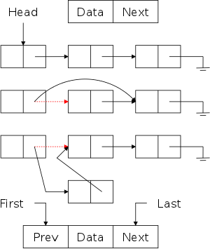
On the right are some pictures. The top row shows a single-linked list node. In addition to the data component (the only content of an array-based list), there is a next component that (somehow, how?) refers to the next node.
The second row shows 3-element long single-linked list. Note the electrical ground symbol that is used to indicate a null reference. To access the list, a reference to the head is stored and, from this reference, the entire list can be found by following next references.
The third row shows the actions needed to delete a node (in this case the center node) from the top list. Note that to delete the center node we need to alter the next component of the previous node and thus need a reference to this node. Thus, given just a reference to a node (and the list head), deletion is a Θ(N) operation, with the most effort needed to find the previous node.
The fourth row shows the actions needed to insert a node between the first and second nodes of the top list. This operation requires a reference to the first node, i.e., to the node after which the insertion is to take place.
Finally, the fifth row shows a single node double-linked list.
On the board do the equivalent of the rows 2-4 for a double-linked list.
Lists, sets, bags, queues, dequeues, stacks, etc. all represent collections of elements (with some additional properties). The Java library implementation of these ADTs all implement the Collection interface.
We need to begin by reviewing some Java.
Recall from 101 that an interface is a class having no real methods (they are all abstract) and no true variables (they are all constants, static final in Java-speak).
One interface can extend one or more other interfaces and one class can implement one or more interfaces; whereas a class can extend only one other class.
Typically, an interface specifies a property satisfied by various classes. For example, any class that implements the Comparable interface is guaranteed to provide a compareTo() instance method, which can be used to compare two objects of the class. The idea is that, if obj1.compareTo(obj2) returns a negative/zero/positive integer, then obj1 is less/equal/greater than obj2.
One advantage of having interfaces is that it ensures uniformity. For example, every class that implements Comparable supplies compareTo() rather than compareWith() or comparedTo() or ... .
The Collection interface abstracts the notion of the English word collection: all classes extending Collection contain objects that are collections of elements. What type are these elements?
The Java Collection interface is generic and so it normally written as Collection<E>, the E is a type variable giving the type of the elements (the letter E is used to remind us that the type parameter determines the elements used).
For example, if a class C implements Collection<String> then a C object contains a collection of Strings.
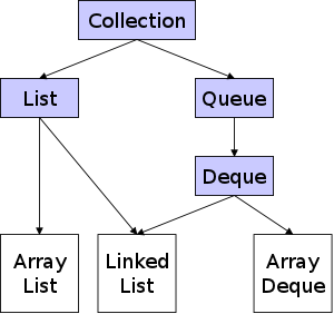
We shall see that there are many kinds of Java collections; indeed the online API shows 10 interfaces and 31 classes in the Collection hierarchy. A very small subset of the hierarchy is shown on the right. Those boxes shown with a light blue background are interfaces; those with a white background are real classes. The longer names are split just for formatting.
Since List is only an interface (not a full class like LinkedList), you can write.
List list1 = new LinkedList(...);
or
LinkedList list2 = new LinkedList(...);
but not
List list3 = new List(...).
Why would you ever want to use list1 instead of
list2?
Because then you would be sure that you are employing only the
List properties of list1.
Thus, if you wanted to switch from a LinkedList
implementation to an ArrayList implementation, you would
need change just the declaration of List1 to
List list1 = new ArrayList(...);
and you are assured that everything else will work unchanged.
Note that a LinkedList IS-A Deque as well as a
List, but by using list1, you can be sure that you
are not using any Deque methods.
Since Collection is the root of the hierarchy, all the components of the Collection interface are available in the 10 other interfaces in the hierarchy as well as the 31 classes.
public interface Collection <E> extends Iterable<E> {
  int size();
  boolean isEmpty();
  boolean contains();
  void clear();                     // destructive
  boolean add(Object o);            // destructive
  boolean remove(Object o);         // destructive
  java.util.Iterator<E> iterator();
  // 9 others
}
The Collection interface includes a number of simple methods.. For example, size() returns the number of elements currently present, contains() determines if an element is present, and isEmpty() checks if the collection is currently empty.
The above methods only query the collection, they do not modify it.
Other methods in Collection actually change the collection
itself.
Apparently, these are called destructive
, but I don't believe
that is a good name since in English destroy
suggests
delete
or at least render useless
, which overstate
mere modifications.
Three of these destructive methods are clear(), which
empties the collection, add(), which inserts, and
remove(), which deletes.
Remark: I find the following material on the Iterable<E> and Iterator interfaces and the associated methods (one of which is iterator()) to be unmotivated at this point so will study the material in a slightly different order. We will skip to 3.3.3 and come back here after 3.4. At that point I believe it is much easier to motivate.
In fact Collection is itself a subinterface of Iterable (which has no superinterface). The later interface supports the for-each loops, touched upon briefly in 101 for arrays.
Recall from 101 that Java has a for-each construct that permits one to loop sequentially through an array examining (but not changing) each element in turn.
for(int i=0; i<a.length; i++) {   |  for(double x: a) {
  use (NOT modify) a[i]           |    use (NOT modify) x
}                                 |  }
Assume that a has been defined as an array of doubles.
Then instead of the standard for loop on the near right,
we can use the shortened, so-called for-each
variant on the
far right.
public class Test {
  public static <E> void f(Iterable<E> col) {
    int count=0;
    for (E i : col)
      count++;
  }
}
This interface guarantees the existence of a for-each loop for objects. Thus any class that implements Iterable provides the for-each loop for its objects, analogous to the for-each taught in 101 for arrays. This is great news for any user of the class; but is an obligation for the implementor of the class.
The trivial code on the right shows how to count the number of elements in any Interable object.
Since Collection extends Iterable, we can use a for-each loop to iterate over the elements in any collection.
But what if you wanted a more general loop, say a while loop or what if you want to remove some of the elements? Lets look a little deeper
The Iterable<T> interface also supplies an iterator() method that when invoked returns an Iterator<T> object. This object has three methods: next(), which returns the next element in T; hasNext(), which specifies if there is a next element; and remove(), which removes the element returned by the last next().
Given the first two methods it is not hard to see how the for-each is implement by Java.
Note that remove() can be called at most once per call to next() and that it is illegal (and gives unspecified results) if the Collection is modified during an iteration in any way than by remove().
The List interface extends Collection and so has more stuff (constants, methods) specified. If you are a user of a class that implements List (such as ArrayList or LinkedList) this is good news: there is more available for you to use.
If, on the other hand you are an implementor of a class that is required to extend List, this is bad news. There is more for you to implement.
At different times we will take on both roles. For now we are users so we are anxious to find out what goodies are available that weren't available for Collection.
Note that the real section heading should be
The List<E> Interface, and the
ArrayList<E>, and LinkedList<E>
(Classes)
.
Although we will write Java that does use the type parameter, for a
while will not emphasize it.
The fundamental concept that List adds to Collection is that the elements in a list are ordered. That is a list, unlike a collection, has a concept of first element, a 25th element, etc.. Note that this is not a size ordering as you can have a list of Integers such as {10, 20, 10, 20}, which is clearly not in size ordering (for any definition of size).
public interface List<E> extends Collection<E> {
  E get(int index);
  E set(int index, E element);
  void add(int index, E element);
  E remove(int index);       // book has void not E
  ListIterator<E> listIterator(int index);
}
The code on the right illustrates some of the consequences of this ordered nature. We notice that add() and remove() now include an index parameter, specifying the position at which the method performs its insertion or removal. Naturally the one-argument add() from Collection is also available. The List specification states that this add(), for a List, will insert at the end, where it is fast. (The specification for Collection just states that, after add() is executed, the element is there. So if it was there already, a second instance may or man not be added). We can also get() and set() the element at a given position.
Start Lecture #6
import java.util.*;
public class DemoMakeSumList {
  private static final int LIST_SIZE = 200000;
  public static void main (String[]args) {
    // One or the other of the next 2 declarations
    List<Long> list = new ArrayList<Long>();
    List<Long> list = new LinkedList<Long>();
    // One of the other of the next 2 method calls
    makelist1(list, LIST_SIZE);
    makelist2(list, LIST_SIZE);
    System.out.println(sum(list));
  }
  public static void makeList1(List<Long> list, int N) {
    list.clear();
    for (long i=0; i<N; i++)
      list.add(i);       // insert at the end
  }
  public static void makeList2(List<Long> list, int N) {
    list.clear();
    for (long i=0; i<N; i++)
      list.add(0,i);     // insert at the beginning
  }
  public static int sum(List<Long>, list) {
    int ans = 0;
    for (int i=0; i<list.size(); i++);
      ans += list.get(i);
    return ans;         // missing in book
  }
}
We will see two implementations of the List interface: ArrayList and LinkedList. The code on the right illustrates how they can be used.
The important item to note is that only the declaration of list changes; the rest of the program stays exactly the same. However, the performance of the list operations does change.
As expected ArrayList uses a (dynamically resizeable) array to store the list. This makes retrieving an item from a known position very fast (O(1), i.e., constant time). Thus executing sum() is quite fast (O(N)). The bad news is that inserting and removing items are slow (O(N), i.e., linear time) unless the item is near the end of the list. Thus executing makeList1() is fast (O(N)), but executing makeList2 is slow (O(N2)).
The LinkedList implementation uses a double-linked list as we pictured above. This makes all insertions and deletions O(1) (provided we know the position at which to operate, or are operating at an index near an end). Thus both makeList1() and makeList2() are fast (O(N). However, getting and setting by index are O(N) (unless the index is near one of the ends). Thus sum() is slow (O(N2)).
Consider the problem of removing every even number from a List of Longs. Note that no (reasonable) implementation of remove() can make the code efficient if list is actually an ArrayList, but we can hope for a fast implementation if list is a LinkedList.
public static void removeEvens1(List<Long> list) {
  int i = 0;
  while (i < list.size())
    if (list.get(i) % 2 == 0)
      list.remove(i);
    else
      i++;
}
A straightforward solution using the index nature of a List is shown on the right. This does indeed work, but stepping through a list by index guarantees poor performance for a LinkedList, the one case we had hopes for good performance. The trouble is that we are using the same code to march through list and this code is good for one List implementation and poor for the other. The right solution uses iterators, which we are downplaying for now.
public static void removeEvens2(List<Long> list) {
  for (Long x: list)
    if (x % 2 == 0)
      list.remove(x);
}
Given the task of removing all even numbers from a
List<Long>, a for-each
would appear
to be perfect, slick, and best of all easy; a trifecta.
Since List extends Iterable, a List
object such as list can have all its elements accessed
via a for-each
loop, with the benefit that the low level
code will be tailored for the actual class of list
(ArrayList or LinkedList).
The code is shown on the right.
Unfortunately, we actually hit a tetrafecta: perfect, slick,
easy, and wrong!
The rules involving for-each
loops, whether for arrays or
for Iterable classes, forbid modifying the array or
collection during loop execution.
public static void removeEvens3(List<Long> list) {
  Iterator<Long> iter = list.iterator();
  while (iter.hasNext())
    if (iter.next() % 2 == 0)
      iter.remove();
}
The solution is to write the loop ourselves using the hasNext() and next() methods of the Iterator. We then use the remove() method of the Iterator to delete an element if it is even. Note that this remove() is not the same method mistakenly used above. This one is from the Iterator class; the previous one was from the List class. Also note that remove() is called at most once after each call of next(). This is required! The correct code is on the right.
A ListIterator, unlike a mere Iterator found in a Collection can retrieve either the next or previous element.
Specifically, an instance of ListIterator has the additional methods hasPrevious() and previous(). Moreover, remove() may now be called once per call to either next() or previous() and it removes the element most recently returned by next() or previous().
Lab 1, Part 4 (the last part) assigned. Due 1 March 2011.
As mentioned previously we will look at lists from three viewpoints:
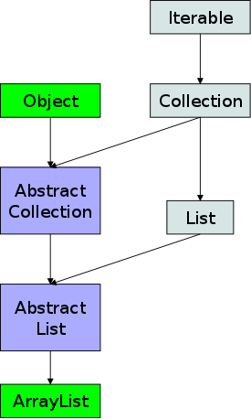
The Java library has excellent list implementations, which as we
have seen, form a fairly deep hierarchy.
For example, the diagram on the right shows the classes (green),
abstract classes (dark blue), and interfaces (light blue) that
lie above
ArrayList in the hierarchy.
The abstract classes serve as starting points for user written classes. They implement some of the methods in the interface.
We cannot hope to match the quality of this high-class implementation and if one needed to use an ArrayList, I would strongly recommend the library class and not the one we will develop, whose purpose is to better understand how to implement a list as an array.
We will be content to just implement a version of ArrayList that we will call MyArrayList and will not reproduce any of the hierarchy.
void clear();
int size();
boolean isEmpty();
E get(int index);
E set(int index, E element);
boolean add(Object o);
void add(int index, E element);
E remove(int index);
boolean remove(Object o);
boolean contains();
Iterator<E> iterator();
To implement ArrayList we need to implement all the methods in List. Since List extends Collection, which extends Iterable, we need to implement all of those methods as well.
If we wrote our ArrayList as an extension of AbstractList this task would be fairly easy since the latter implements most of the needed methods. However, we are working from scratch.
Looking back to our discussions of Collection and List we see that our task is to implement the methods on the right. Both classes have other methods as well; we will be content to implement these.
One simplification we are making, at least initially, is to ignore Iterable. I have removed those portions from the code below, which is an adaptation of figures 3.15 and 3.16.
public class MyArrayList<E>
             implements Iterable<E> {


  private static final int DEFAULT_CAPACITY=10;
  private int theSize;
  private E[] theElements;


  public MyArrayList() {
    clear();
  }

  public void clear() {
    theSize = 0;
    ensureCapacity(DEFAULT_CAPACITY);
  }


  private void ensureCapacity(int newCapacity) {
    if (newCapacity < theSize)
      return;
    E[] old = theElements;
    theElements = (E[]) new Object[newCapacity];
    for (int i=0; i<size(); i++)
      theElements[i] = old[i];
  }


  public int size() {
    return theSize;
  }

  public boolean isEmpty() {
    return size() == 0;
  }


  public E get(int index) {
    if (index < 0 || index >= size())
      throw new ArrayIndexOutOfBoundsException();
    return theElements[index];
  }

  public E set(int index, E newVal) {
    if (index < 0 || index >= size())
      throw new ArrayIndexOutOfBoundsException();
    E old = theElements[index];
    theElements[index] = newVal;
    return old;
  }


  public boolean add(E x) {
    add(size(), x);
    return true;
  }

  public void add(int index, E x) {
    if (theElements.length == size())
      ensureCapacity(size() * 2 + 1);
    for (int i=theSize; i>index; i--)
      theElements[i] = theElements[i-1];
    theElements[index] = x;
    theSize++;
  }


  public E remove(int index) {
    E removedElement = theElements[index];
    for (int i=index; i<size()-1; i++)
      theElements[i] = theElements[i+1];
    theSize--;
    return removedElement;
  }

  public boolean remove (Object o) {
    // part of lab 2
  }


  public boolean contains(Object o) {
    for (int i=0; i<size(); i++) {
      E e = theElements[i];
      if ( (o==null) ? e==null : o.equals(e) )
        return true;
    }
    return false;
  }


// ignore the rest for now
  public java.util.Iterator<E> iterator() {
    return new ArrayListIterator<E>(this);
  }
  private static class ArrayListIterator<E>
          implements java.util.Iterator<E> {
  }
}
The first thing to notice is that MyArrayList is generic and that the elements in the list are of type E. You can think of E as Integer (but NOT int), or String, or even Object.
As written MyArrayList does not implement List. To do so would require implementing a whole bunch of methods, which will be done when we revisit this class later.
The class contains two data fields theElements, the actual array used to store the elements and theSize, the current number of elements. Note that theSize is not theElements.lenght, we refer to the later as the capacity and the code makes use of the auxiliary method ensureCapacity(), discussed below, to keep the capacity of the array large enough to contain theSize elements. There is also a symbolic constant DEFAULT_CAPACITY.
All of these are declared private since we do not want clients (i.e., users) of our lists to access these items.
There is just one (no-arg) constructor. Please be sure you recall from 101 the situation when the constructor is executed: The data fields are already declared, but they are not initialized. For theSize this is clear, we have an uninitialized int. For the array theElements it means that the variable exists, but does not yet point to an array. The latter is the job of clear(), which uses the helper method ensureCapacity() to set theElements() to an initialized array capable of holding DEFAULT_CAPACITY elements (but currently holding none).
This method, using the technique in 3.2.1, changes the capacity of the array, but never to a value less than the current size of the list. As a helper functions, ensureCapacity() is naturally private. I don't know why the book has it public.
These methods are given an index at which to operate. Naturally, get() returns the value found and wisely set() returns the old value, which can prove useful. Both methods raise an exception if the index is out of bounds, which seems inconsistent since add() and remove() do not make the corresponding check.
Collection specifies an add() method with one parameter, an element, which is added somewhere to the collection. List refines this specification to require that the element is added at the end. List also specifies an additional add() with a 2nd parameter giving the position to add the element.
The second method is implemented by moving forward all the elements from that position onward and then inserting into the resulting hole. The first method is implemented as a special case of the second.
If the List is full prior to the insertion, its size is first doubled via ensureCapacity().
The remove() added to Collection by List is fairly simple. It removes and returns the element at the specified index, sliding down any succeeding elements. The size is adjusted.
The remove in Collection is given an element and returns a boolean indicating whether the element is present in the list. If it is present, one occurrence is removed. List strengthens this specification to require that, if the element is present, the first occurrence is removed.
This second method will be part of lab 2.
The textbook has the parameter as E, the Java specification states Object. The book has no implementation (actually it is an exercise). The at first strange looking code on the right is essentially straight from the specification. Let us look at the specification for contains() and see how it gives rise to the code on the right. This is a useful skill since it is the key to effective use of the Java library.
We are skipping this part now; it will be discussed later.
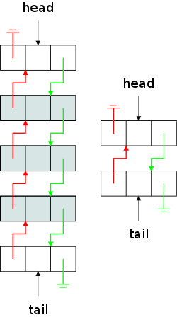
Early in the chapter we sketched a double linked list just to show
the forward and backward links.
It turns out to be easier to program such lists (fewer special
cases) if the two end nodes are not used for data but as special
head
and tail
nodes.
As a result the diagram on the near right represents a list with
only three elements, the shaded nodes.
As before, we use the electrical ground
symbol to represent a
null reference.
The green arrows are the next references and the red arrows
are the prev references.
The middle component is the data.
Since we are implementing List<E>, the type of the
data is E.
Assuming the list is not empty, the first element of the list is
(the central data component of) head.next and the last
element is tail.prev.
An empty double linked list, an example of which is drawn on the far right, would therefore have two nodes that point to each other as well as to ground. Those are the same two that were unshaded in the near right diagram. For an empty list tail.prev==head and head.next==tail.
Our task is basically the same as with ArrayList: We need to implement the List interface, whose methods are repeated on the right. Naturally, the implementation is different and the corresponding methods will have different performance in the two List implementations.
void clear();
int size();
boolean isEmpty();
E get(int index);
E set(int index, E element);
boolean add(Object o);
void add(int index, E element);
boolean remove(Object o);
E remove(int index);
boolean contains();
One significant implementation difference is that the basic data structure in the ArrayList implementation is an array, which is already in Java. For LinkedList we need, in addition to a few variables, an unbounded number of nodes (N+2 nodes for a list with N elements).
So we need two classes MyLinkedList and MyNode. The former class will have all the methods as well as the two nodes constituting an empty list, the latter class just contains the three data fields that comprise a node. Two of these fields (prev and next) should be knowable only to the two classes. In particular they should be hidden from the users of these classes.
The right
way to do this is to have the MyNode class
defined inside the MyLinkedList class and we will do this
eventually.
For now to avoid taking a time out to learn about nested (and inner)
classes we will make both classes top level, understanding that this
does not hide prev and next as well as we
should.
Start Lecture #7
public class Node<E> {
  public E data;
  public Node<E>   prev;
  public Node<E>   next;

  public Node(E d, Node<E> p, Node<E> n) {
    data=d; prev=p; next=n;
  }
}
The node class looks easy. It has three fields and a constructor that initializes them to the given arguments.
But wait it looks impossible!
How can a node contain two nodes (and something else).
Is this magic or a typo?
Neither, it's an old friend, reference semantics.
As written this class implements neither List nor Iterable. We shall revisit MyLinkedList and enhance the implementation so that List and Iterable are indeed implemented.
public class MyLinkedList<E> {
  private int theSize;
  private Node<E> beginMarker;
  private Node<E> endMarker;

  public MyLinkedList() {
    clear();
  }

  public void clear() {
    beginMarker = new Node<E>(null, null, null);
    endMarker = new Node<E>(null, beginMarker, null);
    beginMarker.next = endMarker;
    theSize = 0;
  }


  public int size() {
    return theSize;
  }

  public boolean isEmpty() {
    return size() == 0;
  }


  public E get(int index){
    return getNode(index).data;
  }

  private Node<E> getNode(int index) {
    Node<E> p;
    if (index<0 || index>size())
      throw new IndexOutOfBoundsException();
    if (index < size()/2) {
      p = beginMarker.next;
      for (int i=0; i<index; i++)
    p = p.next;
    } else {
      p = endMarker;
      for (int i=size(); i>index; i--)
    p = p.prev;
    }
    return p;
  }

  public E set(int index, E newVal) {
    Node<E> p = getNode(index);
    E oldVal = p.data;
    p.data = newVal;
    return oldVal;
  }


  public void add(int index, E x) {
    addBefore(getNode(index), x);
  }

  public boolean add(E x) {
    add(size(), x);
    return true;
  }

  private void addBefore(Node<E> p, E x) {
    Node<E> newNode = new Node<E>(x, p.prev, p);
    newNode.prev.next = newNode;
    p.prev = newNode;
    theSize++;
  }


  public E remove(int index) {
    return remove(getNode(index));
  }

  private E remove(Node<E> p) {
    p.next.prev = p.prev;
    p.prev.next = p.next;
    theSize--;
    return p.data;
  }


  public boolean remove(Object o) {
    // part of lab 2
  }
}
There are just three fields, the two end nodes present in any list and the current size of the list.
The constructor just uses clear() to produce an empty list. Show, on the board show that clear() does produce our picture.
Note that if clear is employed by the user to clear a nonempty
list, the original nodes are just left hanging around.
A bug?
No.
Garbage collection will retrieve them.
The get() method, which was straightforward with the array-based implementation, is harder this time. The difficulty is that we are given an index as an argument, but a linked list, unlike an array-based list, does not have indices.
Pay attention to the getNode() helper (i.e., private) method, which starts at the nearest end and proceeds forward or backward (via next or prev) until it arrives at the appropriate node. This node can be the end marker, but not the begin marker.
The set() method uses the same helper to find the node in question. Note that set returns the old value present, which can prove very useful.. Pay particular attention to the declarations without a new operator and remember reference semantics.
Specifically, the declaration of p does not create a new node. It just creates a new node variable and initializes this variable to refer to an existing node. Similarly the declaration of oldVal does not create a new element (a new E), but just a new element variable.
The add() specified in List is given an index as well as an element and is to add a node with this element so that it appears at the given index. This implies that it must be inserted before the node currently at that index. The task is accomplished using two helpers: getNode(), which we have already seen, and addBefore (see below), which does the actual insertion.
The add() specified in Collection just supplies the element, which may be inserted anywhere. The List specification refines this to require the element be added at the end of the list. Therefore, this method simply calls the other add() giving size() as the insertion site.
Thanks to getNode(), addBefore() is given an element and a node before which it is to add this element. Show the pointer manipulation on the board.
The List remove() is given an index and removes the corresponding node (found by getNode()). Draw pictures on the board to show that the code (in the helper remove() method) is correct.
Analogous to the situation with add(), the Collection remove(), specifies that an occurrence of the argument Object be removed and the List spec refines this to the first occurrence.
This remove() will be part of lab 2.
List<Long> list;   // Maybe Array or maybe Linked
...
Long sum = 0;
for (int i=0; i<list.size(); i++)
  sum += list.get(i);
We have now seen the implementation for two different implementations of the List interface. For either one we can sum the elements as shown on the right. It is great that the exact same code can be used for either implementation.
What is not great is that the code used is very efficient for an ArrayList, but is quite inefficient for a LinkedList. See the timing comparison below.
The problem is that when we change list from
ArrayList to LinkedList, the methods change
automatically, but the looping behavior does not change ...
... until now.
A for loop is tailor made for an array, but is inappropriate for a linked structure. The solution is to use a more generic loop made from the three parts of a for: initialization, test, advance-to-next.
The initialization is done as a special case of advance-to-next. What is needed are methods to test for completion and to advance to the next (or first) element of the List (actually this works for any Collection, really for any Iterable<E>). These methods are called hasNext() and next() respectively.
public class DemoMakeSumList {
  private static final int LIST_SIZE = 20;
  public static void main (String[]args) {
    //List<Long> list = new ArrayList<Long>();
    List<Long> list = new LinkedList<Long>();
    //makeList1(list, LIST_SIZE);
    makeList2(list, LIST_SIZE);
    System.out.println(sum(list));
  }
  public static void makeList1(List<Long>list,
                               int N) {
  list.clear();
  for (long i=0; i<N; i++)
    list.add(i);       // insert at the end
  }
  public static void makeList2(List<Long>list,
                               int N) {
    list.clear();
    for (long i=0; i<N; i++)
      list.add(0,i);     // insert at beginning
  }
  public static long sum(List<Long> list) {
    long ans = 0;
    for (int i=0; i<list.size(); i++)
      ans += list.get(i);
    return ans;        //  missing in book
  }
}
On the right is code we saw previously that makes and sums a list of Longs. Note that the code for sum() uses list.get() for each index in the loop, a great plan for ArrayList, but a poor technique for LinkedList.
The code below shows sum() rewritten to use hasNext() and next().
public static long sum(List<Long> list) {
  long ans = 0;
  Iterator<Long> iter = list.iterator();
  while (iter.hasNext())
    ans += iter.next();
  return ans;
}
Compare the above with using a Scanner. We declare and create (with new) a Scanner instance (I normally call mine getInput) and then to get the next (or first) String, I use getInput.next(). To find if there is another String, I use getInput.hasNext().
The Iterator (really Iterator<E>) interface abstracts this next/hasNext idea. Indeed, the Scanner class implements Iterator<String>
The List interface does not extend Iterator so the code above could not say list.next(). Instead, List extends (Collection, which extends) the Iterable interface. Thus, any class implementing List, must implement Iterable. Iterable specifies a parameterless method iterator(), which returns an Iterator. That is how the code above created iter. Like any Iterator, iter contains instance methods next(), hasNext(), and remove(), the first two of which are used above.
public static long sum(List<Long> list) {
  long ans = 0;
  for (long x: list)
    ans += x;
  return ans;
}
We have just seen that, if a class implements Iterable
(not Iterator), then each instance of the class can create
an Iterator, which contains next() and
hasNext() methods.
This permits the loop we just showed.
The extra goody is that the Java compiler permits a more pleasant
syntax to be used in this case, the for-each
loop that we saw
in 101 for arrays.
It is shown on the right.
(Offering an alternative nicer
syntax, is often called
syntatic sugaring
.
import java.util.*;
public class DemoMakeSumList {
  private static Calendar cal;
  private static final int LIST_SIZE = 200000;
  public static void main (String[]args) {
    long sum;
    List<Long> list1 = new ArrayList<Long>();
    List<Long> list2 = new LinkedList<Long>();
    printTime("Start Time (ms):       ");
    makeList1(list1, LIST_SIZE);
    printTime("Made ArrayList at end: ");
    makeList2(list1, LIST_SIZE);
    printTime("Made ArrayList at beg: ");
    sum = sum1(list1);
    printTime("Sum ArrayList std for: ");
    System.out.println("  " + sum);
    sum = sum2(list1);
    printTime("Sum ArrayList foreach: ");
    System.out.println("  " + sum);
  }
  public static void printTime(String msg) {
    cal = Calendar.getInstance();
    System.out.println(msg + cal.getTimeInMillis());
  }
  public static void makeList1(List<Long>list,int N) {
  list.clear();
  for (long i=0; i<N; i++)
    list.add(i);       // insert at the end
  }
  public static void makeList2(List<Long>list,int N) {
    list.clear();
    for (long i=0; i<N; i++)
      list.add(0,i);     // insert at the beginning
  }
  public static long sum1(List<Long> list) {
    long ans = 0;
    for (int i=0; i<list.size(); i++)
      ans += list.get(i);
    return ans;        //  missing in book
  }
  public static long sum2(List<Long> list) {
    long ans = 0;
    for (long x: list)
      ans += x;
    return ans;
  }
}
On the right is the beginnings of an attempt to actually time the results of the various versions of list, makeList(), and sum()
The Calendar class seems to be the way to get timing information. See my printTime() on the right. After declaring a Calendar you can initialize it using Calendar.getInstance() and then find the number of milliseconds (a long) since the Epoch (Midnight GMT, 1 January 1970) by invoking getTimeInMillis().
The output of the code on the right is as follows.
Start Time (ms):       1297877874798
Made ArrayList at end: 1297877874816
Made ArrayList at beg: 1297877879840
Sum ArrayList std for: 1297877879849
  19999900000
Sum ArrayList foreach: 1297877879860
  19999900000
We see that making an ArrayList by inserting at the end
required 0.018 seconds, but inserting at the beginning raised that
to 5.024 seconds.
Summing this list with a for loop took 0.009 seconds and
with a for-each
loop 0.011 seconds.
Certainly this could be presented better, and what about the other
half, i.e., using the LinkedList list2?
Answer: That will be (an easy) part of lab 2.
For example your version will do the subtractions that we had to do mentally to figure out how long each step required. Also dividing by 1000 and using something like "%6.3f" as a format, would give seconds rather than milliseconds.
But this timing data should not obscure the important point that to change from an ArrayList to a LinkedList requires us to change the declaration and nothing else.
Homework:
Add main() methods to each of our two
List implementations, MyArrayList and
MyLinkedList.
The main() methods should be essentially identical.
Each should create one or more lists (that is the difference, one
will say Array
where the other says Linked
).
The add a few elements, do some gets and sets, maybe a remove.
In general exercise the methods of the classes.
Note that except for the list declarations and creations, the two
main programs should be character for character the same.
Start Lecture #8
Homework: 3.1, 3.2.
Remark: Now we can go back and explain much of the previously gray'ed out material. I have given a light green background to those parts of the notes that appeared previously.
In fact Collection is itself a subinterface of Iterable (which has no superinterface). The later interface supports the for-each loops, touched upon briefly in 101 for arrays.
Recall from 101 that Java has a for-each construct that permits one to loop sequentially through an array examining (but not changing) each element in turn.
for(int i=0; i<a.length; i++) {   |  for(double x: a) {
  use (NOT modify) a[i]           |    use (NOT modify) x
}                                 |  }
Assume that a has been defined as an array of doubles.
Then instead of the standard for loop on the near right,
we can use the shortened, so-called for-each
variant on the
far right.
This interface guarantees the existence of a for-each loop for objects. Thus any class that implements Iterable provides the for-each loop for its objects, analogous to the for-each taught in 101 for arrays. This is great news for any user of the class; but is an obligation for the implementor of the class.
public class Test {
  public static <E> void f(Iterable<E> col) {
    int count=0;
    for (E i : col)
      count++;
  }
}
The generic method on the right counts the number of elements in any Interable object. The first <E> tells Java that E is a type parameter. Were it omitted, the compiler would think that the second E is an actual type (and would print an error since there is no such type).
Since List extends Collection, which extends Iterable, we can use a for-each loop to iterate over the elements in any Collection (in particular any List).
But what if you wanted a more general loop, say a while loop or what if you want to remove some of the elements? Let's look a little deeper.
The Iterable<T> interface specifies an iterator() method that when invoked returns an Iterator<T> object. This object has three instance methods: next(), which returns the next element in T; hasNext(), which specifies if there is a next element; and remove(), which removes the element returned by the last next().
Given the first two methods it is not hard to see how the for-each is implement by Java.
Note that remove() can be called at most once per call to next() and that it is illegal (and gives unspecified results) if the Collection is modified during an iteration in any way other than by remove().
Consider the problem of removing every even number from a List of Longs. Note that no (reasonable) implementation of remove() can make the code efficient if list is actually an ArrayList, but we can hope for a fast implementation if list is a LinkedList.
public static void removeEvens1(List<Long> list) {
  int i = 0;
  while (i < list.size())
    if (list.get(i) % 2 == 0)
      list.remove(i);
    else
      i++;
}
A straightforward solution using the index nature of a List is shown on the right. This does indeed work, but stepping through a list by index guarantees poor performance for a LinkedList, the one case we had hopes for good performance. The trouble is that we are using the same code to march through any kind of list and this code is good for one List implementation and poor for the other.
public static void removeEvens2(List<Long> list) {
  for (Long x: list)
    if (x % 2 == 0)
      list.remove(x);
}
Given the task of removing all even numbers from a
List<Long>, a for-each
solution would appear
to be perfect, slick, and best of all easy; a trifecta.
Since List extends Iterable, a List
object such as list can have all its elements accessed
via a for-each
loop, with the benefit that the low level
code will be tailored for the actual class of list
(ArrayList or LinkedList).
The code is shown on the right.
Unfortunately, we actually hit a tetrafecta: perfect, slick,
easy, and wrong!
The rules involving for-each
loops, whether for arrays or
for Iterable classes, forbid modifying the array or
collection during loop execution.
public static void removeEvens3(List<Long> list) {
  Iterator<Long> iter = list.iterator();
  while (iter.hasNext())
    if (iter.next() % 2 == 0)
      iter.remove();
}
The solution is to write the loop ourselves using the hasNext() and next() methods of the Iterator. We can then use the remove() method of the Iterator to delete an element if it is even. Note that this remove() is not the same method mistakenly used above. This one is from the Iterator class; the previous one was from the List class. Also note that remove() is called at most once after each call of next(). This is required! The correct code is on the right.
A ListIterator, unlike a mere Iterator found in a Collection can retrieve either the next or previous element.
Specifically, an instance of ListIterator has the additional methods hasPrevious() and previous(). Moreover, remove() may now be called once per call to either next() or previous() and it removes the element most recently returned by next() or previous().
public class MyArrayList<E>
             implements Iterable<E> {
  private static final int DEFAULT_CAPACITY=10;
  private int theSize;
  private E[] theElements;
  public MyArrayList() {
    clear();
  }
  public void clear() {
    theSize = 0;
    ensureCapacity(DEFAULT_CAPACITY);
  }
  private void ensureCapacity(int newCapacity) {
    if (newCapacity < theSize)
      return;
    E[] old = theElements;
    theElements = (E[]) new Object[newCapacity];
    for (int i=0; i<size(); i++)
      theElements[i] = old[i];
  }
  public int size() {
    return theSize;
  }
  public boolean isEmpty() {
    return size() == 0;
  }
  public E get(int index) {
    if (index < 0 || index >= size())
      throw new ArrayIndexOutOfBoundsException();
    return theElements[index];
  }
  public E set(int index, E newVal) {
    if (index < 0 || index >= size())
      throw new ArrayIndexOutOfBoundsException();
    E old = theElements[index];
    theElements[index] = newVal;
    return old;
  }
  public boolean add(E x) {
    add(size(), x);
    return true;
  }
  public void add(int index, E x) {
    if (theElements.length == size())
      ensureCapacity(size() * 2 + 1);
    for (int i=theSize; i>index; i--)
      theElements[i] = theElements[i-1];
    theElements[index] = x;
    theSize++;
  }
  public E remove(int index) {
    E removedElement = theElements[index];
    for (int i=index; i<size()-1; i++)
      theElements[i] = theElements[i+1];
    theSize--;
    return removedElement;
  }
  public boolean remove (Object o) {
    // part of lab 2
    return true;  // so that it compiles
  }
  public boolean contains(Object o) {
    for (int i=0; i<size(); i++) {
      E e = theElements[i];
      if ( (o==null) ? e==null : o.equals(e) )
        return true;
    }
    return false;
  }
  public java.util.ListIterator<E> iterator() {
    return new ArrayListIterator<E>(this);
  }
  private static class ArrayListIterator<E>
          implements java.util.ListIterator<E> {
    private int current = 0;
    private MyArrayList<E> theList;
    public ArrayListIterator(MyArrayList<E> list) {
      theList = list;
    }
    public boolean hasNext() {
      return current < theList.size();
    }
    public E next() {
      return theList.theElements[current++];
    }
    public void remove() {
      theList.remove(--current);
    }
    public int nextIndex() {
      return current;
    }
    public boolean hasPrevious() {
      return current > 0;
    }
    public E previous() {
      return theList.theElements[--current];
    }
    public int previousIndex() {
      return current-1;
    }
    public void add(E e) {
      throw new UnsupportedOperationException();
    }
    public void set(E e) {
      throw new UnsupportedOperationException();
    }
  }
Recall that we haven't yet fulfilled two obligation with respect to the ArrayList class. Our previous version of MyArrayList has no iterator and so does not implement Iterable it is also missing a number of methods needed to implement List.
A new version implementing Iterable is shown on the right; the missing List methods will appear later.
The only changes are at the very end. The one requirement missing is that we need to have an iterator() method that returns an Iterator. Since we are writing MyArrayList from scratch we need to write the Iterator class as well.
We call this class ArrayListIterator and it represents the bulk of the effort.
Since each instance of MyArrayList will need its own iterator, the method iterator() must somehow pass to the class ArrayListIterator the list involved. This task is accomplished by having the iterator() method pass this to the constructor for ArrayListIterator.
Indeed, if we now look at the iterator() method we see that all it does is call the constructor with this as the sole argument. To explain the new (nested) class is a longer story.
The basic idea is simple, we keep an index called
current reflecting the iterators current position and
then, for example, the next() method would be
return theElements[current++]
enhanced to refer to the list in question.
Now comes a subtlety. If we make ArrayListIterator a top-level class in a file named ArrayListIterator.java, then this class would not see the array theElements since the latter is declared private. We could declare the array public but that would be bad since one of those error-prone (or perhaps even malevolent) users of MyArrayList could mess up theElements.
(There are visibilities between public
and private, which would permit the iterator to see the
array.
This would be better than declaring the array public, but
is not as secure as private.
Were there no better solution, we would learn
about packages
and package private
.
However, there is a better solution, which
permits the array to be declared private, so we will use
that.)
The solution is to have the ArrayListIterator class nested inside the MyArrayList class. Then, as with nesting of blocks in Java, everything declared in the outside class (even if private) is visible to the inside class. Names declared private in the inside class are not visible in the outside class.
One more subtlety: Java has two way to nest one class inside
another:
In Java-speak, the inside class can be either a nested
class or an inner
class.
The syntatic distinction is that an nested class uses the keyword
static in its definition; whereas, an inner class does
not.
As you can see our MyArrayListInerator is a nested
class.
The semantics of a nested class is pretty much the same as the semantics in other programming languages that permit nesting. It is also pretty much the same as the Java semantics for nested blocks. (An inner class is more unusual; each instantiation of the inner class is associated with the instantiation of the outer class that executed the new operator on the inner class.) I believe we can avoid inner classes; see the book for more information on their use. In particular, the book uses an inner class for ArrayListIterator.
After all the hoopla, the actual nested class is fairly straightforward. The variable theList refers to the MyArrayList in question. It is set in the constructor (from the argument, which is this) and used in several places. The index current keeps track of where we are in theList.
In fact all the methods are one-liners. For example, next() returns the current element and bumps the index (afterward), prev() first decrements the index and then returns the current element, hasNext() checks if we are at the end and hasPrevious checks if we are at the beginning.
Draw some diagrams on the board showing the operations in action.
Note that the book implements only an Iterator; whereas, the code on the right give a ListIterator. In addition to supplying methods for going backwards, a ListIterator also has a number of extra but optional methods. For these, I took the easy way out (explicitly permitted) and threw an UnsupportedOperationException. In fact remove(), which is also in a plain Iterator, is also optional, but, like the book, I did implement it.
Start Lecture #9
Homework: 3.4.
Remark: We have now finished filling in the blanks
(gray'ed out material) so return to section 3.5,
Implementation of LinkedList
.
The current status is that the basic class is written, but with the
following defects, which we will now proceed to remedy.
Long a;
List list;
list = new MyArrayList<long>();
Iterator iter = list.iterator();
while (iter.hasNext())
  a = iter.next();
Remark:
Draw on the board an animation
of the code on the right.
Each frame
of the animation shows one of the statements in
action (the while is broken down into its constituent
if and goto).
On the board I will superimpose the frames so at each step you will
see the result of all preceding steps (I could not fit all the
frames on the board at once.
End of Remark
public class MyLinkedList<E> implements Iterable<E> {
  private int theSize;
  private Node<E> beginMarker;
  private Node<E> endMarker;

  public MyLinkedList() { clear(); }

  public void clear() {
    beginMarker = new Node<E>(null, null, null);
    endMarker = new Node<E>(null, beginMarker, null);
    beginMarker.next = endMarker;
    theSize = 0;
   }
  public int size()        { return theSize; }
  public boolean isEmpty() { return size() == 0; }

  public boolean add(E x) {
    add(size(), x);
    return true;
  }
  public void add(int index, E x) {
    addBefore(getNode(index), x);
  }
  public E get(int index){
    return getNode(index).data;
  }
  public E set(int index, E newVal) {
    Node<E> p = getNode(index);
    E oldVal = p.data;
    p.data = newVal;
    return oldVal;
  }
  public E remove(int index) {
    return remove(getNode(index));
  }
  private void addBefore(Node<E> p, E x) {
    Node<E> newNode = new Node<E>(x, p.prev, p);
    newNode.prev.next = newNode;
    p.prev = newNode;
    theSize++;
  }
  private E remove(Node<E> p) {
    p.next.prev = p.prev;
    p.prev.next = p.next;
    theSize--;
    return p.data;
  }
  private Node<E> getNode(int index) {
    Node<E> p;
    if (index<0 || index>size())
      throw new IndexOutOfBoundsException();
    if (index < size()/2) {
      p = beginMarker.next;
      for (int i=0; i<index; i++)
    p = p.next;
    } else {
      p = endMarker;
      for (int i=size(); i>index; i--)
    p = p.prev;
    }
    return p;
  }
  public boolean remove (Object o) {
    // part of lab 2
    return true;  // so that it compiles
  }
  public boolean contains (Object o) {
    // part of lab 2
    return true;  // so that it compiles
  }
  private static class Node<E> {
    public E data;
    public Node<E>   prev;
    public Node<E>   next;

    public Node(E d, Node<E> p, Node<E> n) {
      data=d; prev=p; next=n;
    }
  }
  public java.util.ListIterator<E> listIterator() {
    return new LinkedListIterator<E>(this);
  }
  private static class LinkedListIterator<E>
                 implements java.util.ListIterator<E> {
    private MyLinkedList<E> theList;
    private Node<E> current;
    public LinkedListIterator(MyLinkedList<E> list) {
      theList = list;
      current = theList.beginMarker.next;
    }
    public boolean hasNext() {
      return current != theList.endMarker;
    }
    public E next() {
      E nextData = current.data;
      current = current.next;
      return nextData;
    }
    public void remove() {
      theList.remove(current.prev);
    }
    public int nextIndex() {
      return getIndex(current);
    }
    private int getIndex(Node p) {
      Node q = theList.beginMarker.next;
      for(int index=0; ; index++) {
    if (p == q)
      return index;
    q = q.next;
      }
    }
    public boolean hasPrevious() {
      return current != theList.beginMarker.next;
    }
    public E previous () {
      E prevData = current.prev.data;
      current = current.prev;
      return prevData;
    }
    public int previousIndex() {
      return getIndex(current.prev);
    }
    public void add(E e) {
      throw new UnsupportedOperationException();
    }
    public void set(E e) {
      throw new UnsupportedOperationException();
    }
  }
}
The only substantive changes to MyLinkedList are nesting the Node class inside MyLinkedList and implementing the LinkedListIterator (also as a nested class). For completeness, however, the entire MyLinkedList class appears on the right.
Since we have learned about nested classes and have used one in MyArrayList, it will not be hard to do the same for MyLinkedList, as we shall now see.
The code on the right still does not implement all the methods to be a full implementation of List. This was also true of MyLinkedList. As a result, neither of the following Java statements will compile.
    List list<Long> list =
         new MyArrayList<Long>();
    List list<Long> list =
         new MyLinkedList<Long>();
Since we want to use our implementation with Lists, I have extended our two implementations to add all the other methods, often by suppling non-functioning stubs. Since we will not invoke those extra methods, the stubs are adequate. Both classes and a trivial test program can be found here. Note that as promised earlier the code using list is identical for both implementations.
A LinkedList, just like an ArrayList, should have the List-enhanced version of the remove() method found in Container.
This will be part of Lab 2
A LinkedList, just like an ArrayList, should have a contains() method. This will another part of Lab 2.
This is simple (now that we know how to do it!). Just move the Node class inside and make it private static.
The advantages obtained from using a nested class instead of an additional top-level class as in our previous implementation include
As was the case with MyArrayList, implementing the ListIterator requires two components: a listIterator() method and a class LinkedListIterator<E>. Once again, the first is quite easy; the second requires more work.
Indeed the listIterator() method is essentially the same as for MyArrayList.
The new class, as with MyArrayList needs to keep a reference to the list in question. This is stored in theList which is set in the constructor. The constructor is again called with an argument of this.
Also repeated from MyArrayList is a variable current, which is now a reference to the next Node (i.e., the Node whose data component would be return by the next() method). For MyArrayList, the corresponding variable is an index and thus can be initialized to zero in the declaration. Here current is initialized to the successor of beginMarker (which is a reference to either the first Node of the list or to the endMarker, if the list is empty).
This latter initialization must be performed in the constructor
after theList has been initialized, as I learned
the hard way
.
The individual methods hasNext(), hasPrevious(), etc. are reasonably straightforward. However, we are not as familiar with linked structures as we are with arrays, so we should draw pictures on the board to see how they work.
If we gave the MyArrayList and MyLinkedList a
reasonable amount of testing and fixed all the obvious bugs, how
would we rate the result?
I would give them a B / B-.
They are functional but ...
Homework: 3.8
From a computer science (not a Java) point of view a stack is list with restrictions, namely all insertions and all deletions are done at the end of the list. In particular it is not possible to insert or deleted in the middle.
The three fundamental operations (methods) that can be performed on a stack are push(), pop(), and top.
The common terminology is to refer to the end of the stack as its top. I believe the origin of this terminology is from a stack of real world objects, e.g., dishes. Then adding a dish to the stack of dishes means (most likely) that you will place it on the top of the stack. Similarly, removing a dish means that you take it from the top.
Although the correct English is to say you place something on a stack and take something off a stack, on often refers to a stack as implementing LIFO storage, where LIFO stands for last in first out.
Note that, in the Java library, the Stack<E> class implements the List<E> interface and thus a stack from the library actually supports several non-stack-like operations, for example one can insert into the middle of a java-library stack.
Stack<Long> stk = new Stack<Long>();
Long x = 3, y = 10, a, b, c, d;
stk.push(x);
stk.push(y);
stk.push(x);
a = stk.top();
b = stk.pop();
c = stk.top();
d = stk.pop();
c = stk.pop();
c = stk.pop();
The code on the right uses the Stack<E> class and assumes that there is an import java.util.Stack statement at the top of the file where the code resides.
Start Lecture #10
Note that in the Java library, the Stack<E> class implements the List<E> interface and thus a stack from the library actually supports several non-stack-like operations, for example one can insert into the middle of a java-library stack.
Of course just because the library version permits non-stack-like methods, doesn't mean we have to use those methods. It is quite reasonable to use the library stack.
However, if we don't need the extra facilities provided by the library beyond the normal stack push/pop/top, we can make the implementation a little faster.
Since we aren't inserting or deleting in the middle and don't need to support the index concept, a single linked list is fine. We also don't need the begMarker or endMarker. We just have the stack reference itself point to the top node (or be null if the stack is empty).
Draw pictures of push(), pop(), and top() on the board.
Lab 2 assigned: due 15 March 2011.
The array implementation is very popular and quite easy. You keep an array (say theArray) and an integer index (say topOfStack), which is initialized to -1 representing an empty stack. Then
theArray[++topOfStack]=x;
return theArray[topOfStack];
return theArray[topOfStack--];
Naturally top() and pop() must first check that the stack is not empty (topOfStack!=-1). If push encounters a full array, one could signal an error, but much better is to use the same array-doubling technique we saw with lists.
Homework: Implement ArrayStack, i.e., write push(), pop(), top(), and any data fields you need.
Let's say we just have six symbols (, ), [, ], {, and } and want to make sure that a string of symbols is balanced so )( is not balanced {{[(()()]}} is balanced.
A stack makes this easy: push every opening symbol, and pop and compare on every close.
Read about the HP-35 on wikipedia.
Scanner getInput = new ...;
while (getInput.hasNext()) {
  token = getInput.next();
  if (token is an operand)
    stk.push(token);
  else { // token is operator
    tmp = stk.pop();
    stk.push(stk.pop() token tmp);
  }
print stk.pop();
In postfix, or reverse Polish, notation the operator follows the operands. For example
5 6 7 8 + * - = 5 6 15 * - = 5 90 - = -85
Note that there is no operator precedence
and parentheses
are never needed.
To evaluate a postfix expression the algorithm on the right is
sufficient.
All it does is reads one token at a time, pushes it if an operand,
and evaluates it with the two top values, if it is an operator.
Try it out on the example above.
The LIFO behavior of method calls (the last one called is the first one to return) lends itself perfectly for storing the local variables (those with lifetime equal to the lifetime of the invocation) on a stack.
Show on the board how this uses memory efficiently.
Whereas a stack has LIFO (last in, first out) semantics, a queue has FIFO (first in, first out) semantics.
From a computer science (not Java) viewpoint a queue is another list with restrictions. In this case insertions occur only at one end, and deletions occur only at the other end. The technical terms used are that an insertion is called an enqueue and is said to occur at the rear of the queue; a deletion is called a dequeue and is said to occur at the front of the queue.
Unfortunately, the terminology surrounding queue is somewhat
strange.
Not all kinds of queues
meet the definition of queue.
For example, a priority queue
is not FIFO.
Most likely, for this reason, the Java library has no class that is
simply a queue.
Instead there is a queue interface that several classes implement.
For now, we will consider only real (i.e., FIFO) queues).
public class LinkedQueue<E> {
  public static class QNode<E> {
    E        data;
    QNode<E> next;
    public QNode(E data, QNode<E> next) {
      this.data = data;
      this.next = next;
    }
  }
  QNode<E> front = null;
  QNode<E> rear = null;
  public void enqueue(E data) {
    QNode<E> node = new QNode<E>(data, null);
    if (rear == null)	 // queue empty
      front = node;
    else
      rear.next = node;
    rear = node;
  }
  public E dequeue() {
    if (rear == null)	// queue empty
      return null;	// punting
    QNode<E> node = front;
    front = front.next;
    if (front == null)  // queue now empty
      rear = null;
    return node.data;
  }
}
public class DemoLinkedQueue {
  public static void main(String[]arg) {
    LinkedQueue<Long> q = new LinkedQueue<Long>();
    q.enqueue(5L); q.enqueue(8L); q.enqueue(-3L);
    System.out.println("Removed " + q.dequeue());
    printQ(q);
  }
  private static void printQ(LinkedQueue<Long> q) {
    LinkedQueue.QNode<Long> p = q.front;
    while (p != null) {
      System.out.println(p.data);
      p = p.next;
    }
  }
}
For queues, we shall see that a linked-based implementation is easier than one that is array based. The code on the right, implements a generic implementation that can be uses for queues of Longs, or Strings, or Rectangles, etc.
For queues, since all deletions occur at one end of the queue, there is no need to have the list double-linked so the individual queue nodes have only two components data and next (no prev). Also it doesn't seem worth it to have beginMarker and endMarker. The only complications I faced was having to test for an empty queue during enqueue() and a queue becoming empty during dequeue.
There is always a question of what to do when a deletion is attempted on an empty collection. The code on the right returns null, which is sometimes convenient. Perhaps better would be to throw an exception.
The implementation is far from a full featured list. In particular there is no easy way to retrieve the enqueued elements. You would have to dequeue them all and re-enqueue them.
As a result the client method printQ() needs to traverse the queue itself and therefore needs access to the QNode class definition.
For this reason, the QNode<E> subclass is made public. The LinkedQueue<E> class should not be viewed as a complete library-quality implementation. Instead it is a one-off version that would be included with the client code.
The demo code below the LinkedQueue<E> class does a few enqueues/dequeues and includes a simple printQ() method.
The output of this program is 3 lines: Dequeued 5
,
8
, and -3
.
The printQ()
method could also be made
generic by changing the first line to
private static <E> void printQ(LinkedQueue<E> q) {
and changing the remaining <Long> to <E>.
    q.enqueue(0L);
    for (long i=1; i<1000000000) {
      q.enqueue(i);
      System.out.println(q.dequeue());
    }
    System.out.println(q.dequeue());
As mentioned above, the array implementation is a little harder. The reason can be understood by considering the code on the right. The output is simply the billion Longs from 0 to 999,999,999.
Note that at no point does the queue contain more than 2 items. If we used the linked implementation above, it would work fine. We would create a billion nodes but all all times only two would be used and the remainder would be garbage collected whenever there is a shortage of space.
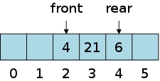
Now consider an array-based implementation similar to what we used for stacks. On the top right we show an array of capacity five into which we have enqueued -88, 2, 4, 21, 6 and then dequeued the first two items. We maintain two indices front, the index from which we will next dequeue and rear, the index into which we have just enqueued. Enqueuing x is accomplished by currentSize++; theArray[++rear]; and dequeuing is accomplished by currentSize--; return theArray[front++]
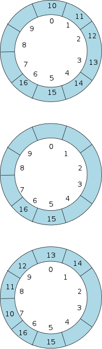
Now consider the billion item example above. Although currentSize()would never exceed 2, the capacity would grow to around a billion as we kept doubling the array because we first use slots 0 and 1, then 1 and 2, then 2 and 3, ... then 1111 and 1112, etc.
The solution is to use what is called a circular array
.
On the right we see an array of capacity 10 that we have drawn as a
circle.
But it is just an array.
We have done seven enqueues (10, 11, ..., 16), which leaves room for
three more items before filling the queue to capacity.
Now assume we do five dequeues (10, 11, 12, 13, 14), leaving only 15 and 16 enqueued (in slots 5 and 6 respectively). The result is the middle diagram.
On the one hand we still have only three slots available (7, 8, 9) because if we go beyond that we get to index 10, which exceeds the capacity and thus triggers an array doubling.
But this is silly, with only two slots used (5 and 6) we can see that 8 are empty. The bottom picture shows the result after requeuing 10, 11, 12, 13, and 14. The trick needed was not to use rear+1 but instead mod(rear+1,capacity).
Note that sometimes rear is smaller than front. For example in the bottom picture rear==1 and front==5. In the top two pictures currentSize==rear-front+1; in the bottom picture rear-front+1==-3, which can't be a capacity. But mod(-3,10)==7 which is indeed the correct value for currentSize. (Remember that % in Java is NOT mod, it is remainder.)
There are many. Indeed, we often speak of being queued up while waiting for a service.
For a British example, the line at a checkout or sporting event is called a queue in England.
Start Lecture #11
Remarks: Vote on midterm exam date.
Bug fixed in tuesday's code.
head/tail changed to front/rear.
Diagram enhanced.
Definitions: A nonempty tree is a collection of nodes, one of which is distinguished and called the root of the tree. The remaining nodes form zero or more nonempty trees called subtrees. There is a (directed) edge from the root of the tree to the root of each subtree. The node at the tail of an edge is called the parent and the node at the head is called the child. The common children of a single parent are called siblings.
More Definitions: The depth of a node is the length of the unique path to the root. The height of a node is the length of the longest path to a leaf. The height of a tree is the height of its root. The depth of a tree is the depth of its deepest leaf. The height and depth of any tree are equal.
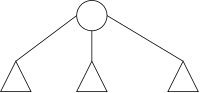
Trees are normally drawn with parents above children so we do not need to put arrows on the edges to show head and tail.
The diagram on the right shows a tree with the root having three subtrees. Each of these subtrees itself has a root and zero or more subtrees. Definitions like this are called recursive.
Homework: 4.1.
The root has depth 0; its children have depth 1; their children have depth 2; etc.
First Label all leaves with height 0. Then for any node all of whose children have been labeled, label this node with height one more that the maximum height of its children.
Homework: 4.2, 4.3.
Recall that for each linked class in chapter three, we needed two classes, a node class and a list class. The list class contained many methods and a few fields, including one or two that referenced a node (e.g., top, beginMarker, endMarker, front, rear) The Node class contained a few fields including the user data. A new list object would refer to a one or two node structure. As the list got larger more nodes would be added. But for any size list a node can references only a fixed number of other nodes (one other for single-linked lists; two others for double-linked lists).
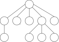
For a general tree, the situation is different. A parent can reference an arbitrary number of children. For the figure on the right some nodes have zero, one, three, or five children. Since the number of children is in principle unbounded and in practice can become large, we don't want to have fixed components in the node for each child (say child1, child2,, child3, etc).
For some important trees, called binary trees, there are never more than two children. In these cases the node would contain something like child1 and child2 components.
When a node can contain an arbitrary number of children, a natural implementation is to have a tree node reference a list containing the children something like
    class TreeNode<E> {
      E                      data;
      ArrayList<TreeNode<E>> childList;
    }
Instead, the list is normally built implicitly into the structure more like the following
    class TreeNode<E> {
      E           data;
      TreeNode<E> nextSibling;
      TreeNode<E> firstChild;
    }
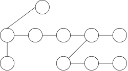
This gives rise to a picture on the right where the nulls at the end of each list are not shown nor are the nulls when there are no children. The horizontal lines go from left to right.
Note that this picture represents the same tree as the diagram above. The important difference is that each circle can have at most two edges leaving, which corresponds to each TreeNode having only two link fields (and one data field).
To traverse a tree means to move from node to node in a prescribed manner so that each node is reached (normally reached exactly once.
Definition: A tree node is called a leaf if it has no children. Occasionally non-leaves are referred to as interior nodes.
If you draw a tree the normal way (like the top diagram and not like first-child/next-sibling implementation), then the leaves are exactly the nodes that do not have any nodes below them.
All the traversals we will study visit the leaves from left to right along this bumpy bottom of the tree. The traversals differ in when the interior nodes are visited.
The terminology often used is that the traversal is the program that moves from node to node and, at some points, calls a user method normally named visit().
Consider the following two traversal algorithms, preorder() and postorder
preorder(node n) {                     postorder(node n) {
    visit(n);                              foreach child c left to right
    foreach child c left to right              postorder(c);
        preorder(c);                       visit(n);
}                                      }
The names are chosen to indicate when an interior node is visited with respect to its immediate children: In preorder() the interior node is visited pre, i.e., before, the children. In postorder() the interior node is visited post, i.e., after, the children.
Draw several trees on the board and do both traversals. Have visit() just print the data field.
// Use First Child / Next Sibling tree representation
public class DemoNextSib {
  private static class NSNode<E> {
    E         data;
    NSNode<E> nextSib;
    NSNode<E> firstChild;
    public NSNode(E data, NSNode<E> nextSib,
                          NSNode<E> firstChild) {
      this.data       = data;
      this.nextSib    = nextSib;
      this.firstChild = firstChild;
    }
  }
  private static void visit(NSNode node) {
    System.out.println(node.data);
  }
  private static void preorderTraverse(NSNode node) {
    visit(node);
    preTraverseChildren(node);
  }
  private static void preTraverseChildren(NSNode node) {
    NSNode n = node.firstChild;
    while (n != null) {
      preorderTraverse(n);
      n = n.nextSib;
    }
  }
  private static void postorderTraverse(NSNode node) {
    postTraverseChildren(node);
    visit(node);
  }
  private static void postTraverseChildren(NSNode node) {
    NSNode n = node.firstChild;
    while (n != null) {
      postorderTraverse(n);
      n = n.nextSib;
    }
  }
  public static void main(String[] arg) {
    NSNode<String> aaa=new NSNode<String>("AAA",null,null);
    NSNode<String> adc=new NSNode<String>("ADC",null,null);
    NSNode<String> ae =new NSNode<String>("AE", null,null);
    NSNode<String> adb=new NSNode<String>("ADB",adc, null);
    NSNode<String> ada=new NSNode<String>("ADA",adb, null);
    NSNode<String> ad =new NSNode<String>("AD", ae,  ada);
    NSNode<String> ac =new NSNode<String>("AC", ad, null);
    NSNode<String> ab =new NSNode<String>("AB", ac, null);
    NSNode<String> aa =new NSNode<String>("AA", ab, null);
    NSNode<String> a  =new NSNode<String>("A",  null,aa);
    preorderTraverse(a);
    System.out.println();
    postorderTraverse(a);
  }
}
The code on the right creates and traverses a tree implemented using the First-Child / Next-Sibling implementation.
It is perhaps surprising that there is no tree type, only a node type. All the tree would have would be a field root that referenced the node that was the root.
The node is a generic class with E representing the type of the data component. If you look at the main() method, you will see that the nodes created have Strings for data.
The visit() method is quite simple; it just prints the data component, which we have mentioned is simply a string.
The preorderTraverse() and postorderTraverse each have basically the same two lines; the primary difference is that their order is reversed.
It is in the preTraverseChildren and postTraverseChildren that we see really see the effect of the first-child/next-sibling implementation. Note that these two programs are basically identical.
The only interesting aspect of main() is the order in which the nodes are connected. The objective is to create a node only after its first child and its next sibling have been created. Thus, in particular leaves are created first. After that it proceeds right to left, bottom to top order. The result is the tree we have drawn (twice) above.
The string stored in the root is A. If a node has string x then its children have strings xA, xB, etc.
For convenience name of the variable used to reference a node is simply the lower case version of the string stored in the node. As a result I used 6 variables for the 6 nodes, which is more than necessary.
Sometimes you want the traverse() method to pass additional information to the visit() method, information that is not local to the node so visit() can't calculate the value by itself.
A common example is the depth of the node. The root is defined to have depth 0 and any child has depth one greater than its parent.
On the board extend the traversal example to pass the depth to visit and have visit indent the node's string with 2d blanks if the depth is d.
This gives the very beginnings of the tree listing produced by, for example, Windows Explorer.
Start Lecture #12
// Use First Child / Next Sibling tree representation
public class DemoNextSib {
  private static class NSNode<E> {
    E         data;
    NSNode<E> nextSib;
    NSNode<E> firstChild;
    public NSNode(E data,NSNode<E> nextSib,NSNode<E> firstChild) {
      this.data       = data;
      this.nextSib    = nextSib;
      this.firstChild = firstChild;
    }
  }
  private static void visit(NSNode node, int depth) {
    for (int i=0; i<depth; i++)
      System.out.print("      ");
    System.out.println(node.data);
  }
  private static void preorderTraverse(NSNode node, int depth) {
    visit(node, depth);
    preorderTraverseChildren(node, depth+1);
  }
  private static void preorderTraverseChildren(NSNode node,
                                               int depth) {
    NSNode n = node.firstChild;
    while (n != null) {
      preorderTraverse(n, depth);
      n = n.nextSib;
    }
  }
  private static void postorderTraverse(NSNode node, int depth) {
    postorderTraverseChildren(node, depth+1);
    visit(node, depth);
  }
  private static void postorderTraverseChildren(NSNode node,
                                                int depth) {
    NSNode n = node.firstChild;
    while (n != null) {
      postorderTraverse(n, depth);
      n = n.nextSib;
    }
  }
  public static void main(String[] arg) {
    NSNode<String> aaa=new NSNode<String>("AAA",null,null);
    NSNode<String> adc=new NSNode<String>("ADC",null,null);
    NSNode<String> ae =new NSNode<String>("AE", null,null);
    NSNode<String> adb=new NSNode<String>("ADB",adc, null);
    NSNode<String> ada=new NSNode<String>("ADA",adb, null);
    NSNode<String> ad =new NSNode<String>("AD", ae,  ada);
    NSNode<String> ac =new NSNode<String>("AC", ad, null);
    NSNode<String> ab =new NSNode<String>("AB", ac, null);
    NSNode<String> aa =new NSNode<String>("AA", ab, null);
    NSNode<String> a  =new NSNode<String>("A",  null,aa);
    System.out.printf("Preorder\n--------\n");
    preorderTraverse(a, 0);
    System.out.printf("\n\n\n\nPostorder\n---------\n");
    postorderTraverse(a, 0);
  }
}
Remark: I fixed the last program to produce the correct tree.
On the right is the above program enhanced to used the tree depth for indenting and to indicate which is preorder and which postorder. It produces the following output.
Preorder
--------
A
      AA
      AB
      AC
      AD
            ADA
            ADB
            ADC
      AE


Postorder
---------
      AA
      AB
      AC
            ADA
            ADB
            ADC
      AD
      AE
A
A binary tree is a tree in which no node has more than two children. So the tree in our previous diagram is not binary since one node has three children and another has 5 children.
class BN<T> {
  T     data;
  BN<T> left;
  BN<T> right;
  public BN(T data, BN<T> left, BN<T> right) {
    this.data  = data;
    this.left  = left;
    this.right = right;
  }
}
With such a small limit on the number of children, binary trees encourage neither having a list of children nor using the first-child/next-sibling representation. Instead, the structure on the right is used. The names left and right are nearly always used for the first and second child. Note that it is possible for left==null, but right!=null, and vice versa. The class on the right abbreviates BinaryNode as BN to save horizontal space.
As always, the bottom of the tree contains only leaves (nodes with no children). If very few nodes contain exactly one child then the tree gets quite wide and not very deep. In this case the depth is only O(log N) for an N-node tree. We shall see that, when organized properly, a binary tree form an excellent vehicle for storing data that needs to be searched frequently.
We have already seen preorder and postorder traversals. These can be used for arbitrary trees. Since binary trees nodes have at most two nodes, we can consider a traversal that visits the node between traversing the two children (traverse left, visit node, traverse right). This traversal turns out to be quite useful and is called inorder traversal.
When an inorder traversal is performed on a search tree (described
later) the values are printed in order
.
With this simpler node structure (all children referenced directly
from their parent), the traversals become a little simpler to code
and the relation between pre/post/in-order become quite clear.
Here is the Java implementation of each, where
again visit() is supplied by the user.
So that all three could fit horizontally on the screen, I needed to
abbreviate traversal
as trav
, BinaryNode
as BN
, and drop order
.
preTrav(BN<T> n) {           inTrav(BN<T> n) {           postTrav(BN<T> n) {
    visit(n);                    if (n.left != null)         if (n.left != null)
    if (n.left != null)              inTrav(n.left);             postTrav(n.left);
        preTrav(n.left);         visit(n);                   if (n.right != null)
    if (n.right != null)         if (n.right != null)            postTrav(n.right);
        preTrav(n.right);            inTrav(n.right);        visit(n);
}                            }                           }
Homework: 4.8.
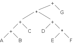
On the right we see an expression tree, commonly used in compilers. The leaves of the tree are values and the interior nodes are operators. The value of an interior node is the operator applied to the values of the two children. (If you want to support unary operators, such as unary minus, then those nodes have only one child.) So the tree on the right represents the expression (A+B+C)*(D+E*F)+G.
If you postorder traverse the tree with visit just printing the node's data, you get the postfix representation of the expression. Do this on the board. As we showed when studying stacks, it is easy to evaluate postfix using just a simple stack to hold the intermediate results.
inorderTraverse(BinaryNode<T> n) {
  if (n.left != null) {
    System.out.print('(');
    inorderTraverse(n.left);
    System.out.print(')');
  }
  visit(n);
  if (n.right != null) {
    System.out.print('(');
    inorderTraverse(n.right);
    System.out.print(')');
  }
If you preorder traverse the tree, you get the prefix representation. Do this on the board as well.
What about inorder? It doesn't work because our ordinary (infix) notation requires parentheses.
The fix is easy, just add the parens explicitly as part of the traversal. It would be harder to only put in the essential parentheses. The resulting method is shown on the right. On the board apply the method to the tree above.
We now give the simple algorithm for converting a postfix expression into an expression tree. To emphasize its similarity to the algorithm (see section 3.6.3) for evaluating postfix expressions, we show them side by side below.
Scanner getInput = new ...;
while (getInput.hasNext()) {
    token = getInput.next();
    if (token is an operand)
        stk.push(token);
    else { // token is operator
        tmp = stk.pop();
        stk.push(stk.pop() token tmp);
    }
print stk.pop();
    Scanner getInput = new ...;
    while (getInput.hasNext()) {
        token = getInput.next();
        if (token is an operand)
            stk.push(BN(token,null,null));
        else { // token is operator
            tmp = stk.pop();
            stk.push(BN(token, stk.pop(), tmp);
        }
    print stk.pop();
On the board start with the postfix obtained from the expression tree above, apply the method, and see that the tree reappears.
To start lets take a special case. Assume the data items are Longs and that no two data are equal. Then imagine a binary tree with one item (Long) in each node having the property that, for any node
Draw one of these trees on the board and show how a
divide and conquer
approach can be used to search for any
item without ever having to go back up the tree.
If the tree has very few nodes with one child, then its hight is small (O(log N)) and the search is very fast.
Start with an empty tree (no nodes), pick numbers at random, and insert them in the right spot (without moving any existing nodes).
Homework: 4.9
Start Lecture #13
Remark: Hand out the code.
I apologize in advance for how complicated this looks. In fact, Java generics are quite tricky and complicated. You might want to read the first few pages of the brief tutorial on the home page. If you are brave, very brave, you can try the FAQ also referenced on the home page.
Enough stalling. The header line is.
public class BinarySearchTree<E extends Comparable<? super E>>
Oh, my gosh.
A binary search tree (BST for short) is a binary tree that we will use for searching. Like any binary tree, it has three fields, left, right, and data. The first two reference the left and right subtrees as expected. The third is the user's data that we are storing and that we will wish to search for.
public class BST<E extends Comparable> {
  private static class BSTNode<E> {
    E          data;
    BSTNode<E> left;
    BSTNode<E> right;
  }
}
Since we shall use a divide and conquer approach, where we check to see if the current data (datum in English) is less than, equal to, or greater than, the item we are searching for, we need the type of data to support comparisons. In java-speak we need its class to implement Comparable (between <> we write extends not implements). So we will want to support BST<Long> and BST<String>, but not BST<Integer[]>.
So what is wrong with the code on the above right?
Not much, but the scary one above is better.
If we used the above version we would get an
unsafe or unchecked operations
warning from the compiler.
In general the Java generics are imposing, but do have the huge
advantage that they convert a bunch of run-time errors (those that
might occur when there are unsafe or unchecked operations
into compile-time errors.
The scary header uses the generic Comparable<>
instead of the pre-generic form Comparable.
public class BST<E extends Comparable<E>> {
Ok, but what is the ? super
business.
That is, why can't we just replace the header line on the top right
with the one on the immediate right?
This is a consequence of the somewhat delicate Java rules for generics and inheritance. We will describe it later.
The only data field is root, a BSTNode that (naturally) references the root of the tree. The only constructor sets this node to null, representing an empty tree.
As mentioned this class has three fields data,
left, and right.
The primary constructor simply takes in values for the three fields
and performs the standard assignments this.x=x;
.
Since many new nodes are leaves, we define another constructor with just data as a parameter. This constructor calls the primary constructor giving null for both left and right.
There are no public methods; users do not deal with nodes.
These are trivial: an empty tree is one whose root is null.
We do 4.3.2 before 4.3.1 since finding the max and min is easier than general searching. Indeed, for the min we just keep going left and for the max we just keep going right. When we can't go any further, we have found the min or max. Show this on the board for
Note that the public versions return just the data, of type E; whereas the private version returns a node. The node will prove useful in remove().
Homework: Rewrite
findMin and findMax using while
instead of for
loops.
This is a more serious routine that shows the basic recursive structure of a binary search tree. The public method has just one parameter, the data value to search for and returns a boolean indicating whether this datum is present in the tree.
The helper (private) method accepts a second parameter giving the node in the tree where to begin the search. Initially, this is the root, but moves down the tree as the searched proceeds.
The helper initially checks if the node is null, which indicates that the value does not exist in the tree. The helper then compares the searched-for value with the data at the current node. The outcome of this comparison determines the next action. If the two are equal, the searched-for value has been found and true is returned. If the search-for value is less, the search moves to the left subtree (all values in the right subtree are greater than the value at the current node so cannot possibly match). Similarly, if the search-for value is greater, the search moves to the right subtree.
Draw pictures showing the steps for several trees, including empty and one-node trees.
Inserting a value is actually quite similar to searching for that value. Conceptually, to insert you first search and proceed based on the search outcome. If the value is found, the insert is done (alternatively you could bump some counter). If the value is not present, the search will end at a null node that becomes the new node containing the value.
Note how the code passes the revised subtree back up to the various recursive helper calls to the original public insert method. In fact, only one node changes, the parent of the new node. Higher in the tree, we are replacing left or right with the identical reference.
Once again draw some pictures on the board.
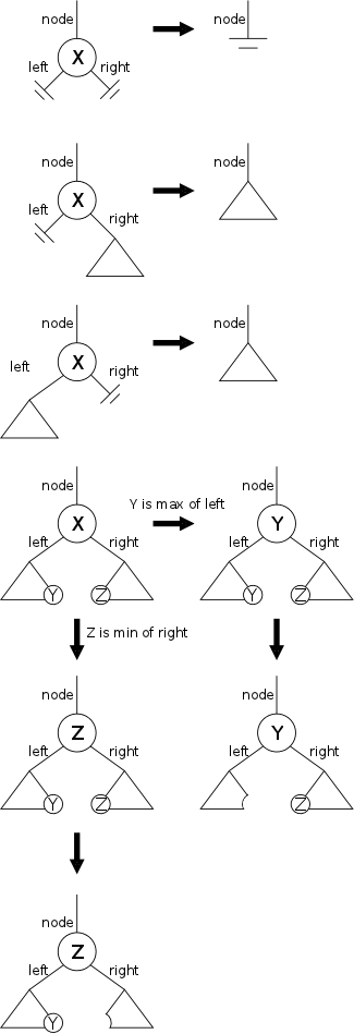
This is the trickiest method of the bunch. Like inserting, removing is searching plus. What makes it tricker than inserting is that we always insert a leaf, but we may be removing an interior node and thus need to restructure the tree.
Remove moves down the tree the same as for searching or inserting. If null is reached, the data value is not present and we are done. The interesting case is when we do find a node with the datum in question and now the fun begins. Call that datum X.
If this node is a leaf, it is easy; just set the node reference to null as shown on the top right. The line labeled node is vertical indicating that this node can be either a left or right child of its parent, or can be the root of the tree.
In the remaining frames of the diagram a triangle represents a non-empty subtree, i.e., the corresponding reference is not null.
In the second frame, the node has a left child only. Then we replace the node with its left child (in Java-speak node=node.left;. This works because: (1) any subtree of a binary search tree is itself a binary search tree, and (2) if the node X was a right child of its parent (i.e, its value was greater than its parent's) then either subtree of X is also greater that the X's parent (similarly, if X was a left child).
In a like manner, if the node has a right child only, we replace the node with its right child (node=node.right;), as shown in the third frame.
The fourth frame, depicting the case where the node has both a left and right child is the star of the show. We need to replace the value X by one that is still less than everything to the right and greater than everything to the left. We have exactly two choices.
We can pick Y, the maximum of the left tree, which is the largest value smaller than X, i.e, Y comes right before X in a sorted listing of the elements. Alternatively we can pick Z, the minimum of the right subtree, which is the value coming right after X in a sorted listing.
Note that although it is the value X that is removed, the deleted node is the one that held either Y or Z.
Care is needed in propagating the result back up the tree. Changing node itself has no permanent effect due to call-by-value semantics. However, changing node, returning node, and then having the caller set node.left or node.right to the returned value does have an effect due to reference semantics. This is the same reason that when an array is passed and the callee changes an element of the array, the caller sees the change.
Start Lecture #14
Midterm Exam
Start Lecture #15
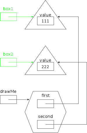
The median grade on the midterm was 88.
The diagram on the right is the answer to question 3. The part is green is optional.
The code below is an answer to question 5. Only reverseList() is required. Most of the rest is to test it.
public class LinkedList {
    private int  theSize = 0;  // initially LinkedList is empty
    private Node beginMarker;
    private Node endMarker;
    LinkedList () {
	beginMarker = new Node(0, null,        null);
	endMarker   = new Node(0, beginMarker, null);
	beginMarker.next = endMarker;
    }

    private static class Node {
	private int  data;
	private Node prev;
	private Node next;
	Node(int data, Node prev, Node next) {
	    this.data=data; this.prev=prev; this.next=next; }
	Node(int data) { this(data, null, null); }
    }

    private void printList() {
	System.out.println("Forward");
	for (Node node=this.beginMarker.next; node!=endMarker; node=node.next)
	    System.out.println(node.data);
	System.out.println("Backward");
	for (Node node=this.endMarker.prev; node!=beginMarker; node=node.prev)
	    System.out.println(node.data);
    }

    private Node addBefore(Node node, int i) {
	Node newNode = new Node(i, node.prev, node);
	node.prev.next = newNode;
	node.prev = newNode;
	theSize++;
	return newNode;
    }

    private static void reverseList(LinkedList list) {
	// remove the first node from beginMarker (using next)
	// reinsert it as the last node from endMarker (using prev)
	Node lastInserted = list.endMarker;
	Node node = list.beginMarker.next;
	while (node != list.endMarker) {
	    Node nextNode = node.next; // save for next iteration
	    node.next = lastInserted;
	    lastInserted.prev = node;
	    lastInserted = node;
	    node = nextNode;
	}
	list.beginMarker.next = lastInserted;
	lastInserted.prev = list.beginMarker;
    }

    public static void main(String[]arg) {
	LinkedList list = new LinkedList();
	Node one   = list.addBefore(list.endMarker, 1);
	Node two   = list.addBefore(list.endMarker, 2);
	Node three = list.addBefore(list.endMarker, 3);
	list.printList();
	reverseList(list);
	list.printList();
    }
}
Often instead of actually removing a deleted node, we employ so
called lazy deletion
and just mark the node as deleted.
This shortens deletion time at the expense of a larger resulting
tree.
Lazy deletion is popular if the number of deletions is expected to
be small.
We will see this issue again soon when we study AVL trees.
We use a standard inorder traversal. Unlike our previous version, instead of checking if left and right are null, we always descend and then check if the node we arrive at is null. This is very slightly less efficient and very slightly shorter.
Rather than print nothing for an empty tree, the public method checks for null and prints a message.
Homework: Modify printTree() to indent proportional to the depth.
These classes are pretty silly, but I do believe they illustrate two points very well: the value of toString() and the necessity of the scary header.
The class TwoIntegers, as the name suggests, has two data fields, both Integers. It has the standard constructor.
The derived class ThreeIntegers has three data fields. Its constructor uses the above constructor for the first two fields and itself sets the third, new, field.
Each class overrides the toString() method defined in the Object class. TwoIntegers.toString() produces an order pair in the mathematically standard notation; ThreeIntegers produces the equivalent order triple. This usage eases printing out the tree in an informative manner.
TwoIntegers defines an ordering of its members based on the sum of the two values. This is a weak ordering since many pairs of Integers have the same sum, but it is enough to define compareTo() and thus the class TwoIntegers implements Comparable<TwoIntegers>.
Since ThreeIntegers extends TwoIntegers it also implements Comparable<TwoIntegers>, but it does not have its own compareTo() and hence does not implement Comparable<ThreeIntegers>.
We already understand that the data field needs some sort of Comparable so that we can decide if one element is greater equal or less than another.
We also understand that just plain Comparable gives up the compile-time-error-checking of Java generics.
public class BST <E extends Comparable<E>>
public class BST <E extends Comparable<? super E>>
What remains to understand is why isn't the top line on the right good enough. Why must we use the horror below it? For a start what does the bottom line mean?
The ? is a wild card that, when used alone, matches any type so T extends Comparable<?> would be satisfied by any type T that implements Comparable<X> for some type X. That is elements of T can be compared to something, not especially useful.
The bounded wild card
? super E matches any type
T that is a supertype of E.
In other words it matches any type T from which E
is derived (i.e, a type T of which E is a subtype).
From this we can see that the horror is needed. Specifically, BST.java would not compile with the simpler version above it!
Why?
In main() we see a declaration using BST<Threeintegers>. If we used the simpler version we would need that ThreeIntegers could be plugged in for E, i.e., that
ThreeIntegers extends Comparable<ThreeIntegers>
But the last paragraph of 4.3.F notes that ThreeIntegers
does not
implement Comparable<ThreeIntegers>; so the
compilation would fail.
On the other hand the horror just requires that E implements Comparable<T> for T some superclass of E. This IS satisfied since ThreeIntegers implements Comparable<TwoIntegers> and TwoIntegers is a superclass of ThreeIntegers.
Question: Given a tree with N nodes, what is the longest time that can be required for an insert or a delete?
The worst case occurs when the tree is a line, i.e., no node has more than one child. In this case starting at the node, we need to descend N-1 times to get to the leaf and this could be the insertion or deletion site. Since descending takes a constant number of instructions, the total time is O(N). (It would be better to say Θ(N), but we will be sloppy and use only O()s.)
One can show that, under the assumption that all possible insertions are equally likely, most trees are not very high. Indeed, the average height for an N-node tree is O(log(N)).
The goal of AVL trees (the name comes from the initials of the three discoverers) is to reduce the worst case time to the average case time for all operations. Specifically, searching, inserting, and deleting are to have logarithmic complexity, (i.e., all run in time O(log(N)) for a tree with N nodes. This is accomplished by ensuring that the height of all AVL trees is O(log(N)).
We shall see that AVL trees (and heaps, later in the semester) require both structure and order properties. The order (or perhaps ordering) property is that of any binary search tree: The key of the left child is less than the key of the parent, which in turn is less than the key of the right child.
Thus the order property constrains what elements can appear where in the tree. The structure property in contrast constrains what shape trees are permitted. As we shall see AVL trees are required to be height balanced in a sense to be made precise right now.
Recall that the height of a leaf is 0 and the height of a non leaf is the 1 plus the maximum height of its children. Draw some pictures.
The key idea is that we keep the tree height balanced
, that
is it is about the same distance from a given node any leaf in the
subtree under this node.
Specifically:
Definition: An AVL tree is a binary search tree having the property that at any node the right and left subtrees have heights that differ by at most one. (The height of an empty tree is defined to be -1.) This requirement that the heights differ by at most 1 is called the balance condition.
We can see that any tree with fewer than 3 nodes is AVL. Draw some pictures to show this.
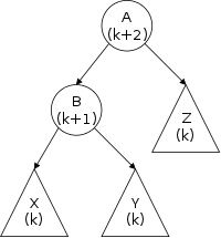
Since tiny trees are AVL the only way a tree can become AVL is via
an insertion or a deletion.
We employ lazy deletion
so that a delete operation does not
change the tree shape and hence the balance is also unchanged.
The real work is to enhance the insert routine so that, if tree to
goes out of balance, the balance is restored via
a rotation
.
Assume we have a AVL and try to insert an item. Often the tree remains AVL, but not always; the item we add may throw a node out of balance. That is the node's left subtree becomes 2 higher (or 2 lower) than its right subtree.
The top diagram on the right shows a typical setup that is in balance but can become out of balance if a node is added to either the x or y subtree at a point that makes the subtree one level higher (i.e., the height increases from k to k+1. In either case B will become height k+2, which makes A out of balance since its children have heights differing by 2.
Remember than any insert adds a leaf to the tree and note that the only heights that can be affected are on the path from the inserted leaf up to and including the root of the tree. Hence these are the only nodes that can become out of balance. Assume in the picture that A is the lowest node to go out of balance.
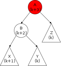
Although it might appear that having a leaf added to x or added to y would be the same, this is not the case. We will first do the easier case of the leaf being added to x and do the harder case with y later. The difference is that the first situation has a node added to the left subtree of the left child of A; whereas, the second has a node added to the right subtree of the left child. It is the asymmetry that makes it (a little) harder.
The resulting situation is shown in the second diagram on the
right; the node A is in red to indicate that it is the
(lowest) node out of balance.
The insertion to the tree occurred below A and all the
changes to the tree will occur in the subtree rooted at A.
We will see that the fixed
subtree (now rooted at B)
has the same height as the ORIGINAL subtree rooted
at A.
Thus all the nodes above this subtree will have their
original height and thus will remain in balance.
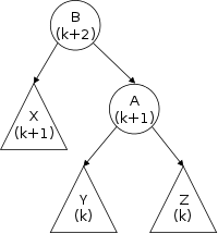
The fix is to rotate
the tree to get the next diagram.
You need to check that the rotation is legal
.
That is, do we still have a binary search tree and is it in
balance.
The answer to both questions is yes!
But we just looked at the lowest node out of balance.
Time to go up the tree and fix the rest.
Not necessary.
Note that the top of the resulting diagram has a root that is the
same height as the original diagram.
Therefore the nodes above this tree have their original heights and
everything is back in balance.
The symmetrical case where a node is added to the right subtree of
the right child of the lowest out of balance node, is handled
symmetrically.
In both of these cases, the node is added to an outside
subtree; what remains is to consider adding a node to an
inside
subtree.
Specifically, we will return to the original
diagram, and assume a node is added to the y subtree in a
way that raises its height to k+1.
Start Lecture #16
But before moving on to this so-called double-rotation
, let
us follow the book and practice single-rotations by starting with an
empty tree and adding nodes with data values 3, 2, 1, 4, 5, 6, 7 in
that order.
Remark: The traversal in printTree is indeed a little shorter. It contains one if instead of two. On the board last time I wrote it differently and added a line.
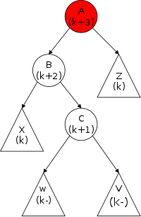
Recall that we now are considering the case where we add a node to an inside subtree. Let's do the case where the insertion raises the height of the right subtree of the left child of the lowest height node to go out of balance. (A symmetric solution works if the loss of balance is due to raising the height of the left subtree of the right child.) Specifically, we return to the original diagram and add a node to the y subtree in a way that raises its height to k+1.
As mentioned above, this case is a little more involved than the single-rotation we did previously. The augmented y subtree is definitely not empty since we just added a node to it. Call the root C and call its subtrees w and v.
These two subtrees must be of height k or k-1 (in
fact one must be k and the other k-1).
In the diagram I show the heights as k-.
This is an abbreviation for k or k-1
.
As with single rotation, the solution is to move the nodes around and reconnect the subtrees. The solution is shown in the bottom diagram on the right.
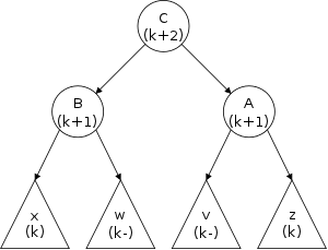
Note that, as with single rotations above, the subtrees rearranged in double rotation must remain in the same right-to-left order as they were originally in order to maintain the order property of binary search trees, which states that data in the left subtree is less than the data in the parent, which is in turn less than the data in the right subtree.
We must again check that the nodes A, B, and C remain ordered correctly and again they do.
Let's again follow the book and continue our example by now inserting 16, 15, 14, 13, 12, 11, 10, 8, and 9 in that order.
Homework: 4.19.
Remark: I added some homework problems to this entire chapter. They are not assigned this year, but might well prove worthwhile to look at when studying for the final.
As mentioned previously an inorder traversal can be used to list the data elements in sorted order. Thus given N data items, you can insert them one at a time into an initially BST and then do an inorder traversal to effect a sort of the items.
Since each insertion and removal requires (log(N)) the total time to sort all N items is O(N×log(N)), which we shall see later is very good.
Recall that to calculate the height of a node, you need the heights of its children. Thus an inorder traversal is perfect; the visit() operation labels the current node with its height using the (already calculated) heights of the children.
Note that this works for any tree, not just binary trees.
Recalling that a node's depth simply one plus the depth of its parent, we see that a preorder traversal works perfectly. The visit() method calculates the depth of the node using the (already calculated) depth of its parent.
Again, this works for any tree, not just binary trees.
Occasionally you wish to visit the nodes in a breath-first, not depth-first, order. That is first visit the tree root, then all nodes of depth 1, then all nodes of depth 2, etc.
Rather then a recursive traversal program (for which Java supplies a stack to hold values of active invocations), a non-recursive, queue-based program is used.
I don't believe we will use breath-first traversals.
Start Lecture #17
AVL trees work very well (O(log(N)) indeed, but we have been making two tacit assumptions.
number.
E  data;
E  key;    // comparable
T  record; // entire entry
As mentioned often only a portion of the data item is searched for. This is easy to incorporate in our program. All we need do is to replace the top line on the right with the two below it. Then we do the searching using the key and when it is found, we retrieve the entire record (or insert a new node with both the key and the record).
When the database is too large to fit in memory, we need to store some/most/all of it on disk.
Lets begin with an easy case where an AVL tree with just the keys would fit in memory. It is the very large records that cause the problem. Then we can leave the AVL tree, with (key,record) pairs, essentially in tact. We just have the record field refer to a location on disk.
Note that only one disk access is needed per retrieval or insertion, the minimum possible if the true record is to be stored on disk.
Now lets assume that either the keys are very big (not likely) or there are just so many of them (the normal case) that we can't even fit a tree of just the keys in memory.
We first try the simple (simple-minded?) idea of putting the entire AVL tree on disk. In memory we keep just the disk address of the root node. That node contains all the data for the root (key and record) as well as the disk address of the left and right children.
From an asymptotic analysis point of view, nothing has changed: Each insert or retrieval, requires O(log(N)) steps each needing just a constant number of operations (1 disk access, plus a few dozen machine instructions). So we have the same complexity as before.
But from a pragmatic point of view, the solution
has changed
from excellent to awful.
That one disk access corresponds to a dozen or so
million machine instructions.
While this is still a constant, it is a large one indeed.
I don't believe anyone uses this solution.
The problem is that O(log(N)) is too big. If N=107, which is not uncommon, then log(N) = log2(N) is about 24. We want to replace this by say log128(N), which would be about 4.
To reduce the number of steps from log2(N) to log128(N) requires that the depth of the tree be similarly reduced, which in turn requires that, instead of a binary tree, we use a 128-ary (binary, tertiary, quaternary, etc) tree.
For a binary tree, we kept one key in the node and used it to choose the left or right child. Now we would need to keep 127 keys to choose between the 128 children, and that is the main idea of B-trees.
My choice of 128 was arbitrary, the real answer (the bigger, the better) depends on the size of the key. Assume that a single disk access retrieves 8KB = 8196 bytes (this is typical). Assume a key is 54B and 8B are needed to specify a disk block. For the node to have M children, we need to specify M disk blocks and this needs M-1 keys. So for our example the space required would be 8M+54(M-1) bytes. We want a node to fit in a single block so we need 8M+54(M-1)<8196. The largest M satisfying this inequality is 133 and we will have a 133-ary tree.
But just as a binary tree has some nodes with fewer than 2 children, our tree will have a maximum of 133 children at any node. Some nodes will have fewer children.
Assume the full data item (key+record) is 700B. Normally, the record includes the key so there is no sum. In what follows we store just the record. Thus our 8196B disk block can hold L=11 700B records.
Now lets drop the numbers and just say that 1 node (which equals 1 disk block) is big enough to contain either
Then a B-tree of order M is an M-ary tree with the following properties. (Actually, there are several variants of B-trees including B*-trees and B+-trees. I believe that what follows is closest to a B+-tree)
The key point is that (except for the root) all non leaves have many children (at least ⌈M/2⌉) and hence the tree is not very high. This means that not many disk accesses are needed to find a record.
To make our example manageable, let us make an unreasonable choice of parameters and set L=3 and M=4. Perhaps even more unreasonably assume that the record is just the key.
On the board, start with an empty B-Tree and add (in this order) items with the following keys: 10, 50, 40, 30, 31, 32, 33, 34, 35, and 36.
Initially, the tree is empty. The first insert creates a leaf holding the one record, but having room for two more. This leaf is the root of the tree (it is the entire tree). After 2 more inserts, the root is filled with L=3 records (the top frame on the right).
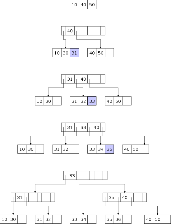
Adding a fourth record (50) causes the root to split into two leaves with a non-leaf root added. This is the second frame without the blue 31 record. To save space the middle three frames each represent two time points, one before the blue record is inserted and one after. Note that the key (40) placed in the root is the smallest key found in the subtree referenced by the child pointer in the root to the right of the 40.
The root currently has two children; it can have up to M=4 children and hence can hold up to M-1=3 keys. A fifth record is added with no splitting required, which gives the entire second frame as drawn, i.e., including the blue 31.
At this point the left leaf is full and splits when the sixth record (32) is added. Since that record has key less than 40, it must go to the currently full left leaf. This is the third frame without the blue 33.
The seventh record (33) is then added with no splits needed, giving the entire third frame as drawn.
At this point the middle leaf is full and splits when the eighth record (34) is added (to this leaf). The result is the fourth frame without the blue 35.
The ninth record is added with no splits, giving the fourth frame as drawn. Now the third leaf is full.
At this exciting moment the tenth record (36) is added. It goes to the full third leaf causing it to split, producing a total of five leaves. But the root can only have four children so it must split. The five children must be divided between the two non-leaves: one will have 2 children, the other 3. I chose to let the left non-leaf have 2 and the right have 3. We now need a new root, which is added. This gives the fifth frame and completes the insertions. Note that the key in the root (33) is the smallest key in the subtree referenced on the right not the small key in the child referenced on the right.
The item will be at a leaf and is removed. The question is what to do if the leaf now has below the minimum number of items (⌈L/2⌉).
First we try to take an item from a neighboring sibling (adjusting the corresponding key in the parent. This is not possible if all such neighbors themselves have the minimum number of items.
If this first attempt fails, we combine the node with one of the neighboring siblings, reducing the number of children in the parent by 1. If the parent, now has below the minimum number of children (⌈M/2⌉), then the parent tries to obtain one from one of its neighboring children. If the parent cannot get to the minimum, it combines with a neighboring sibling and the procedure repeats.
If we get to the root and it falls below the root minimum
,
which is 2, then we have a root with just one child.
We can remove this root and make the one child the new root.
Finally, if we remove the last item, we get an empty tree.
On the board remove all the items from the tree constructed in the last section. This tree is repeated on the right for clarity.
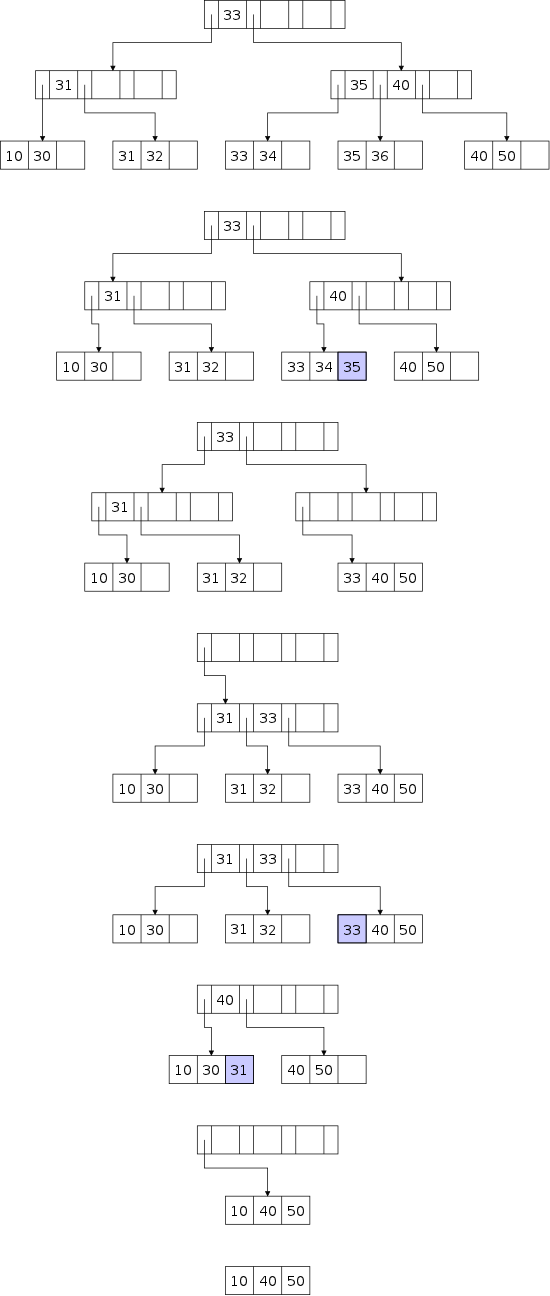
When we delete 36 from the top frame on the right (which is the final frame of the insert diagram), we leave a leaf with only one record (35), which is below the legal minimum of ⌈L/2⌉=2 records. Since both sibling neighbors are at their minimum, we cannot take a record from them. Hence we must merge the singleton leaf with one of the sibling neighbors. I chose to use the left neighbor. The result is the second frame, including the blue record.
Note carefully that, although we now have the same four leaves that we had in the penultimate frame for the insertion, we do have the same tree. Now the four leaves have two parents and the root above that. Previously, the four leaves just had one parent, the root. The reason the ambiguity occurs is that a non-leaf can have from ⌈M/2⌉=2 to M=4 children so four total children can have either one or two parents. The general point is that a B-tree is not determined simply by its leaves.
Deleting the next record (35) simply removes the blue 35. Subsequently removing 34 is probably the most complicated possibility so I will show several steps.
With the 34 gone, the resulting leaf has just the 33 record, which is below the minimum. Since the only sibling neighbor is at its minimum, no record can be taken from it. Hence we merge the singleton leaf with its (only) sibling neighbor, resulting in the third frame on the right.
But now the rightmost non-leaf has only one child, which is below the minimum of ⌈M/2⌉=2 children. Since its only sibling neighbor has the minimum number of children, none can be taken. Hence these two nodes must merge, resulting in the fourth frame.
But now the root has only 1 child, which is below the root minimum of 2. The result is that the root is deleted and its only child becomes the new root, shown in the fifth frame, including the blue 33.
Deleting the 33 record just removes the blue 33 AND changes the second key in the root from 33 to 40.
Deleting the 32 results in 31 being a singleton leaf. Since its sibling neighbors are at their minimum, a merge is required. I choose to merge with the left sibling resulting in the 6th frame, including the blue 31.
Deleting 31 simply removes the blue record.
Removing 30 again leaves a singleton leaf that must be merged with its only sibling, first resulting in the 7th frame. Since the root has only one child it is removed resulting in the final frame.
The final three records are removed with no extra operation except for removing the root when the tree becomes empty.
Homework: Start with the example produced in the preceding section and perform the following operations in the order given.
Read.
Here is an easy/fast way for NYU to store and access data about all of us. I checked and my NYU id is N13049592, which has 8 digits (let's ignore the initial N). So simply declare an array of items with indices from 00,000,000 to 99,999,999. My record is stored in slot 13,049,592. Simple.
Of course the trouble is that we are declaring an array of size 100,000,000 and will use well under 100,000 of these entries. So 99.99% of the entries are wasted. No good.
So we need a function h(x) (called a hash function) such that, for x in the range 0-99,999,999, h(x) is in the range 0-99,000. Then we store a record with key x in array slot h(x). Finding such a function is easy! For example h1(x)=x/1000 would do the job and would store my record in array slot 13,049. Even easier would be h2(x)=42 which stores my record in slot 42.
Of course h2 is awful as it would store all records in slot 42. Indeed, h1 is not great either since it would store any record with key beginning 13,049 in slot 13,049.
So in summary everything is except for three issues.
Nin my net id)?
The first issue is not hard. Using ascii or UTF8, or Unicode, arbitrary characters can be assigned numerical values and an arbitrary String becomes a very, very long. The remaining two issues are more substantial, especially the second, and are dealt with next.
Start Lecture #18
Choosing a good hash function is not trivial and choosing an excellent one is hard unless you know something about the keys that will be encountered.
public static int hash (String key, int tableSize) {
  int hashVal = 0;
  for (int i=0; i<key.length(); i++)
    hashVal = 37*hashVal + key.charAt(i);
  hashVal %= tableSize;
  if (hashVal < 0)   // % is NOT mod
    hashVal += tableSize;
  return hashVal
We will not pursue this issue in any depth and will be content to use the Java program on the right, which hashes an arbitrary string so that it fits in an array (often called a table) of size tableSize. Note that tableSize is normally chosen to be a prime number.
The loop computes a polynomial using Horner's rule. Early characters in the string are multiplied by higher powers of 37. Why 37? Because it works well :-).
The polynomial computation might well overflow and produce a negative value. Since % in Java is NOT mod, but instead remainder; the result of % can still be negative, which explains the final if statement.
This concludes our skimpy treatment of the hash function. The only issue remaining is how to deal with collisions.
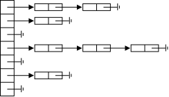
With separate chaining, collisions are handled by employing a list for all items that hash to the same value. The diagram on the right illustrates the data structure using linked lists.
In this example one would first choose a hash function that generates an integer (for example the method hash() above) and then take the result mod 7. This procedure selects a slot in the array.
For a retrieval, insert, or delete, the item is hashed to find the corresponding linked list and then the search, insert, or delete is performed there. As usual, one needs a policy for inserting an already present item or deleting an item that is not present.
Recall that for binary search trees, we needed the data objects to be members of a class that implemented some form of Comparable. This was because we needed to know if one object was less than, equal to, or greater than another, to decide whether to go left, declare success, or go right.
public class Equal {
  public static void main(String[] arg) {
  class Nothing {
    int x;
    Nothing(int x) { this.x = x; }
  }
  Nothing n1 = new Nothing(8), n2 = new Nothing(8);
  System.out.println("n1.x="+n1.x+" n2.x="+n2.x+
  		   ", but n1=n2 is " + n1.equals(n2));
  }
}
n1.x=8 n2.x=8, but n1=n2 is false
Now we just need to know if two objects are equal; the code in the book uses the equals() method of the class. Note that this is probably not the equals() method inherited from the class Object since that method returns true only if the two operands are the same object.
For example, the code in the top frame produces the output in the bottom. Although the value of the two instances of Nothing are equal, the instances are not.
To make the equals() method useful for comparing values, we would need to define our own, that compared the corresponding x components. Recall that I did this for the class TwoIntegers.
In fact you don't have to use a linked list as shown in the diagram, but it is common to do so. You could use something fancy like a binary search tree, even an AVL tree (in which case equals() would not be enough).
Before we compare objects for equality with other objects on their list, we need to hash them to the correct list to begin with. Typically the object, or at least the key, is a string and we use the hashCode() method from the standard library to produce an int and then take this result mod tableSize (again remembering that % in Java is NOT mod).
In principle the array can be tiny, even size 1, but that would be a poor choice. The result would be that many objects (all objects for size 1) would hash to the same list and the list search could be lengthly.
For a general-purpose hash table the ideal array size depends on
the application so an adaptive approach is normally use.
The array is created to be of modest size and if the number of items
becomes too large
, the size is doubled.
A common interpretation for too large
is that the number of
item in the hash table is larger than the number of lists.
See section 5.5 for more information on the enlarging process, which
is called rehashing.
There is another popular method for handling collisions that is
rather different from separate chaining.
In these so called probing
methods the only data structure is
an array of items, no pointers are used.
The procedure starts the same: the object is hashed to an index of the array. If this slot is full and contains a different object, then a new slot is chosen and the process is repeated. There are several popular choices for which new slot to choose, we will only look at the simplest one, which is called linear probing.
One point needs to be raised before discussing which alternative slot to choose. With separate chaining, the array is typically chosen to have the same size as the total number of items stored (remember that several can be stored using one slot). With probing the table is chosen to be significantly larger than the number of items stored.
The so called load factor, λ = numberOfItems / numberOfSlots, is typically around 0.5.
This scheme is easy to describe: if the current slot has something else in it, use the next slot.
Example. Assume you are want to insert x and hash(x)=35, you check slot 35.
Searching is similar, if you find x, you have succeeded; if you encounter an empty slot, x is not present; if you find another value try the next slot.
Why is this called linear probing? Certainly the hash() function is not linear. The reason is that the ith probe looks in location hash(x)+i and the function f(i)=i is linear. Indeed the scheme would be called linear probing if you used hash(x)+f(i) for any linear function, but we will just use the simplest f(i)=i.
Homework: 5.1a, 5.1b
Use hash(x)+f(i) where f(i) is quadratic. For example hash(x)+i2.
Use hash(x)+i*hash'(x) for some second hash function hash'(x).
For rehashing there are three questions to decide.
The decision to rehash is normally based on the load factor λ.
Normally, the new array size is double the old size.
After the new array is created, each element on the old hash table is rehashed (hence the name) using the new tableSize and inserted into the new hash table (directly in the array for probing and on a list for separate chaining).
Homework: 5.2.
Read.
Start Lecture #19
The basic idea of a priority queue (I would prefer priority list since the structure is not FIFO, but priority queue is standard) is to support efficiently two operations: insert and deleteMin. Note that not part of the model is deleteFirstInserted.
There are trivial, but poor implementations. You could just use any old list (say an array). Then insert is fast (if an array, you would insert at the high end). Indeed it is O(1). However, deleteMin is slow O(N).
You could use an array but insert in sorted order. Then deleteMin is fast O(1), but insert is slow O(N).
You could use a binary search tree, then the average case is fast O(log(N)) for both operations (not obvious since the deleteMin is not a random delete), but the worst case is slow O(N).
You could use an AVL tree, which is not bad. Both insert and deleteMin are fast O(log(N)) in worst case. The constants are somewhat large and there is space used for the pointers.
Our main data structure for this chapter, the binary heap, will match the complexity of AVL but not use pointers. It will instead be array based.
Note that a heap cannot find an arbitrary element in O(log(N)) time. It is a more specialized data structure than an AVL tree, which can do essentially anything (e.g., retrieve, insert, delete, find min, find max) in O(log(N)) time. Thus it is not so surprising that a heap can be simpler (array-based) than an AVL tree.
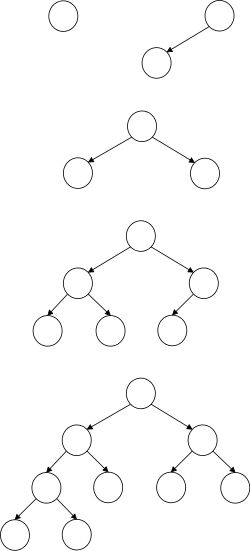
Really there are many kinds of heaps, but we will concentrate on
just this one, which is the most common.
Indeed when one says a heap
, the generally mean a binary
heap.
Like an AVL tree a heap has both a structure and order property. Also like an AVL tree, the heaps properties can be destroyed by standard operations and thus these operations must be extended with code to restore the properties.
The structure property is fairly simple: a binary heap is a complete binary tree, that is every level is filled except possible the lowest, which is filled from left to right. On the right we see five complete binary trees. Since this is a structure property it is just the shape of the tree, and not the data values, that are relevant.
For any of these heaps (indeed for any heap), if a node is to be inserted, it is clear where the node must go. We see that, for any N, there is exactly one complete binary tree with N nodes.
It is the structure property of a heap that permits it to be stored as an array without any additional pointers. The scheme is quite simple.
As an added benefit, it is now easy to find the parent of a node. The parent of the node stored in slot x is the node stored in node ⌈x/2⌉.
Draw some examples on the board.
The goal of a heap is to find the minimum quickly so the natural solution is to make it the root, which is done. More generally, the heap order property is that the value stored in a node is less than the values stored in any of its children.
This means that we can find the minimum value stored in constant time. Naturally, we can't simply remove the root (as we would then have two trees).
Really, where I say less then it should be less than or equals since the heap can contain the same value in several nodes. Everything works out the same, but to ease the exposition, I will assume that we never try to insert another copy of an existing value into the heap.
We shall see that both basic operations are fairly easy. The structure property tells us where an inserted node must go and the order property guides us in moving elements around.
The structure property also tells us which node will be deleted. The order property tells us where the minimum is and again guides the reshuffling of values in the tree.
As mentioned earlier, there is only complete binary tree with k nodes so it is clear where the new node goes.
If the new value can go in this new node, we are done. But this might not be permitted by the order property.
The new node is definitely a leaf so there is no problem with its children (since it has none). However, unless the tree was empty, the new node does have a parent and this is where the problem may arise.
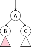
Before describing the corrective procedure, which is called percolate up, let's illustrate the key step. In the diagram on the right A is an existing node with its old value. It doesn't matter if A is a right or left child. We have just replaced the value in either B or C with the new inserted value (by symmetry, assume we just changed B. The reason we aren't finished is that the new value in B is less than the value in A. So we swap these two values and now they are in the right order: the value in A is smaller than the value in B. What is the effect on the rest of the tree?
Let's begin. We added a leaf and want to put the new value V in this new leaf. The problem is that V might be smaller than the value in the parent. If so we swap: The value in the parent goes into the new leaf and we try to put V in the parent. As mentioned this reduces the value in the parent so can't violate heap order with respect to children.
The problem is that V might be smaller than the value in the parent's parent, in which case we have moved up one level in the tree and swap again. At the worst we reach the root which has no parent and thus no violation is possible.
On the board start with an empty tree and insert, in this order, the values 1, 2, 3, 4, 5, ... too easy!
On the board start with an empty tree and insert, in this order, the values 100, 90, 80, 95 (if this were 90, would have two nodes with the same value and would not have caught this), 85, 75, 110 (if 100, would have undetected duplicate), 60.
The situation is as follows.
We know which value to remove (the min is in the root) and we know
which node to delete (the last
leaf)?
Why not simply put the value from the last leaf into the now
valueless root.
Alas, it is very likely too big.
We have basically the same situation as before. For that reason the diagram on the right is the same. The difference is that now the value in A is the one that has changed and is possibly violating the heap order property and we therefore move down the tree. Indeed the procedure is called percolate up. If the value in A is less than the values in the two children, we are done. If not swap the value in A with the smaller of the values in the two children. Say that is the value in B (the case where it is the value in C is symmetric). So now the smallest of the values previously in A, B, or C is in A so these three nodes satisfy the heap order property. What about the rest of the tree.
Thus each iteration fixes everything at its level and above, pushing any problem down one level of the tree. Eventually, B is a leaf and the red triangle is empty so there is no problem remaining.
On the board keep applying delete min to the example constructed previous until the empty tree arises.
On the board do an example with duplicates. For example, redo the previous insert example using the hints to duplicate.
To decrease an item's value just change the value and then percolate up.
Similarly, increasing the value requires a percolate down.
Deleting a specific element can be accomplished by decreasing it's value below that of any other and then doing deleteMin
Start Lecture #20
Remark: What about reading day for lunch?
Remark: Lab 3 assigned. It is due in 2 weeks and is on the web.
Given N values, we can certainly produce a heap by doing N insert() calls. This would require time O(Nlog(N)) in total. In fact we can do better because we know that there will not be any deleteMin() operations intervening. Thus we do not have to first produce a heap with 1 element, and then a heap with 2 elements, and then a heap with 3 elements, etc.
The following algorithm takes an array with N values and converts it to a heap in only O(N) time. The idea is quite simple. As always we can view the array as a tree via
To obtain the order property we start with the highest numbered slot and percolate it down (this will be a no-op since the highest numbered slot must be a leaf and thus can't go down). Then we percolate the next-to-highest numbered slot, and continue until we reach the lowest numbered slot, which is the root
Draw some pictures on the board to show that the result has the heap order property and thus is a heap.
Each percolate down requires time proportional to the height of the node in question. As noted above the tree satisfies the structure property, i.e. it is a complete binary tree. The key to understanding why buildHeap() requires only O(N) time is that the sum of the heights in a complete binary tree is O(N).
This result is proved by a fairly simple counting argument, but we shall not do it.
A slightly modified version of the BinaryHeap class from the author's website is here Note the following points.
Read.
Sorting is very important for data sets that are fairly stagnant, i.e., that remain in sorted order through many accesses. For example, imagine a data set where inserts, deletes, and updates to keys are very rare compared to retrievals and data (not key) updates.
Sorted items can be kept in an array (of objects) and found by binary search (check the middle element, dividing the problem in half). This gives O(log(N)) retrieval cost. An AVL tree matches this big-Oh time but is a little slower, more complicated, and requires space for pointers.
Batch processing of a sorted set of updates can be done in O(N) time assuming each update is O(1).
static void bubbleSort (int[] arr) {
  for (int i=0; i<arr.length-1; i++)
    for (int j=i+1; j<arr.length; j++)
      if (arr[i].compareTo(arr[j]) > 0) {
        int tmp = arr[i];
        arr[i] = arr[j];
        arr[j] = tmp;
      }
}
For uniformity, we assume the problem is to sort an array of objects in a class that implements comparable (actually, we assume that there is a superclass that implements comparable). We also assume that the length of the array is the number of elements we are to sort, i.e., the array is full. So all our algorithms take just one parameter, the array to sort.
There are a number of very easy sorting algorithms that take O(N2) time. The one I use most often for small arrays is shown on the above right.
static void easySort (int[] arr) {
  boolean more;
  do {
    more = false;
    for (int i=0; i<arr.length-1; i++)
      if (arr[i].compareTo(arr[i+1]) > 0) {
        more = true;
        int tmp = arr[i];
        arr[i] = arr[i+1];
        arr[i+1] = tmp;
      }
  } while (more);
}
Perhaps even simpler than my bubbleSort() would be to have an inner loop that checked all adjacent elements and swapped them if they were out of order. A pair of elements that are out of order are called an inversion. We also have an inner loop that keeps going until the outer loop does no swaps. Such a sort is on the immediate right.
Both of these sorts are quite inefficient, even among the O(N2) sorts, because both do three-instruction swaps for each inversion. We will soon see insertion sort, which is a little better since it removes some inversions by one-instruction shifts.
So that the examples above would not be too wide, they each sort only integers. Much better would be a generic version with header line
public static <T extends Comparable<? super T>> void bubbleSort (T[] arr) {
and with tmp declared to be of type T.
First I should explain the name insertion. Instead of being handed an array to sort, imagine that you are given name tags to alphabetize and you are given them one at a time with a significant time delay between each.
public static <T extents Comparable <? super T>>
void insertionSort (T[] a) {
  int j;
  for (int i=1; i<a.length; i++) {
    T tmp = a[i];
    for (j=i; j>0 && tmp.compareTo(a[j-1])<0; j--)
      a[j] = a[j-1];
    a[j] = tmp;
  }
}
To start you are given the first tag You accept it and it becomes a
sorted pile of one tag.
Then you are given a second tag, which you put in the right place in
the pile.
After about five of these, you realize that your action is to
insert one tag into the pile of already sorted tags.
The code on the right does essentially the same thing. The new tag (i.e., object of type T) is a[i]. We start p at 1, not 0, because as mentioned above there is nothing to do when you insert a tag in to an empty pile.
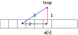
This is another O(N2) sort. As mentioned above, it is a slight improvement over the previous two since, if the new value (a[i]) belongs early in the array, we don't do a bunch of three-statement swaps. Instead we do a bunch of one-statement assignments.
Specifically, as indicated in the diagram, in each outer iteration, we first move a[i] away, then slide over a bunch of a[j]'s, and finally insert the old a[i] in its proper location. It is the sliding that consists of one-statement assignments.
Homework: 7.2
Theorem: The average number of inversions in an array of N distinct elements is N(N-1)/4=O(N2).
Proof: This surprised me for being so easy since it is an average case analysis. For an N-element array, there are exactly N(N-1)/2 pairs that could possibly be inversions. Couple each N-element array with its reverse (i.e., the reverse has same elements as the original, but in the reverse order). For each pair of elements, the values are in order for one of the arrays and out of order for the other. Thus for the two arrays, there are N(N-1)/2 inversions which gives N(N-1)/4 on average.
Corollary: Any algorithm that sorts by exchanging adjacent elements requires Ω(N2) steps on average.
Corollary: Any algorithm that sorts by exchanging adjacent elements requires Ω(N2) steps in the worst case.
Note that insertion sort implicitly exchanges adjacent elements. That is, when it swaps elements that are k apart, it takes Θ(k) (very short) steps.
Thus to improve on quadratic behavior, i.e. to require only o(N2) time with a comparison based sort, we must sometimes compare non-adjacent elements.
public static <T extents Comparable <? super T>> void
insertionSort (T[] a) {
  int j;
  int gap=1;
  for (int i=gap; i<a.length; i++) {
    T tmp = a[i];
    for (j=i; j≥gap && tmp.compareTo(a[j-gap])<0; j-=gap)
      a[j] = a[j-gap];
    a[j] = tmp;
  }
}
This algorithm (named after its inventor) uses the above results in that it does sometimes compare far away values. Shellsort is in a sense a variation on insertion sort, but this is a little hidden in the book. I will try to make the relationship clearer.
The code on the right is the same as insertion sort. The only change is that a bunch of 1's were changed to gap's, but gap is always 1.
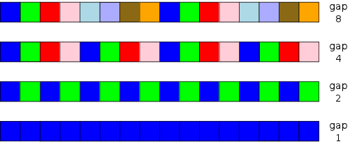
The idea of shellsort is that we put an outer loop around this code changing gap each iteration. The code is just below but first look at the picture on the right, which has a.length==16.
The first row shows an execution with gap==8. This execution does insertion sort on the dark blue squares. If you pick at the code below you will see that the first iteration of the outer loop does exactly what was just described. The next iteration does insertion sort on the green squares; the next on the red squares; and the last iteration does insertion sort on the orange squares.
public static <T extents Comparable <? super T>> void
shellSort (T[] a) {
  int j;
  for (int gap=a.length/2; gap>0; gap/=2)
    for (int i=gap; i<a.length; i++) {
      T tmp = a[i];
      for (j=i; j≥gap && tmp.compareTo(a[j-gap])<0; j-=gap)
        a[j] = a[j-gap];
      a[j] = tmp;
    }
}
Note that, providing the last iteration has gap=1, the code will sort correctly since this last iteration would be just insertion sort, which we know sorts correctly any array so can clean up whatever mess the previous iterations left around.
The code on the right implements this idea using the specific choice of gaps employed by Shell himself. Although this does often work better than insertion sort, it is actually a poor choice from a theoretical view. In fact, with Shell's gaps, shellsort is still an O(N2) algorithm.
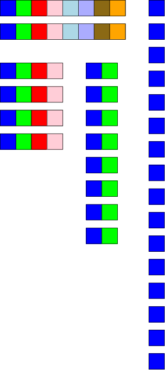
You can think of shellsort and laying out the 1D array as a 2D matrix and just sorting each column. Then you lay it out again with fewer, but taller, columns and repeat.
This 2D column-based interpretation is illustrated on the right for the same gap sequence as in the diagram above (i.e., Shell's sequence for an array with 16 elements). The upper left 2D view indicates the execution during the first iteration, i.e., when gap==8. Note that each column is monochromatic, so this iteration does indeed sort the columns. The squarish picture below illustrates gap==4 and again each column. The same result holds for the other two view, which illustrate gap==2 and gap==1.
As mentioned, Shell's choice of gaps gives poor performance in the worst case. A much better choice of gaps is 1, 3, 7, ... 2k-1 (in the reverse order), as discovered by Hibbard. Considering how similar Shell's and Hibbard's gaps appear to be, it is surprising to learn that the latter improves the worst case time to O(N3/2).
Apparently the gap sequence found to date with the
smallest (i.e., best) big-Oh time is (the reverse of) 1, 2, 3, 4, 6,
9, 8, 12, 18, 27, 16, 24, ... .
This mysterious sequence was found by Robert Sedgewick and achieves
Θ(N(log(N))2) sorting time.
To quote Sedgewick
The increment sequence is formed by starting at 1, then proceeding
though the sequence appending 2 and 3 times each increment
encountered.
Homework: 7.4 (This means show the result after each increment is used)
The book points out that heapsort (based on the binary heap we
learned last chapter) is the first sorting method we have
encountered with O(Nlog(N)) big-Oh time.
Maybe.
We didn't note it at the time, but given N elements you can
put them in an AVL tree in O(Nlog(N)) time (each of N
inserts take O(log(N)) time).
Then you can retrieve the sorted values in O(log(N)) time by
performing an inorder traversal.
Returning to heapsort itself, we can use buildHeap() to produce a heap and then perform deleteMin repeatedly to retrieve the elements in sorted order. The first step is O(N), the second O(Nlog(N)), and the total therefore is O(Nlog(N)).
The only problem is space (i.e., the memory used). We are given the elements in one array and then put then into a second array, which we turn into a heap. Then we repeatedly perform deleteMin on this heap putting the results back in the original array.
This procedure uses a work array
(for the heap) that is the
same size as the input so requires Θ(N)
extra space (i.e., memory over and above that used
for the input itself).
We can do better!
The first part is very easy. Perform buildHeap() on the original array. But the second part seems hard: We must extract the minimums and put them back into the same array without messing up the remaining heap.
The key observation enabling us to accomplish this act is that we always have exactly N values: as we iterate deleteMin() the heap gets smaller and the number of sorted values gets larger. At first all N values are in the heap; at the end all N are sorted. After k steps the first N-k slots are in the heap and the last k contain the sorted values. So it does seem possible to not use more than N values.
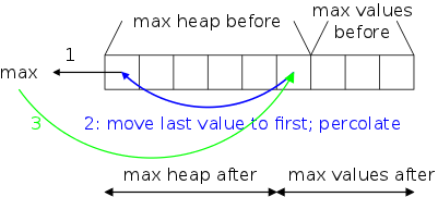
See the diagram on the right for the solution.. The first observation is that we use buildHeap() to construct a max heap instead of our usual min heap. This means that we will be iterating deleteMax().
Recall that deleteMax() begins by removing the first element of the array, which is the root of the tree, i.e., is the maximum value. Then the element in the last slot is moved to the first. Finally, we execute a percolate down on the first element. When percolate concludes we now have a max heap that no longer uses the last slot. We place the previously-extracted max into this free slot and smile.
Homework: 7.11, 7.12
static void merge (long[]ans,long[]a,long[]b) {
  int i=0, j=0, k=0;
  while (i<a.length && j<b.length)
    if (a[i] <= b[j])
      ans[k++] = a[i++];
    else
      ans[k++] = b[j++];
  while (i<a.length)
    ans[k++] = a[i++];
  while (j<b.length)
    ans[k++] = b[j++];
}
Another O(Nlog(N)) algorithm. This is quite easy to describe, once you know what merging is. Given two sorted lists it is not hard (and very fast) to merge them into a third sorted list:
A non-generic merge is on the right.
Imagine two sorted decks of cards face up so that you can always see the top card on each deck. Then to merge them into one sorted deck, keep picking up the smaller of the two visible cards until one of the input piles is empty. Then take all the remaining cards from the non-empty input deck.
public static void mergeSort1 (long[]a) {
  if (a.length < 2)
    return;
  int split = a.length / 2;
  long[] left  = new long[split];
  long[] right = new long[a.length-split];
  for (int i=0; i<split; i++)
    left[i] = a[i];
  for (int i=split; i<a.length; i++)
    right[i-split] = a[i];
  mergeSort1(left);
  mergeSort1(right);
  merge(a,left,right);
}
Giving a procedure for merging, mergeSort(T a) proceeds as follows
As usual we need a base case so that the recursion stops eventually. For mergeSort() the base case is that sorting an array with 0 or 1 element is a no op.
The code on the right is a simple implementation. I believe it is clearer than the one in the book; but the book's uses considerably less memory, as we shall see later.
Start Lecture #21
Remark: Lab2 has been graded (probably for a while). I just sent an email asking Radhesh to send each of you your score.
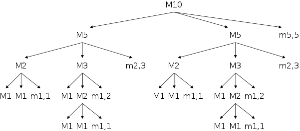
Before worrying about space efficiency, let's see how the implementation actually works.
On the right is the call graph for a call to mergeSort1() with an array of size 10. Each M represents a call to mergeSort1() and each m represents a call to merge() and gives the size of the two input arrays.
Go over the call graph on the board. That is, do a sort of 10 elements and follow the flow.
Looking at the code for mergeSort1() above we see that
there are two loops each copying about half the current matrix
a into new about half-size arrays left
and right.
If we choose the original array to be of length a power of two, we
can erase the two about
s in the previous sentence.
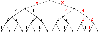
The diagram on the right shows the situation for an initial 16-element array. The top of the tree illustrates that initially the 16 elements are copied to two 8-element arrays. The next row shows each of the 8-elements arrays being copied to two 4-element arrays, etc. In each row there are a total of 16 elements copied and there are four rows. Note that each of the copies is to a different array so the result is 64 copies to 64 additional objects.
If we let N=2k be the size of the original array, then each row copies N elements and there are k=log(N) rows. Thus the mergeSort1() implementation above performs Nlog(N) copies and needs Nlog(N) extra objects.
For a general N, not necessarily a power of two, the result is essentially the same, but is a little messier to count. We will not do the exact calculation, but will state that for any N, mergeSort1() needs Θ(Nlog(N)) extra objects and performs Θ(Nlog(N)) copies.
Note that many of these objects can be freed by the system so the actually memory used at any point is less, but the storage allocation and reclamation does cost. It seems to me that at the point just before the last (i.e., rightmost) 1-element MergeSort1() returns, the arrays shown in red above are all still resident.
I ran a test, and the time required to compile the program, generate an array with 50,000,000 elements, sort it, and check the results was 24 seconds on my laptop. The actual code used is here.
We can reduce the extra memory from Θ(Nlog(N)) extra objects, to Θ(N) extra objects by making one extra (full size) array and using it at every level of the tree.
This requires coding changes.
public static void mergeSort2(Long[a]) {
  long[] tmpA = new long[a.length];
  mergeSort2(a, tmpA, 0, a.length-1);
}
private static void
mergeSort2 (Long[]a, Long[]tmpA, int left, int right) {
  if (right <= left) 	// one or zero items
    return;
  int split = (left+right)/2; // last entry first half
  mergeSort2(a, tmpA, left, split);
  mergeSort2(a, tmpA, split+1, right);
  merge(a, tmpA, left, split, right);
}
The public method simply creates the temporary array and calls the internal (recursive) method specifying the entire array.
The internal method is given both the original and temporary array as well as the range of the original array it is responsible for sorting. The sorted result is placed back in the same portion of the original array. As before the method has three steps
private static void
merge (long[]a, long[]tmpA,int left,int split,int right){
// left half = left..split    right half = split+1..right
  int i=left, j=split+1, k=left;
  while (i<=split && j<=right)
    if (a[i] <= a[j])
      tmpA[k++] = a[i++];
    else
      tmpA[k++] = a[j++];
  while (i<=split)
    tmpA[k++] = a[i++];
  while (j<=right)
    tmpA[k++] = a[j++];
for (i=left; i<=right; i++) // copy tmpA back to a
  a[i] = tmpA[i];
}
In this implementation (largely from the book) it is the merge() method that does the copying. Specifically, it merges the two just-now-sorted pieces of the original array into the corresponding range of the temporary array and the copies the result back.
Although mergeSort1() and mergeSort2() are fundamentally the same, I find the former a little easier to read.
Counterbalancing the last subjective statement is the objective measurement showing that the second version is faster. To create, sort, and check the same 50,000,000 array now takes only 17 seconds.
The copy back at the end of merge() can be eliminated by doing an initial copy in the public method and flip flopping the a and tmpA arrays. With this improvement the program takes 14 seconds.
Homework: 7.15
Remark: I added other homework problems for chapter 7. They are not due in but you might them helpful.
This is a very popular sorting algorithm, used in a number of standard libraries. However, its worst case time is not good, O(N2). Quicksort is popular because, if implemented well, it is very fast in practice. Like mergesort, quicksort is basically a divide and conquer algorithm.
Assuming S is the given set of elements, quicksort proceeds as follows.
As we shall see in the code examples to follow, elements equal to the pivot are often placed into one or both of the other groups (the one chosen pivot is kept separate).
public static void quickSort1 (long[]a) {
  quickSort1(a, a.length);
}
private static void quickSort1(long[]a, int n) {
  if (n < 2)
    return;
  long pivot = a[0];
  long[] lessEql = new long[n];
  long[] greater = new long[n];
  int lessEqlN=0, greaterN=0;
  for (int i=1; i<n; i++)
    if (a[i] <= pivot)
      lessEql[lessEqlN++] = a[i];
    else
      greater[greaterN++] = a[i];
  quickSort1(lessEql, lessEqlN);
  quickSort1(greater, greaterN);
  for (int i=0; i<lessEqlN; i++)
    a[i] = lessEql[i];
  a[lessEqlN] = pivot;
  for (int i=0; i<greaterN; i++)
    a[lessEqlN+1+i] = greater[i];
}
The above description is incomplete. In particular, it is far from clear how to best accomplish steps 2 and 3. Although it is not hard to find correct implementations, to get a high speed sort it is important to choose an efficient implementation.
For example on the right is the easiest implementation I could come up with. It has the virtue of being easy to understand, but it performs quite poorly. This code gets a java.lang.OutOfMemoryError exception sorting 100,000 elements on the same laptop that sorted 50,000,000 elements with mergesort.
The biggest inefficiency in the code is the creation of separate arrays for each sublist. As we shall see below a serious implementation does the partitioning in place.
As mentioned above, it is very easy to pick a correct pivot, i.e., one for which the algorithm sorts correctly. However, some choices are considerably better than others. The goal in choosing the pivot is to have about as many element bigger than the pivot as there are elements less than the pivot.
A pragmatically poor choice is to pick the first (or last) element of the array. The reason this is a poor choice is that, in practice, it is not rare to sort an array that is (almost) already sorted. In the extreme case of a completely sorted array, choosing the first (or last) element as the pivot will result in the third (or first) group being empty. The effect is analogous to a binary search tree in which no node has a left child.
The low-quality example above uses this method. The runs discussed were with the pseudo-random input we used before; presumably it would be even worse if I gave it sorted input
The book didn't mention choosing the middle element of the original array, but that is a reasonable choice. For example, given an array with these 11 values
6, 8, 20, 30, 0, 7, 15, 18, 2, 1, 4
the middle element is element number 6, which is a 7.
Choosing an element of the array at random is a safe choice for the pivot, but is somewhat slow.
The current favorite is to examine three array elements, the first, the last, and the middle, and then chose the median of these three values. For example, given the same 11 values as above, namely
6, 8, 20, 30, 0, 7, 15, 18, 2, 1, 4
the first/last/middle are 6/4/7 and the median of these three is 6,
which would be chosen as the pivot.
Start Lecture #22
For good performance it is important to do the partitioning in place. The big gain is that no extra arrays are created; instead the recursive call specifies a range of the original array to sort. The basic in-place partitioning method is simple, but care is needed as slight changes can reduce performance considerably.
big onesto the right of all
small ones. Big and small mean respectively bigger and smaller than the pivot.
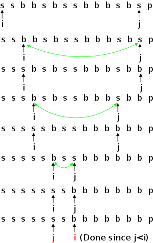
First we assume there are no duplicates, which implies that once the pivot is moved away, no remaining element equals the pivot. It also means that when comparing distinct elements, we know they can't have equal value, but this turns out not to be important.
The idea for step 2 is to use two pointers one starts at the left end and moves right, the other at the right end and moves left. The first pointer stops when if encounters a big element and the second stops when it encounters a small element. If at this point, the first counter is still to the left of the second, the corresponding elements are swapped and the procedure continues.
The diagram on the right illustrates step 2. Rather than show specific values, I just indicate whether the given value is smaller than the pivot (s), is bigger (b), or is the pivot (p).
The transition from row one to row two of the picture illustrates moving the pointers. Note that in row two, i points to a b and j points to an s. The double headed green arrow indicates that these elements are to be swapped, which leads to row three.
At this point we again move the pointers leading to row four. Another pair of swapping and moving yields rows five and six.
The final pair of swapping and moving results in rows seven and eight, at which point we terminate instead of swapping since the left pointer is now to the right of the right pointer.
What should we do if, while moving the left and right pointer, we encounter a value equal to the pivot? Should the counter move or stop? Best would be to have all the pivots accumulate in the center and then not sort them again. But this turns out to slow down partitioning too much.
We do not want to either move all the pivots to the left or move all of them to the right since would make the chosen side larger and, as usual in a divide and conquer algorithm, we want the division to be into roughly equal sized pieces.
As explained in the book, it is better to have each pointer stop when it sees a pivot value. If it turns out that both stop at pivots, a useless swap will be performed. We could test for this case and not swap, but most of the time the test will fail and the overall result is to slow the program.
For small arrays quicksort is slower than insertion sort and due to its divide and conquer approach, quicksorting a large array includes very many quicksorts of small arrays. Thus good programs check the size and switch to special code for small (sub)arrays.
Start Lecture #23
static final int CUTOFF = 10;

public static void quickSort2 (long[]a) {
  quickSort2(a, 0, a.length-1);
}

private static long
median3 (long[]a, int left, int right) {
  int center = (left+right) / 2;
  if (a[center] < a[left])
    swapElements (a, left, center);
  if (a[right] < a[left])
    swapElements (a, left, right);
  if (a[right] < a[center])
    swapElements (a, center, right);
  swapElements (a, center, right-1);
  return a[right-1];
}

private static void
quickSort2 (long[] a, int left, int right) {
  if (right-left <= CUTOFF) {
    insertionSort(a, left, right);
    return;
  }
  long pivot = median3(a, left, right);
  int i = left, j = right-1;
  while (true) {
    while (a[++i] < pivot) ;
    while (a[--j] > pivot) ;
    if (i >= j)
      break;
    else
      swapElements (a, i, j);
  }
  swapElements (a, i, right-1);
  quickSort2 (a, left, i-1);
  quickSort2 (a, i+1, right);
}

private final static void
swapElements (long[] a, int i, int j) {
  long tmp = a[i];
  a[i] = a[j];
  a[j] = tmp;
}

private static void
insertionSort (long[] a, int left, int right) {
  int j;
  for (int i=left+1; i<=right; i++) {
    long tmp = a[i];
    for (j=i; j%gt;left && tmp<a[j-1]; j--)
      a[j] = a[j-1];
    a[j] = tmp;
  }
}
First we establish the cutoff value below which insertion sort will be executed.
Since all the work will be performed on the original array, most of the routines will require three inputs: the array and the left and right bounds of interest. The one exception is the public interface, which accepts just the array and gets the ball rolling by calling the workhorse private routine, specifying the entire range of indices.
The median3() method examines and sorts the first, last, and middle element. That is it alters the matrix as well as calculating the pivot. The new middle element is the pivot. It is put in the penultimate slot (the value in the last slot is at least as big) and its value is returned.
The internal quickSort2() method, first checks if the range is small enough for insertionSort(), then lets median3() find the pivot, and then proceeds to partitioning the array.
Due to the alterations performed by median3(), the partitioning strategy need only be applied to the range left+1..right-2. However, the range used is left..right-1. But note that the subsequent increments to i and decrements to j are preincrements/decrements, so the correct values are used for the first iteration. The book mentions a subtlety explaining why apparently similar code can loop forever.
After the outer loop is broken out of, the pivot is swapped with the value at the right moving counter and the two subarrays are recursively sorted.
The swapElements() method simply interchanges two slots in the matrix.
The insertionSort() method is an old friend. The only change is that instead of acting on slots 0..a.length, it is restricted to left..right.
Use the code on input Y E S A T E E N O A V B K and show the steps on the board.. Don't forget to check with sheets done at home to avoid typos.
Homework: 7.19
Do on the board an example with all keys equal.
Do on the board an example with all keys equal and not stopping when a value equal to the key is found.
Do on the board an example with all keys equal and not stopping i when a value equal to the key is found but stopping j when a value equal to the key is found. This is the essence of 7.22.
Homework: 7.24. The idea is to at each recursion, make the larger piece as large as possible (the same as making the smaller piece as small as possible).
When run on the same 50,000,000-entry matrix, quickSort2() required 17 seconds, which is slower than the fastest mergesort routine we developed last section. Since I expected quicksort to be faster than mergesort, I replaced swapElements() calls with the 3 statement body as mentioned in the book and then eliminated the longer recursive call (solving problems 7.25 and 7.26). This implementation reduced the time to 14 seconds, matching the fastest mergesort.
The end of the mergesort section asserts that for primitive types (such as long, which I used), the Java library uses quicksort, which suggests that it is faster. Perhaps there are more speed tricks to play; quicksort is notoriously sensitive to the exact implementation. If anyone tinkers and finds a faster version, I would appreciate knowing.
There are several mathematical notions of
average
.
The most common is probably the
arithmetic mean, which is the familiar
add them up, and divide by how many
.
Two other means are also used.
In this section we are interested in (a generalization of) another average, namely the median. The median of n numbers is defined as follows.
For completeness, the mode is the most common element. It is not defined if several elements tie for most common.
Consider the following list of integers
3 5 7 2 4 3 9 3 9 4 2 5 6
When sorted this becomes
2 2 3 3 3 4 4 5 5 6 7 9 9
The list has 13 elements so
If, for example, n=23, then the median is the 12th-largest. But we might want the 5th- or 20th-largest even if n=23. The general problem of finding the kth-largest for arbitrary k is often called selection.
Note that the result is a single value chosen from the array, not a sorted version of the entire array. The algorithm for selection is basically a simplified version of quicksort. It proceeds as follows.
When we are finished, the desired element (the kth-largest) is in slot k-1 of the array. Note that part of the array is unsorted.
Naturally, we need a base case to break the recursion, and for efficiency when the subarray is small, we use insertion sort.
Start Lecture #24
public class QuickSelect {
  static final int CUTOFF = 10;

  public static void quickSelect (long[]a, int k) {
    quickSelect(a, 0, a.length-1, k);
  }

  private static void
  quickSelect (long[] a, int left, int right, int k) {
    if (right-left <= CUTOFF) {
      insertionSort(a, left, right);
      return;
    }
    long pivot = median3(a, left, right);
    int i = left, j = right-1;
    while (true) {
      while (a[++i] < pivot) ;
      while (a[--j] > pivot) ;
      if (i >= j)
	break;
      else
	swapElements (a, i, j);
    }
    swapElements (a, i, right-1);
    if (k<=i)
      quickSelect (a, left, i-1, k);
    else if (k>i+1)
      quickSelect (a, i+1, right, k);
  }

  // median3, swapElements, insertionSort unchanged

  public static void main(String[]args) {
    final int n=50000000, p=37;
    long[] a = new long[n];
    int val = p;
    for (int k=333; k<n; k+=n/9) {
      for (int i=0; i<n; i++)
	a[i] = (long)(val = (val+p)%n);
      quickSelect(a, k);
      System.out.println
        ("The " + k + "th largest is " + a[k-1]);
    }
  }
}
Due to its similarity with quickSort(), we call the method using the above algorithm quickSelect(). As with quickSort(), quickSelect() begins by defining the size below which an insertion sort is to be used.
The public method quickSelect() takes two parameters, the array containing the elements and k, specifying which value we are seeking. Parts of the array will have been sorted so if the original array is required, the user must make a copy before calling quickSelect().
Again similar to quickSort(), the workhorse is a private method that has two additional parameters specifying the interesting range of the array. The workhorse begins identically to the one in quickSort(): First we see if the subarray is so small that an insertion sort should be used. Then median3() is called. This routine is identical to the version used in quicksort and is therefor not shown.
The partitioning step is also identical to the quicksort version as is the subsequent swap to place the pivot between the two subarrays.
The significant difference follows. Only one (or zero, if the pivot is the desired value) recursive invocation occurs, the subarray not contained the sought for value is left unsorted. Also if the larger subarray is chosen, the value of k must be adjusted to account for the values in the unchosen array and the pivot.
In addition to median3(), the swapElements() and insertionSort() methods are unchanged from the versions in the quicksort program and thus are not shown.
The main() method does 9 tests seeking different values in the same array.
The workhorse quickSort() method basically does the following steps when given a subarray of size N (ignore the use of insertion sort for small arrays).
The workhorse quickSelect() method is similar.
Lets consider the best case where the pivot divides the array in half. For simplicity we will start with an array of size 32=25 and pretend that the subarrays are of size 16 (really the pivot takes a slot so one subarray is 15).
Let T(N) be the time needed for quicksort to sort an array of size N in this favorable case. Then looking at the three steps above we see that.
T(N) = a + bN + 2T(N/2)
If we let S(N) be the time for quickselect and again look
at the three steps we see something very similar.
S(N) = a + bN + S(N/2)
This is sloppy a and b would not be the same for
the two algorithms.
It looks like quickselect is about two times faster so in big-Oh notation they should be the same. But that is wrong! Letting N=32 we see for quicksort:
    T(32) =   a +  32b +  2T(16)
          =   a +  32b +  2(a + 16b + 2T(8)) =   a +  32b +  2a + 32b +  4T(8)
          =  3a +  64b +  4(a +  8b + 2T(4)) =  3a +  64b +  4a + 32b +  8T(4)
          =  7a +  96b +  8(a +  4b + 2T(2)) =  7a +  96b +  8a + 32b + 16T(2)
          = 15a + 128b + 16(a +  2b + 2T(1)) = 15a + 128b + 16a + 32b + 32T(1)
          = 31a + 160b + 32C  ~  (a+C)N + bN(log N), which is Θ(NlogN).
But for quickselect we have
    S(32) =  a + 32b + S(16)
          =  a + 32b + (a + 16b + S(8)) =  a + 32b + a + 16b + S(8)
          = 2a + 48b + (a +  8b + S(4)) = 2a + 48b + a +  8b + S(4)
          = 3a + 56b + (a +  4b + S(2)) = 3a + 56b + a +  4b + S(2)
          = 4a + 60b + (a +  2b + S(1)) = 4a + 60b + a +  2b + S(1)
          = 5a + 62b + D  ~  a(logN) + bN + D, which is Θ(N).
We have seen two sorting algorithms with Θ(NlogN) worst-case complexity: heapsort and mergesort. Can we do better?
It a sense, to be made more precise shortly, the answer is no!
Assume we are sorting an array of N distinct integers stored in an array in slots 1..N.
To begin let N=2 and let the initial value in slot 1 by x1 and the initial value in slot 2 be x2. There are two distinct answers depending the values of x1 and x2. Either the two values are swapped or they are left in their original slots.
For N=3, there are six possible answers. The three values can be in one of these six orders: (x1,x2,x3), (x1,x3,x2), (x2,x1,x3), (x2,x3,x1), (x3,x1,x2), or (x3,x2,x1).
For general N there are N! different answers.
This means that there must be at least N! different executions that can occur.
To show the possible execution sequences we make use of a decision tree. Nodes represent points in an execution and arcs show the effects of decisions based on comparisons. As we proceed with an execution and decisions are made (if vs then, repeat a while or end it, continue a for or leave it, etc) the number of possible answers is reduced. Eventually, we reach an end of the execution and have determined the answer.
The diagram below corresponds to the three element sort we use in quicksort and quickselect. What is shown is how to narrow down the choices, we do not show the actual swapping of elements. In the beginning there are six possibilities.
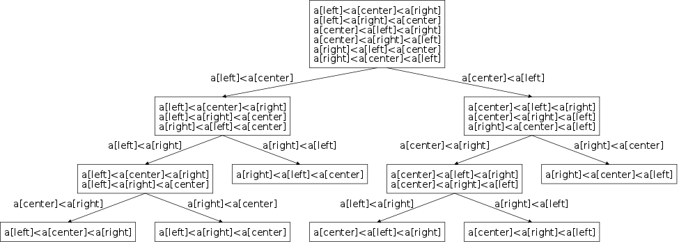
Assume that all we can do to reduce the possibilities is to compare two elements, which is all our sorts ever do. After you ask enough questions (in this case three questions suffices), there is only one possibility and hence you can generate the answer with no more questions.
The key points to note are that
Our goal is to first show that for N values and hence N! leaves, the tree will have height at least log(N!). Our second goal will be to show that log(N!) is Ω(NlogN). Then we will put these two observations together and see than any comparison-based sorting algorithm will require Ω(NlogN) time in the worst case, showing that mergesort and heapsort are optimal in this sense.
Theorem: A binary tree of height h has at most 2h leaves.
Proof: The formal proof is via induction (a height h binary tree is just a (non-leaf) root and two height h-1 subtrees). But I think it is clear without induction. How would you make a binary tree of height 3 have as many leaves as possible? You would make all levels full so all the leaves are at the bottom and there are 23 of them.
Corollary: Any binary tree with k leaves has height at least log(k).
Corollary: Any decision tree for sorting N values has N! leaves and hence has height at least log(N!), which was our first goal.
Assume N is even (odd is essentially the same; just a little messy). Then the first N/2 factors in N! are each at least N/2. Thus, N! > (N/2)(N/2). Hence log(N!) > (N/2)log(N/2), which is Ω(NlogN), accomplishing the second goal.
From the two goals we see that any decision tree for sorting N values has height Ω(NlogN). This means there is a leaf that is Ω(NlogN) comparisons away from the root and each of these comparisons requires an instruction to execute.
The reason I want to cover this material is not because bucket sort is excitingly clever; it is actually quite trivial. The importance of this material is that the efficiency of bucket sort shows a limitation in the above lower bound result. Specifically, bucket sort emphasizes the importance of the restriction to comparison-based sorting.
static final int MAXVALUE = 1000;
static int[] count = new int[MAXVALUE+1];
public static void bucketSort (int[]a) {
  for (int val=0; val<=MAXVALUE; val++)
    count[val] = 0;
  for (int i=0; i<a.length; i++)
    count[a[i]]++;
  int i = 0;
  for (int val=0; val<=MAXVALUE; val++)
    for (int j=0; j<count[val]; j++)
      a[i++] = val;
}
Bucket sort assumes that the values in the array are known to be in a bounded range. The code on the right uses the range 0..MAXVALUE.
We count how many occurrence there are of all the values in this range and then just put the appropriate values back into the array.
Let N be a.length, the number of numbers to sort and let M be MAXVALUE+1, the number of possible values.
The reason bucket sort is faster than the lower bound of Ω(NlogN) is that bucket uses a more powerful operation that a simple binary comparison. The statement count[a[i]]++; is actually a multi-way decision. Since the slot that is updated depends on the value of a[i], M possible actions can take place.
Start Lecture #25
The sorting algorithms we have considered so far, assumed the data could fit in memory. For very large datasets, this is not practical. Once the data is on disk (the book considers tapes; but today disks are much more common), access is very slow so we want to access a bunch of data at once and deal with it as much as possible, before writing it back to disk.
The book considers tapes so is very worried about how many files there are since a tape drive is need for each file. Today, external sorts are disk based so the problem with many files is not important. However, the main problem, slow access, is still present. Also high-performance modern external sorts try to uses multiple disk drives in parallel.
Much of this material is from Wikipedia.
The basic idea is fairly simple. Assume you have a huge dataset (100GB) that is much bigger than the available RAM (3GB). Then proceed as follows.
We learned some pretty hot sorts. I improved my timing to just measure just the sorting time and both quicksort and mergesort need under 5 seconds to sort 50,000,000 longs.
Insertionsort is quite simple, but not good for large problems.
Mergesort has a lot going for it. It's worst cast time is O(NlogN), which is the best possible for comparison-based sorting. It is not a large program and the book says it is the fastest sort on Java objects.
Quicksort is rather subtle, but it is claimed to be the fastest on Java primitive types, although my experiments showed that mergesort was equally good.
Heapsort is another O(NlogN) sort, but is slower in practice than either quicksort or mergesort.
External sorting is based on mergesort.
The End: Good luck on the final!