Operating Systems
Start Lecture #11
3.7 Segmentation
Up to now, the virtual address space has been
contiguous.
In segmentation the virtual address space is divided into a number
of variable-size segments.
One can view the designs we have studied so far as having just one
segment, the entire process.
- Among other issues this makes memory management difficult when
there are more that two dynamically growing regions.
- With two regions you start them on opposite sides of the virtual
space as we did before.
- Better is to have many virtual address spaces each starting at
zero.
- This split up is user visible.
So a segment is a logical split up of the address space.
Unlike with (user-invisible) paging, segment boundaries occur at
logical point, e.g., at the end of a procedure.
- Imagine a system with several large, dynamically-growing, data
structures.
The same problem we mentioned for the OS when there are more
than two growing regions, occurs as well for user programs.
The user (or some user-mode tool) must decide how much virtual
space to leave between the different tables.
With segmentation
- Eases flexible protection and sharing:
One places in a single segment a unit that is logically shared.
This would be the natural method to implement shared libraries.
- When shared libraries are implemented on paging systems, the
design essentially mimics segmentation by treating a collection
of pages as a segment.
This is more complicated since one must ensure that the end of
the unit to be shared occurs on a page boundary (this is done by
padding).
- Without segmentation (equivalently said with just one segment)
all procedures are packed together so, if one changes in size,
all the virtual addresses following this procedure are changed
and the program must be re-linked.
With each procedure in a separate segment this relinking would
be limited to the symbols defined or used in the modified
procedure.
Homework:
Explain the difference between internal fragmentation and external
fragmentation.
Which one occurs in paging systems?
Which one occurs in systems using pure segmentation?
** Two Segments
Late PDP-10s and TOPS-10
- Each process has one shared text segment, that can
also contain shared (normally read only) data.
As the name indicates, all process running the same executable
share the same text segment.
- The process also contains one (private) writable data segment.
- Permission bits define for each segment.
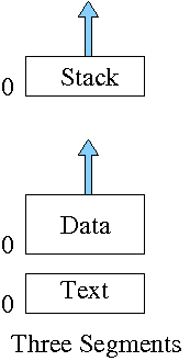
** Three Segments
Traditional (early) Unix had three segments as shown on the right.
- Shared text marked execute only.
- Data segment (global and static variables).
- Stack segment (automatic variables).
Since the text doesn't grow, this was sometimes treated as 2
segments by combining text and data into one segment.
But then the text could not be shared.
** General (Not Necessarily Demand) Segmentation
Segmentation is a user-visible division of a process into
multiple variable-size segments, whose sizes
change dynamically during execution.
It enables fine-grained sharing and protection.
For example, one can share the text segment as done in early unix.
With segmentation, the virtual address has two
components: the segment number and the offset in the segment.
Segmentation does not mandate how the program is
stored in memory.
- One possibility is that the entire program must be in memory
in order to run it.
Use whole process swapping.
Early versions of Unix did this.
- Can also implement demand segmentation (see below).
- More recently, segmentation is combined with demand paging
(done below).
Any segmentation implementation requires a segment table with one
entry for each segment.
- A segment table is similar to a page table.
- Entries are called STEs, Segment Table Entries.
- Each STE contains the physical base address of the segment and
the limit value (the size of the segment).
- Why is there no limit value in a page table?
- Answer: All pages are the same size so the limit is obvious.
The address translation for segmentation is
(seg#, offset) --> if (offset<limit) base+offset else error.
3.7.1: Implementation of Pure Segmentation
Pure Segmentation means segmentation without paging.
Segmentation, like whole program swapping, exhibits external
fragmentation (sometimes called checkerboarding).
(See the treatment of OS/MVT for a review of
external fragmentation and whole program swapping).
Since segments are smaller than programs (several segments make up
one program), the external fragmentation is not as bad as with whole
program swapping.
But it is still a serious problem.
As with whole program swapping, compaction can be employed.
| Consideration | Demand
Paging | Demand
Segmentation |
|---|
| Programmer aware | No | Yes |
| How many addr spaces | 1 | Many |
| VA size > PA size | Yes | Yes |
Protect individual
procedures separately
| No | Yes
|
Accommodate elements
with changing sizes
| No | Yes
|
| Ease user sharing | No | Yes |
| Why invented
| let the VA size
exceed the PA size
| Sharing, Protection,
independent addr spaces
|
| | |
| Internal fragmentation
| Yes | No, in principle
|
| External fragmentation | No | Yes |
| Placement question | No | Yes |
| Replacement question | Yes | Yes |
** Demand Segmentation
Same idea as demand paging, but applied to segments.
- If a segment is loaded, base and limit are stored in the STE and
the valid bit is set in the STE.
- The STE is accessed for each memory reference (not really,
there is probably a TLB).
- If the segment is not loaded, the valid bit is unset.
The base and limit as well as the disk address of the segment is
stored in the an OS table.
- A reference to a non-loaded segment generate a segment fault
(analogous to page fault).
- To load a segment, we must solve both the placement question and the
replacement question (for demand paging, there is no placement question).
- Pure segmentation was once implemented by Burroughs in the B5500.
I believe the implementation was in fact demand segmentation
but I am not sure.
Demand segmentation is not used in modern systems.
The table on the right compares demand paging
with demand segmentation.
The portion above the double line is from Tanenbaum.
** 3.7.2 and 3.7.3 Segmentation With (Demand) Paging
These two sections of the book cover segmentation combined with
demand paging in two different systems.
Section 3.7.2 covers the historic Multics system of the 1960s (it
was coming up at MIT when I was an undergraduate there).
Multics was complicated and revolutionary.
Indeed, Thompson and Richie developed (and named) Unix partially in
rebellion to the complexity of Multics.
Multics is no longer used.
Section 3.7.3 covers the Intel Pentium hardware, which
offers a segmentation+demand-paging scheme that is not used by any
of the current operating systems (OS/2 used it in the past).
The Pentium design permits one to convert
the system into a
pure damand-paging scheme and that is the common usage today.
I will present the material in the following order.
- Describe segmentation+paging (not demand paging) generically,
i.e. not tied to any specific hardware or software.
- Note the possibility of using demand paging (again
generically).
- Give some details of the Multics implementation.
- Give some details of the Pentium hardware,
especially how it can emulate straight demand paging.
** Segmentation With (non-demand) Paging
One can combine segmentation and paging to get advantages of
both at a cost in complexity.
In particular, user-visible, variable-size segments are the most
appropriate units for protection and sharing; the addition of
(non-demand) paging eliminates the placement question and external
fragmentation (at the smaller average cost of 1/2-page internal
fragmentation per segment).
The basic idea is to employ (non-demand) paging on each segment.
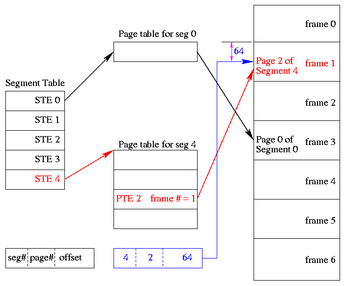
A segmentation plus paging scheme has the following properties.
- A virtual address becomes a triple:
(seg#, page#, offset).
- Each segment table entry (STE) points to the page table for
that segment.
Compare this with a
multilevel page table.
- The physical size of each segment is a multiple of the page
size (since the segment consists of pages).
The logical size is not; instead we keep the exact size in the
STE (limit value) and terminate the process if it references
beyond the limit.
In this case the last page of each segment is partially wasted
(internal fragmentation).
- The page# field in the address gives the entry in the chosen page
table and the offset gives the offset in the page.
- From the limit field, one can easily compute the size of the
segment in pages (which equals the size of the corresponding page
table in PTEs).
- A straightforward implementation of segmentation with paging
would requires 3 memory references (STE, PTE, referenced word) so a
TLB is crucial.
- Some books carelessly say that segments are of fixed size.
This
is wrong.
They are of variable size with a fixed maximum and with
the requirement that the physical size of a segment is a multiple
of the page size.
- Keep protection and sharing information on segments.
This works well for a number of reasons.
- A segment is variable size.
- Segments and their boundaries are user-visible
- Segments are shared by sharing their page tables.
This eliminates the problem mentioned above with
shared pages.
- Since we have paging, there is no placement question and
no external fragmentation.
- The problems are the complexity and the resulting 3 memory
references for each user memory reference.
The complexity is real.
The three memory references would be fatal were it not for TLBs,
which considerably ameliorate the problem.
TLBs have high hit rates and for a TLB hit there is essentially
no penalty.
Although it is possible to combine segmentation with non-demand
paging, I do not know of any system that did this.
Homework: 36.
Homework: Consider a 32-bit address machine using
paging with 8KB pages and 4 byte PTEs.
How many bits are used for the offset and what is the size of the
largest page table?
Repeat the question for 128KB pages.
So far this question has been asked before.
Repeat both parts assuming the system also has segmentation with at
most 128 segments.
Remind me to do this in class next time.
Homework:
Consider a system with 36-bit addresses that employs both
segmentation and paging.
Assume each PTE and STE is 4-bytes in size.
- Assume the system has a page size of 8K and each process can
have up to 256 segments.
How large in bytes is the largest possible page table?
How large in pages is the largest possible segment?
- Assume the system has a page size of 4K and each segment can
have up to 1024 pages.
What is the maximum number of segments a process can have?
How large in bytes is the largest possible segment table?
How large in bytes is the largest possible process.
- Assume the largest possible segment table is 213
bytes and the largest possible page table is 216
bytes.
How large is a page?
How large in bytes is the largest possible segment?
** Segmentation With Demand Paging
There is very little to say.
The previous section employed (non-demand) paging on each segment.
For the present scheme, we employ demand paging on each segment,
that is we perform fetch-on-demand for the pages of each segment.
The Multics Scheme
Multics was the first system to employ segmentation plus demand
paging.
The implementation was as described above with just a few wrinkles,
some of which we discuss now together with some of the parameter
values.
- The Multics hardware (GE-645) was word addressable, with
36-bit words (the 645 predates bytes).
- Each virtual address was 34-bits in length and was divided
into three parts as mentioned above.
The seg# field was the high-order 18 bits;
the page# field was the next 6 bits; and
the offset was the low-order 10 bits.
- The actual implementation was more complicated and the full
34-bit virtual address was not present in one place in an
instruction.
- Thus the system supported up to 218=256K segments,
each of size up to 26=64 pages.
Each page is of size 210 (36-bit) words.
- Since the segment table can have 256K STEs (called
descriptors), the table itself can be large and was itself
demand-paged.
- Multics permits some segments to be demand-paged while other
segments are not paged; a bit in each STE distinguishes the two
cases.
The Pentium Scheme
The Pentium design implements a trifecta: Depending on the setting
of a various control bits the Pentium scheme can be pure
demand-paging (current OSes use this mode), pure segmentation, or
segmentation with demand-paging.
The Pentium supports 214=16K segments, each of size up
to 232 bytes.
- This would seem to require a 14+32=46 bit virtual address, but
that is not how the Pentium works.
The segment number is not part of the virtual address
found in normal instructions.
- Instead separate instructions are used to specify which are
the currently active
code segment
and data segment
(and other less important segments).
Technically, the CS register is loaded with the selector
of the active code segment and the DS register is loaded with
the selector
of the active data register.
- When the selectors are loaded, the base and limit values are
obtained from the corresponding STEs (called descriptors).
- There are actually two flavors of segments, some are private
to the process; others are system segments (including the OS
itself), which are addressable (but not necessarily accessible)
by all processes.
Once the 32-bit segment base and the segment limit are determined,
the 32-bit address from the instruction itself is compared with the
limit and, if valid, is added to the base and the sum is called the
32-bit linear address
.
Now we have three possibilities depending on whether the system is
running in pure segmentation, pure demand-paging, or segmentation
plus demand-paging mode.
-
In pure segmentation mode the linear address is treated as the
physical address and memory is accessed.
-
In segmentation plus demand-paging mode, the linear address is
broken into three parts since the system implements
2-level-paging.
That is, the high-order 10 bits are used to index into the
1st-level page table (called the page directory).
The directory entry found points to a 2nd-level page table and
the next 10 bits index that table (called the page table).
The PTE referenced points to the frame containing the desired
page and the lowest 12 bits of the linear address (the offset)
finally point to the referenced word.
If either the 2nd-level page table or the desired page are not
resident, a page fault occurs and the page is made resident
using the standard demand paging model.
-
In pure demand-paging mode all the segment bases are zero and
the limits are set to the maximum.
Thus the 32-bit address in the instruction become the linear
address without change (i.e., the segmentation part is
effectively) disabled.
Then the (2-level) demand paging procedure just described is
applied.
Current operating systems for the Pentium use this last mode.
3.8 Research on Memory Management
Skipped
3.9 Summary
Read
Some Last Words on Memory Management
We have studied the following concepts.
- Segmentation / Paging / Demand Loading (fetch-on-demand).
- Each is a yes or no alternative.
- This gives 8 possibilities.
- Placement and Replacement.
- Internal and External Fragmentation.
- Page Size and locality of reference.
- Multiprogramming level and medium term scheduling.
Chapter 4 File Systems
There are three basic requirements for file systems.
- Size: Store very large amounts of data.
- Persistence: Data survives the creating
process.
- Concurrent Access: Multiple processes can
access the data concurrently.
High level solution: Store data in files that together form a file
system.
4.1 Files
4.1.1 File Naming
Very important.
A major function of the file system is to supply uniform naming.
As with files themselves, important characteristics of the file
name space are that it is persistent and concurrently accessible.
Unix-like operating systems extend the file name space to encompass
devices as well
Does each file have a unique name?
Answer: Often no.
We will discuss this below when we study
links.
File Name Extensions
The extensions are suffixes attached to the file names and are
intended to in some why describe the high-level structure of the
file's contents.
For example, consider the .html
extension
in class-notes.html
, the name of the file we are viewing.
Depending on the system and application, these extensions can have
little or great significance.
The extensions can be
- Conventions just for humans.
For example letter.teq (my convention) signifies to me that this
letter is written using the troff text-formatting language and
employs the tbl preprocessor to handle tables and the eqn
preprocessor to handle mathematical equations.
Neither linux, troff, tbl, nor equ place any significance in the
.teq extension.
- Conventions giving default behavior for some programs.
- The emacs editor by default edits .html files in html
mode.
However, emacs can edit such files in any mode and can edit
any file in html mode.
It just needs to be told to do so during the editing
session.
- The firefox browser assumes that an .html extension
signifies that the file is written in the html markup
language.
However, having <html> ... </html> inside the
file works as well.
- The gzip file compressor/decompressor appends the .gz
extension to files it compresses, but accepts a --suffix
flag to specify another extension.
- Default behaviors for the operating system or window manager or
desktop environment.
- Click on .xls file in windows and excel is started.
- Click on .xls file in nautilus under linux and openoffice
is started.
- Required for certain programs.
- The gnu C compiler (and probably other C compilers)
requires C programs be have the .c (or .h) extension, and
requires assembler programs to have the .s extension.
- Required by the operating system
- MS-DOS treats .com files specially.
Case Sensitive?
Should file names be case sensitive.
For example, do x.y, X.Y, x.Y all name the same file?
There is no clear answer.
- Unix-like systems employ case sensitive file names so the three
names given above are distinct.
- Windows systems employ case insensitive file names to the
three names given above are equivalent.
- Mathematicians (and others) often "consider an element x of a
set X" so use case sensitive naming.
- Normal English (and other natural language) usage often
employs case insensitivity (e.g. capitalizing a word at the
beginning of a sentence does not change the word).
4.1.2 File Structure
How should the file be structured.
Alternatively, how does the OS interpret the contents of a file.
A file can be interpreted as a
- Byte stream
- Unix, dos, windows.
- Maximum flexibility.
- Minimum structure.
- All structure on a file is imposed by the applications
that use it, not by the system itself.
- (fixed size-) Record stream: Out of date
- 80-character records for card images.
- 133-character records for line printer files.
Column 1 was for control (e.g., new page) Remaining 132
characters were printed.
- Varied and complicated beast.
- Indexed sequential.
- B-trees.
- Supports rapidly finding a record with a specific
key.
- Supports retrieving (varying size) records in key order.
- Treated in depth in database courses.
4.1.3 File Types
The traditional file is simply a collection of data that forms the
unit of sharing for processes, even concurrent processes.
These are called regular files.
The advantages of uniform naming have encouraged the inclusion
in the file system of objects that are not simply collections of
data.
Regular Files
Text vs Binary Files
Some regular files contain lines of text and are called (not
surprisingly) text files or ascii files.
Each text line concludes with some end of line indication: on unix
and recent MacOS this is a newline (a.k.a line feed), in MS-DOS it
is the two character sequence carriage return
followed by
newline, and in earlier MacOS it was carriage return
.
Ascii, with only 7 bits per character, is poorly suited for
most human languages other than English.
Latin-1 (8 bits) is a little better with support for most Western
European Languages.
Perhaps, with growing support for more varied character sets, ascii
files will be replaced by unicode (16 bits) files.
The Java and Ada programming languages (and perhaps others) already
support unicode.
An advantage of all these formats is that they can be directly
printed on a terminal or printer.
Other regular files, often referred to as binary files, do not
represent a sequence of characters.
For example, a four-byte, twos-complement representation of
integers in the range from roughly -2 billion to +2 billion is
definitely not to be thought of as 4 latin-1 characters, one per
byte.
Application Imposed File Structure
Just because a file is unstructured (i.e., is a byte stream) from
the OS perspective does not mean that applications cannot impose
structure on the bytes.
So a document written without any explicit formatting in MS word is
not simply a sequence of ascii (or latin-1 or unicode) characters.
On unix, an executable file must begin with one of certain
magic numbers
in the first few bytes.
For a native executable, the remainder of the file has a well
defined format.
Another option is for the magic number to be the ascii
representation of the two characters #!
in which case the
next several characters specify the location of the executable
program that is to be run with the current file fed in as input.
That is how interpreted (as opposed to compiled) languages work in
unix.
#!/usr/bin/perl
perl script
Strongly Typed Files
In some systems the type of the file (which is often specified by
the extension) determines what you can do with the file.
This make the easy and (hopefully) common case easier and, more
importantly, safer.
It tends to make the unusual case harder.
For example, you have a program that turns out data (.dat) files.
Now you want to use it to turn out a java file, but the type of the
output is data and cannot be easily converted to type java and hence
cannot be given to the java compiler.
Other-Than-Regular Files
We will discuss several file types that are not
called regular
.
- Directories.
- Symbolic Links, which are used to
give alternate names to files.
- Special files (for devices).
These use the naming power of files to unify many actions.
        dir               # prints on screen
        dir > file        # result put in a file
        dir > /dev/audio  # results sent to speaker (sounds awful)
4.1.4 File Access
There are two possibilities, sequential access and random access
(a.k.a. direct access).
With sequential access, each access to a given
file starts where the previous access to that file finished (the
first access to the file starts at the beginning of the file).
Sequential access is the most common and gives the highest
performance.
For some devices (e.g. magnetic or paper tape) access must
be
sequential.
With random access, the bytes are accessed in any
order.
Thus each access must specify which bytes are desired.
This is done either by having each read/write specify the
starting location or by defining another system call (often
named seek) that specifies the starting location for the
next read/write.
For example, in unix, if no seek occurs between
two read/write operations, then the second begins where the
first finished.
That is, unix treats a sequences of reads
and writes as sequential, but supports seeking to
achieve random access.
Previously, files were declared to be sequential or random.
Modern systems do not do this.
Instead all files are random, and optimizations are applied as the
system dynamically determines that a file is (probably) being
accessed sequentially.
4.1.5 File Attributes
Various properties that can be specified for a file
For example:
- hidden
- do not dump
- owner
- key length (for keyed files)
4.1.6 File Operations
- Create.
The effect of create is essential if a system is to add files.
However, it need not be a separate system call.
(For example, it can be merged with open).
- Delete.
Essential, if a system is to delete files.
- Open.
Not essential.
An optimization in which a process translates a file name to the
corresponding disk locations only once per execution rather than
once per access.
We shall see that for the unix inode-based
file systems, this translation can be quite expensive.
- Close.
Not essential.
Frees resources without waiting for the process to terminate.
- Read.
Essential.
Must specify filename, file location, number of bytes, and a
buffer into which the data is to be placed.
Several of these parameters can be set by other system calls and
in many operating systems they are.
- Write.
Essential, if updates are to be supported.
See read for parameters.
- Seek.
Not essential (could be in read/write).
Specify the offset of the next (read or write) access to this
file.
- Get attributes.
Essential if attributes are to be used.
- Set attributes.
Essential if attributes are to be user settable.
- Rename.
Tanenbaum has strange words.
Copy and delete is not an acceptable substitute for big files.
Moreover, copy-delete is not atomic.
Indeed link-delete is not atomic so, even if link
(discussed below) is provided, renaming a
file adds functionality.
Homework: 4, 5.
4.1.7 An Example Program Using File System Calls
Homework: Read and understand copyfile
.
Note the error checks.
Specifically, the code checks the return value from each I/O system
call.
It is a common error to assume that
- Open always succeeds.
It can fail due to the file not existing or the process having
inadequate permissions.
- Read always succeeds.
An end of file can occur.
Fewer than expected bytes could have been read.
Also the file descriptor could be bad, but this should have been
caught when checking the return value from open.
- Create always succeeds.
It can fail when the disk (partition) is full, or when the
process has inadequate permissions.
- Write always succeeds.
It too can fail when the disk is full or the process has
inadequate permissions.