Operating Systems

Start Lecture #5; Skipped during Lecture #4

2.3 Interprocess Communication (IPC) and Coordination/Synchronization

2.3.1 Race Conditions

A race condition occurs when two (or more) processes are about to perform some action. Depending on the exact timing, one or other goes first. If one of the processes goes first, everything works correctly, but if another one goes first, an error, possibly fatal, occurs.

Imagine two processes both accessing x, which is initially 10.

• One process is to execute x <-- x+1
• The other is to execute x <-- x-1
• When both are finished x should be 10
• But we might get 9 and might get 11!
• Show how this can happen (x <-- x+1 is not atomic)
• Tanenbaum shows how this can lead to disaster for a printer spooler

2.3.2 Critical Regions (Sections)

We must prevent interleaving sections of code that need to be atomic with respect to each other. That is, the conflicting sections need mutual exclusion. If process A is executing its critical section, it excludes process B from executing its critical section. Conversely if process B is executing is critical section, it excludes process A from executing its critical section.

Requirements for a critical section implementation.

1. No two processes may be simultaneously inside their critical section.
   
   
2. No assumption may be made about the speeds or the number of concurrent threads/processes.
   
   
3. No process outside its critical section (including the entry and exit code) may block other processes.
   
   
4. No process should have to wait forever to enter its critical section.
   • I do NOT make this last requirement.
   • I just require that the system as a whole make progress (so not all processes are blocked).
   • I refer to solutions that do not satisfy Tanenbaum's last condition as unfair, but nonetheless correct, solutions.
   • Stronger fairness conditions have also been defined.

2.3.3 Mutual exclusion with busy waiting

We will study only solutions in this class. Note that higher level solutions, e.g., having one process block when it cannot enter its critical are implemented using busy waiting algorithms.

Disabling Interrupts

The operating system can choose not to preempt itself. That is, we could choose not to preempt system processes (if the OS is client server) or processes running in system mode (if the OS is self service). Forbidding preemption for system processes would prevent the problem above where x<--x+1 not being atomic crashed the printer spooler if the spooler is part of the OS.

The way to prevent preemption of kernel-mode code is to disable interrupts. Indeed, disabling (i.e., temporarily preventing) interrupts is often done for exactly this reason.

This is not, however, sufficient for all cases.

• It does not work for user-mode programs. So the Unix print spooler, which is a user-mode program would need another solution.
• We do not want to block interrupts for too long or the system will seem unresponsive.
• Disabling interrupts is insufficient if the system has several processors.
  • The main line can be executing on both processors simultaneously so interrupts are not involved.
  • One processor cannot block interrupts on the other.

Software solutions for two processes

Lock Variables

  Initially P1wants=P2wants=false

  Code for P1                             Code for P2

  Loop forever {                          Loop forever {
     P1wants <-- true         ENTRY          P2wants <-- true
     while (P2wants) {}       ENTRY          while (P1wants) {}
     critical-section                        critical-section
     P1wants <-- false        EXIT           P2wants <-- false
     non-critical-section }                  non-critical-section }

Explain why this works.

But it is wrong!
Why?

Let's try again. The trouble was that setting want before the loop permitted us to get stuck. We had them in the wrong order!

    Initially P1wants=P2wants=false

    Code for P1                             Code for P2

    Loop forever {                          Loop forever {
       while (P2wants) {}       ENTRY          while (P1wants) {}
       P1wants <-- true         ENTRY          P2wants <-- true
       critical-section                        critical-section
       P1wants <-- false        EXIT           P2wants <-- false
       non-critical-section }                  non-critical-section }
  

Explain why this works.

But it is wrong again!
Why?

Strict Alternation

Now let's try being polite and really take turns. None of this wanting stuff.

    Initially turn=1

    Code for P1                      Code for P2

    Loop forever {                   Loop forever {
       while (turn = 2) {}              while (turn = 1) {}
       critical-section                 critical-section
       turn <-- 2                       turn <-- 1
       non-critical-section }           non-critical-section }
  

This one forces alternation, so is not general enough. Specifically, it does not satisfy condition three, which requires that no process in its non-critical section can stop another process from entering its critical section. With alternation, if one process is in its non-critical section (NCS) then the other can enter the CS once but not again.

The first example violated rule 4 (the whole system blocked). The second example violated rule 1 (both in the critical section. The third example violated rule 3 (one process in the NCS stopped another from entering its CS).

In fact, it took years (way back when) to find a correct solution. Many earlier solutions were found and several were published, but all were wrong. The first correct solution was found by a mathematician named Dekker, who combined the ideas of turn and wants. The basic idea is that you take turns when there is contention, but when there is no contention, the requesting process can enter. It is very clever, but I am skipping it (I cover it when I teach distributed operating systems in V22.0480 or G22.2251). Subsequently, algorithms with better fairness properties were found (e.g., no task has to wait for another task to enter the CS twice).

What follows is Peterson's solution, which also combines turn and wants to force alternation only when there is contention. When Peterson's algorithm was published, it was a surprise to see such a simple solution. In fact Peterson gave a solution for any number of processes. A proof that the algorithm satisfies our properties (including a strong fairness condition) for any number of processes can be found in Operating Systems Review Jan 1990, pp. 18-22.

    Initially P1wants=P2wants=false  and  turn=1

    Code for P1                        Code for P2

    Loop forever {                     Loop forever {
       P1wants <-- true                   P2wants <-- true
       turn <-- 2                         turn <-- 1
       while (P2wants and turn=2) {}      while (P1wants and turn=1) {}
       critical-section                   critical-section
       P1wants <-- false                  P2wants <-- false
       non-critical-section }             non-critical-section }
  

The TSL Instruction (Hardware Assist test-and-set)

Tanenbaum calls this instruction test and set lock TSL.

I call it test and set (TAS) and define
TAS(b), where b is a binary variable,
to ATOMICALLY set b←true and return the OLD value of b.

Of course it would be silly to return the new value of b since we know the new value is true.

The word atomically means that the two actions performed by TAS(x), testing (i.e., returning the old value of x) and setting (i.e., assigning true to x) are inseparable. Specifically it is not possible for two concurrent TAS(x) operations to both return false (unless there is also another concurrent statement that sets x to false).

With TAS available implementing a critical section for any number of processes is trivial.

    loop forever {
    while (TAS(s)) {}   ENTRY
    CS
    s<--false           EXIT
    NCS }
   

2.3.4 Sleep and Wakeup

Remark: Tanenbaum presents both busy waiting (as above) and blocking (process switching) solutions. We present only do busy waiting solutions, which are easier and used in the blocking solutions. Sleep and Wakeup are the simplest blocking primitives. Sleep voluntarily blocks the process and wakeup unblocks a sleeping process. However, it is far from clear how sleep and wakeup are implemented. Indeed, deep inside, they typically use TAS or some similar primitive. We will not cover these solutions.

Homework: Explain the difference between busy waiting and blocking process synchronization.

2.3.5 Semaphores

Remark: Tannenbaum use the term semaphore only for blocking solutions. I will use the term for our busy waiting solutions (as well as for blocking solutions). Others call our solutions spin locks.

P and V and Semaphores

The entry code is often called P and the exit code V. Thus the critical section problem is to write P and V so that

    loop forever
       P
       critical-section
       V
       non-critical-section
  

1. Mutual exclusion.
2. No speed assumptions.
3. No blocking by processes in NCS.
4. Forward progress (my weakened version of Tanenbaum's last condition).

Note that I use indenting carefully and hence do not need (and sometimes omit) the braces {} used in languages like C or java.

A binary semaphore abstracts the TAS solution we gave for the critical section problem.

• A binary semaphore S takes on two possible values open and closed.
• Two operations are supported
• P(S) is

          while (S=closed) {}
          S<--closed     -- This is NOT the body of the while
        

  where finding S=open and setting S<--closed is atomic
• That is, wait until the gate is open, then run through and atomically close the gate
• Said another way, it is not possible for two processes doing P(S) simultaneously to both see S=open (unless a V(S) is also simultaneous with both of them).
• V(S) is simply S<--open

The above code is not real, i.e., it is not an implementation of P. It requires a sequence of two instructions to be atomic and that is, after all, what we are trying to implement in the first place. The above code is, instead, a definition of the effect P is to have.

To repeat: for any number of processes, the critical section problem can be solved by

    loop forever
       P(S)
       CS
       V(S)
       NCS
  

The only solution we have seen for an arbitrary number of processes is the one just above with P(S) implemented via test and set.

Remark: Peterson's solution requires each process to know its process number; the TAS soluton does not. Moreover the definition of P and V does not permit use of the process number. Thus, strictly speaking Peterson did not provide an implementation of P and V. He did solve the critical section problem.

To solve other coordination problems we want to extend binary semaphores.

• With binary semaphores, two consecutive Vs do not permit two subsequent Ps to succeed (the gate cannot be doubly opened).
• We might want to limit the number of processes in the section to 3 or 4, not always just 1.

Both of the shortcomings can be overcome by not restricting ourselves to a binary variable, but instead define a generalized or counting semaphore.

• A counting semaphore S takes on non-negative integer values
• Two operations are supported
• P(S) is

          while (S=0) {}
          S--
        

  where finding S>0 and decrementing S is atomic
• That is, wait until the gate is open (positive), then run through and atomically close the gate one unit
• Another way to describe this atomicity is to say that it is not possible for the decrement to occur when S=0 and it is also not possible for two processes executing P(S) simultaneously to both see the same necessarily (positive) value of S unless a V(S) is also simultaneous.
• V(S) is simply     S++

Counting semaphores can solve what I call the semi-critical-section problem, where you premit up to k processes in the section. When k=1 we have the original critical-section problem.

    initially S=k

    loop forever
       P(S)
       SCS   -- semi-critical-section
       V(S)
       NCS
  

Solving the Producer-Consumer Problem Using Semaphores

Note that my definition of semaphore is different from Tanenbaum's so it is not surprising that my solution is also different from his.

Unlike the previous problems of mutual exclusion, the producer-consumer has two classes of processes

• Producers, which produce times and insert them into a buffer.
• Consumers, which remove items and consume them.

What happens if the producer encounters a full buffer?
Answer: It waits for the buffer to become non-full.

What if the consumer encounters an empty buffer?
Answer: It waits for the buffer to become non-empty.

The producer-consumer problem is also called the bounded buffer problem, which is another example of active entities being replaced by a data structure when viewed at a lower level (Finkel's level principle).

  Initially e=k, f=0 (counting semaphores); b=open (binary semaphore)

  Producer                         Consumer

  loop forever                     loop forever
     produce-item                     P(f)
     P(e)                             P(b); take item from buf; V(b)
     P(b); add item to buf; V(b)      V(e)
     V(f)                             consume-item

• k is the size of the buffer
• e represents the number of empty buffer slots
• f represents the number of full buffer slots
• We assume the buffer itself is only serially accessible. That is, only one operation at a time.
  • This explains the P(b) V(b) around buffer operations
  • I use ; and put three statements on one line to suggest that a buffer insertion or removal is viewed as one atomic operation.
  • Of course this writing style is only a convention, the enforcement of atomicity is done by the P/V.
• The P(e), V(f) motif is used to force bounded alternation. If k=1 it gives strict alternation.

2.3.6 Mutexes

Remark: Whereas we use the term semaphore to mean binary semaphore and explicitly say generalized or counting semaphore for the positive integer version, Tanenbaum uses semaphore for the positive integer solution and mutex for the binary version. Also, as indicated above, for Tanenbaum semaphore/mutex implies a blocking primitive; whereas I use binary/counting semaphore for both busy-waiting and blocking implementations. Finally, remember that in this course our only solutions are busy-waiting.

My Terminology

	Busy wait	block/switch
critical	(binary) semaphore	(binary) semaphore
semi-critical	counting semaphore	counting semaphore

Tanenbaum's Terminology

	Busy wait	block/switch
critical	enter/leave region	mutex
semi-critical	no name	semaphore

2.5 Classical IPC Problems

Tanenbaum reversed the order of 2.4 and 2.5 in the 3e. I think it is more logical to do the classical IPC problems right after learning about the IPC mechanisms so I am doing 2.5 before 2.4.

2.5.0 The Producer-Consumer (or Bounded Buffer) Problem

We did this previously.

2.5.1 The Dining Philosophers Problem

A classical problem from Dijkstra

• 5 philosophers sitting at a round table
• Each has a plate of spaghetti
• There is a fork between each two
• Need two forks to eat

What algorithm do you use for access to the shared resource (the forks)?

• The obvious solution (pick up right; pick up left) deadlocks.
• Big lock around everything serializes.
• Good code in the book.

The purpose of mentioning the Dining Philosophers problem without giving the solution is to give a feel of what coordination problems are like. The book gives others as well. The solutions would be covered in a sequel course. If you are interested look, for example here.

Homework: 45 and 46 (these have short answers but are not easy). Note that the second problem refers to fig. 2-20, which is incorrect. It should be fig 2-46.

2.5.2 The Readers and Writers Problem

As in the producer-consumer problem we have two classes of processes.

• Readers, which can work concurrently.
• Writers, which need exclusive access.

The problem is to

1. prevent 2 writers from being concurrent.
2. prevent a reader and a writer from being concurrent.
3. permit readers to be concurrent when no writer is active.
4. (perhaps) insure fairness (e.g., freedom from starvation).

Variants

• Writer-priority readers/writers.
• Reader-priority readers/writers.

Solutions to the readers-writers problem are quite useful in multiprocessor operating systems and database systems. The easy way out is to treat all processes as writers in which case the problem reduces to mutual exclusion (P and V). The disadvantage of the easy way out is that you give up reader concurrency. Again for more information see the web page referenced above.

2.5B: Summary of 2.3 and 2.5

We began with a subtle bug (wrong answer for x++ and x--) and used it to motivate the Critical Section Problem for which we provided a (software) solution.

We then defined (binary) Semaphores and showed that a Semaphore easily solves the critical section problem and doesn't require knowledge of how many processes are competing for the critical section. We gave an implementation using Test-and-Set.

We then gave an operational definition of Semaphore (which is not an implementation) and morphed this definition to obtain a Counting (or Generalized) Semaphore, for which we gave NO implementation. I asserted that a counting semaphore can be implemented using 2 binary semaphores and gave a reference.

We defined the Producer-Consumer (or Bounded Buffer) Problem and showed that it can be solved using counting semaphores (and binary semaphores, which are a special case).

Finally we briefly discussed some classical problems, but did not give (full) solutions.

Lecture #4 Resumes

2.4 Process Scheduling

Scheduling processes on the processor is often called processor scheduling or process scheduling or simply scheduling. As we shall see later in the course, a more descriptive name would be short-term, processor scheduling.

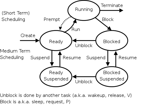
For now we are discussing the arcs connecting running↔ready in the diagram on the right showing the various states of a process. Medium term scheduling is discussed later as is disk-arm scheduling.

Naturally, the part of the OS responsible for (short-term, processor) scheduling is called the (short-term, processor) scheduler and the algorithm used is called the (short-term, processor) scheduling algorithm.

2.4.1 Introduction to Scheduling

Importance of Scheduling for Various Generations and Circumstances

Early computer systems were monoprogrammed and, as a result, scheduling was a non-issue.

For many current personal computers, which are definitely multiprogrammed, there is in fact very rarely more than one runnable process. As a result, scheduling is not critical.

For servers (or old mainframes), scheduling is indeed important and these are the systems you should think of.

Process Behavior

Processes alternate CPU bursts with I/O activity, as we shall see in lab2. The key distinguishing factor between compute-bound (aka CPU-bound) and I/O-bound jobs is the length of the CPU bursts.

The trend over the past decade or two has been for more and more jobs to become I/O-bound since the CPU rates have increased faster than the I/O rates.

When to Schedule

An obvious point, which is often forgotten (I don't think 3e mentions it) is that the scheduler cannot run when the OS is not running. In particular, for the uniprocessor systems we are considering, no scheduling can occur when a user process is running. (In the mulitprocessor situation, no scheduling can occur when all processors are running user jobs).

Again we refer to the state transition diagram above.

1. Process creation.
   The running process has issued a fork() system call and hence the OS runs; thus scheduling is possible. Scheduling is also desirable at this time since the scheduling algorithm might favor the new process.
2. Process termination.
   The exit() system call has again transferred control to the OS so scheduling is possible. It is necessary since the previously running process has terminated.
3. Process blocks.
   Same as termination.
4. Interrupt received.
   Since the OS takes control, scheduling is possible. When an I/O interrupt occurs, this normally means that a blocked process is now ready and, with a new candidate for running, scheduling is desirable.
5. Clock interrupts are treated next when we discuss preemption and discuss the dotted arc in the process state diagram.

Preemption

It is important to distinguish preemptive from non-preemptive scheduling algorithms.

• Preemption means the operating system moves a process from running to ready without the process requesting it.
• Without preemption, the system implements run until completion, yield, or block.
• The preempt arc in the diagram is present for preemptive scheduling algorithms.
• We do not emphasize yield (a solid arrow from running to ready).
• Preemption needs a clock interrupt (or equivalent).
• Preemption is needed to guarantee fairness.
• Preemption is found in all modern general purpose operating systems.
• Even non-preemptive systems can be multiprogrammed (remember that processes do block for I/O).
• Preemption is not cheap.

Categories of Scheduling Algorithms

We distinguish three categories with regard to the importance of preemption.

1. Batch.
2. Interactive.
3. Real Time.

For multiprogramed batch systems (we don't consider uniprogrammed systems, which don't need schedulers) the primary concern is efficiency. Since no user is waiting at a terminal, preemption is not crucial and if it is used, each process is given a long time period before being preempted.

For interactive systems (and multiuser servers), preemption is crucial for fairness and rapid response time to short requests.

We don't study real time systems in this course, but can say that preemption is typically not important since all the processes are cooperating and are programmed to do their task in a prescribed time window.

Scheduling Algorithm Goals

There are numerous objectives, several of which conflict, that a scheduler tries to achieve. These include.

1. Fairness.
   Treating users fairly, which must be balanced against ...
   
   
2. Respecting priority.
   That is, giving more important processes higher priority. For example, if my laptop is trying to fold proteins in the background, I don't want that activity to appreciably slow down my compiles and especially don't want it to make my system seem sluggish when I am modifying these class notes. In general, interactive jobs should have higher priority.
   
   
3. Efficiency.
   This has two aspects.
   • Do not spend excessive time in the scheduler.
   • Try to keep all parts of the system busy.
   
   
4. Low turnaround time
   That is, minimize the time from the submission of a job to its termination. This is important for batch jobs.
   
   
5. High throughput.
   That is, maximize the number of jobs completed per day. Not quite the same as minimizing the (average) turnaround time as we shall see when we discuss shortest job first.
   
   
6. Low response time.
   That is, minimize the time from when an interactive user issues a command to when the response is given. This is very important for interactive jobs.
   
   
7. Repeatability. Dartmouth (DTSS) wasted cycles and limited logins for repeatability.
   
   
8. Degrade gracefully under load.

The Name Game

There is an amazing inconsistency in naming the different (short-term) scheduling algorithms. Over the years I have used primarily 4 books: In chronological order they are Finkel, Deitel, Silberschatz, and Tanenbaum. The table just below illustrates the name game for these four books. After the table we discuss several scheduling policy in some detail.

    Finkel  Deitel  Silbershatz Tanenbaum
    -------------------------------------
    FCFS    FIFO    FCFS        FCFS
    RR      RR      RR          RR
    PS      **      PS          PS
    SRR     **      SRR         **    not in tanenbaum
    SPN     SJF     SJF         SJF
    PSPN    SRT     PSJF/SRTF   SRTF
    HPRN    HRN     **          **    not in tanenbaum
    **      **      MLQ         **    only in silbershatz
    FB      MLFQ    MLFQ        MQ
  

Remark: For an alternate organization of the scheduling algorithms (due to Eric Freudenthal and presented by him Fall 2002) click here.

2.4.2 Scheduling in Batch Systems

First Come First Served (FCFS, FIFO, FCFS, --)

If the OS doesn't schedule, it still needs to store the list of ready processes in some manner. If it is a queue you get FCFS. If it is a stack (strange), you get LCFS. Perhaps you could get some sort of random policy as well.

• Only FCFS is considered.
• Non-preemptive.
• The simplist scheduling policy.
• In some sense the fairest since it is first come first served. But perhaps that is not so fair. Consider a 1 hour job submitted one second before a 3 second job.
• The most efficient usage of cpu since the scheduler is very fast.
• Does not favor interactive jobs.

Shortest Job First (SPN, SJF, SJF, SJF)

Sort jobs by execution time needed and run the shortest first.

This is a Non-preemptive algorithm.

First consider a static situation where all jobs are available in the beginning and we know how long each one takes to run. For simplicity lets consider run-to-completion, also called uniprogrammed (i.e., we don't even switch to another process on I/O). In this situation, uniprogrammed SJF has the shortest average waiting time.

• Assume you have a schedule with a long job right before a short job.
• Consider swapping the two jobs.
• This decreases the wait for the short by the length of the long job and increases the wait of the long job by the length of the short job.
• This decreases the total waiting time for these two.
• Hence decreases the total waiting for all jobs and hence decreases the average waiting time as well.
• Hence, whenever a long job is right before a short job, we can swap them and decrease the average waiting time.
• Thus the lowest average waiting time occurs when there are no short jobs right before long jobs.
• This is uniprogrammed SJF.

The above argument illustrates an advantage of favoring short jobs (e.g., RR with small quantum): The average waiting time is reduced.

In the more realistic case of true SJF where the scheduler switches to a new process when the currently running process blocks (say for I/O), we could also consider the policy shortest next-CPU-burst first.

The difficulty is predicting the future (i.e., knowing in advance the time required for the job or the job's next-CPU-burst).

SJF Can starve a process that requires a long burst.

• This is fixed by the standard technique.
• What is that technique?
  Ans: Priority aging (see below).

Shortest Remaining Time Next (PSPN, SRT, PSJF/SRTF, SRTF)

Preemptive version of above. Indeed some authors call it preemptive shortest job first.

• Permit a process that enters the ready list to preempt the running process if the time for the new process (or for its next burst) is less than the remaining time for the running process (or for its current burst).
• It will never happen that a process already in the ready list will require less time than the remaining time for the currently running process. Why?
  Ans: When the process joined the ready list it would have started running if the current process had more time remaining. Since that didn't happen the currently running job had less time remaining and now it has even less.
• PSPN Can starve a process that requires a long burst.
  • This is fixed by the standard technique.
  • What is that technique?
    Ans: Priority aging (see below).

2.4.3 Scheduling in Interactive Systems

The following algorithms can also be used for batch systems, but in that case, the gain may not justify the extra complexity.

Round Robin (RR, RR, RR, RR)

• An important preemptive policy.
• Essentially the preemptive version of FCFS.
• The key parameter is the quantum size q.
• When a process is put into the running state a timer is set to q.
• If the timer goes off and the process is still running, the OS preempts the process.
  • This process is moved to the ready state (the preempt arc in the diagram), where it is placed at the rear of the ready list.
  • The process at the front of the ready list is removed from the ready list and run (i.e., moves to state running).
  • Note that the ready list is being treated as a queue. Indeed it is sometimes called the ready queue, but not by me since for other scheduling algorithms it is not accessed in a FIFO manner.
• When a process is created, it is placed at the rear of the ready list.
• Note that RR works well if you have a 1 hr job and then a 3 second job.
• As q gets large, RR approaches FCFS. Indeed if q is larger that the longest time any process will run before terminating or blocking, then RR IS FCFS. A good way to see this is to look at my favorite diagram and note the three arcs leaving running. They are triggered by three conditions: process terminating, process blocking, and process preempted. If the first trigger condition to arise is never preemption, we can erase that arc and then RR becomes FCFS.
• As q gets small, RR approaches PS (Processor Sharing, described next).
• What value of q should we choose?
  • Trade-off
  • Small q makes system more responsive, a long compute-bound job cannot starve a short job.
  • Large q makes system more efficient since there is less process switching.
  • A reasonable time for q is a few tens of milliseconds (millisecond = 1/1000 second and is abbreviated ms). This means every other job can delay your job by at most q (plus the context switch time CS, which is often less than 1ms). Also the overhead is CS/(CS+q), which is small.
• A student found the following reference for the name Round Robin. A similar, but less detailed, citation can be found in wikipedia.

  The round robin was originally a petition, its signatures arranged in a circular form to disguise the order of signing. Most probably it takes its name from the ruban rond, (round ribbon), in 17th-century France, where government officials devised a method of signing their petitions of grievances on ribbons that were attached to the documents in a circular form. In that way no signer could be accused of signing the document first and risk having his head chopped off for instigating trouble. Ruban rond later became round robin in English and the custom continued in the British navy, where petitions of grievances were signed as if the signatures were spokes of a wheel radiating from its hub. Today round robin usually means a sports tournament where all of the contestants play each other at least once and losing a match doesn't result in immediate elimination.
  
  Encyclopedia of Word and Phrase Origins by Robert Hendrickson (Facts on File, New York, 1997).

Homework: 20, 35.

Homework: Round-robin schedulers normally maintain a list of all runnable processes, with each process occurring exactly once in the list. What would happen if a process occurred more than once in the list? Can you think of any reason for allowing this?

Homework: Give an argument favoring a large quantum; give an argument favoring a small quantum.

Process	CPU Time	Creation Time
P1	20	0
P2	3	3
P3	2	5

Homework:

• Consider the set of processes in the table to the right.
• When does each process finish if RR scheduling is used with q=1, if q=2, if q=3, if q=100?
• First assume (unrealistically) that context switch time is zero.
• Then assume it is .1. Each process performs no I/O (i.e., no process ever blocks).
• All times are in milliseconds.
• The CPU time is the total time required for the process (excluding any context switch time).
• The creation time is the time when the process is created. So P1 is created when the problem begins and P3 is created 5 milliseconds later.
• If two processes have equal priority (in RR this means if thy both enter the ready state at the same cycle), we give priority (in RR this means place first on the queue) to the process with the earliest creation time. If they also have the same creation time, then we give priority to the process with the lower number.
• Remind me to discuss this last one in class next time.

Homework: Redo the previous homework for q=2 with the following change. After process P1 runs for 3ms (milliseconds), it blocks for 2ms. P1 never blocks again. P2 never blocks. After P3 runs for 1 ms it blocks for 1ms. Remind me to answer this one in class next lecture.

Processor Sharing (PS, **, PS, PS)

Merge the ready and running states and permit all ready jobs to be run at once. However, the processor slows down so that when n jobs are running at once, each progresses at a speed 1/n as fast as it would if it were running alone.

• Clearly impossible as stated due to the overhead of process switching.
• Of theoretical interest (easy to analyze).
• Approximated by RR when the quantum is small. Make sure you understand this last point. For example, consider the last homework assignment (with zero context switch time and no blocking) and consider q=1, q=.1, q=.01, etc.
• Show what happens for 3 processes, A, B, C, each requiring 3 seconds of CPU time. A starts at time 0, B at 1 second, C at 2.
• Consider three processes all starting at time 0. One requires 1ms, the second 100ms, the third 10sec (seconds). Compute the total/average waiting time for RR q=1ms, PS, SJF, SRTN, and FCFS. Note that this depends on the order the processes happen to be processed in. The effect is huge for FCFS, modest for RR with modest quantum, and non-existent for PS and SRTN.

Homework: 32.

Variants of Round Robin

1. State dependent RR
   • Same as RR but q is varied dynamically depending on the state of the system.
   • Favor processes holding important resources, for example, non-swappable memory.
   • Perhaps this should be considered medium term scheduling since you probably do not recalculate q each time.
2. External priorities: RR but a user can pay more and get bigger q. That is, one process can be given a higher priority than another. But this is not an absolute priority: the lower priority (i.e., less important) process does get to run, but not as much as the higher priority process.

Priority Scheduling

Each job is assigned a priority (externally, perhaps by charging more for higher priority) and the highest priority ready job is run.

• Similar to External priorities above
• If many processes have the highest priority, use RR among them. Indeed one often groups several priorities into a priority class and employs RR within a class.
• Can easily starve processes (see aging below for fix).
• Can have the priorities changed dynamically to favor processes holding important resources (similar to state dependent RR).
• Many policies can be thought of as priority scheduling in which we run the job with the highest priority. The different scheduling policies have different notions of priority. For example:
  • FCFS and RR are priority scheduling where the priority is the time spent on the ready list.
  • SJF and SRTN are priority scheduling, where the priority of the job is the negative of the time it needs to run in order to complete (or complete its current CPU burst).

Priority aging

As a job is waiting, raise its priority so eventually it will have the maximum priority.

• This prevents starvation (assuming all jobs terminate or the policy is preemptive).
• Starvation means that some process is never run, because it never has the highest priority. It is also starvation, if process A runs for a while, but then is never able to run again, even though it is ready. The formal way to say this is No job can remain in the ready state forever.
• There may be many processes with the maximum priority.
• If so, can use FIFO among those with max priority (risks starvation if a job doesn't terminate) or can use RR.
• Can apply priority aging to many policies, in particular to priority scheduling described above.

Homework: 36, 37. Note that when the book says RR with each process getting its fair share, it means Processor Sharing.

Selfish RR (SRR, **, SRR, **)

SRR is a preemptive policy in which unblocked (i.e. ready and running) processes are divided into two classes the Accepted processes, which run RR and the others (perhaps SRR really stands for snobbish RR).

• Accepted process have their priority increase at rate a≥0.
• A new process starts at priority 0; its priority increases at rate b≥0.
• An unaccepted process becomes an accepted process when its priority reaches that of the accepted processes (or when there are no accepted processes).
• Hence, once a process is accepted, it remains accepted until it terminates (or blocks, see below) and all accepted processes have same priority.
• Note that, when the only accepted process terminates (or blocks, see below), all the process with the next highest priority become accepted.

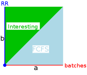
The behavior of SRR depends on the relationship between a and b (and zero).

• If a=0, get RR.
• If a≥b>0, get FCFS.
• If b>a>0, it is interesting.
• If a>b=0, you get RR in batches. This is similar to n-step scan for disk I/O.

It is not clear what is supposed to happen when a process blocks. Should its priority get reset to zero and have unblock act like create? Should the priority continue to grow (at rate a or b)? Should its priority be frozen during the blockage. Let us assume the first case (reset to zero) since it seems the simplest.

Remark: Recall that SFJ/PSFJ do a good job of minimizing the average waiting time. The problem with them is the difficulty in finding the job whose next CPU burst is minimal. We now learn three scheduling algorithms that attempt to do this. The first algorithm does it statically, presumably with some manual help; the other two are dynamic and fully automatic.

Multilevel Queues (**, **, MLQ, **)

Put different classes of processs in different queues

• Processes do not move from one queue to another.
• Can have different policies on the different queues.
  For example, might have a background (batch) queue that is FCFS and one or more foreground queues that are RR (possibly with different quanta).
• Must also have a policy among the queues.
  For example, might have two queues, foreground and background, and give the first absolute priority over the second
  • Might apply priority aging to prevent background starvation.
  • But might not, i.e., no guarantee of service for background processes. View a background process as a cycle soaker.
  • Might have 3 queues, foreground, background, cycle soaker.

Multiple Queues (FB, MFQ, MLFBQ, MQ)

As with multilevel queues above we have many queues, but now processes move from queue to queue in an attempt to dynamically separate batch-like from interactive processs so that we can favor the latter.

• Remember that average waiting time is achieved by SJF and this is an attempt to determine dynamically those processes that are interactive, which means have a very short cpu burst.
• Run processs from the highest priority nonempty queue in a RR manner.
• When a process uses its full quanta (looks a like batch process), move it to a lower priority queue.
• When a process doesn't use a full quanta (looks like an interactive process), move it to a higher priority queue.
• A long process with frequent (perhaps spurious) I/O will remain in the upper queues.
• Might have the bottom queue FCFS.
• Many variants.
  For example, might let process stay in top queue 1 quantum, next queue 2 quanta, next queue 4 quanta (i.e., sometimes return a process to the rear of the same queue it was in if the quantum expires).
  Might move to a higher queue only if a keyboard interrupt occurred rather than if the quantum failed to expire for any reason (disk I/O).

Shortest Process Next

An attempt to apply sjf to interactive scheduling. What is needed is an estimate of how long the process will run until it blocks again. One method is to choose some initial estimate when the process starts and then, whenever the process blocks choose a new estimate via

    NewEstimate = A*OldEstimate + (1-A)*LastBurst
  

Highest Penalty Ratio Next (HPRN, HRN, **, **)

Run the process that has been hurt the most.

• For each process, let r = T/t; where T is the wall clock time this process has been in system and t is the running time of the process to date.
• If r=2.5, that means the job has been running 1/2.5 = 40% of the time it has been in the system.
• We call r the penalty ratio and run the process having the highest r value.
• We must worry about a process that just enters the system since t=0 and hence the ratio is undefined. Define t to be the max of 1 and the running time to date. Since now t is at least 1, the ratio is always defined.
• HPRN is normally defined to be non-preemptive (i.e., the system only checks r when a burst ends), but there is an preemptive analogue
  • When putting a process into the run state compute the time at which it will no longer have the highest ratio and set a timer.
  • When a process is moved into the ready state, compute its ratio and preempt if needed.
• HRN stands for highest response ratio next and means the same thing.
• This policy is yet another example of priority scheduling

Guaranteed Scheduling

A variation on HPRN. The penalty ratio is a little different. It is nearly the reciprocal of the above, namely
   t / (T/n)
where n is the multiprogramming level. So if n is constant, this ratio is a constant times 1/r.

Lottery Scheduling

Each process gets a fixed number of tickets and at each scheduling event a random ticket is drawn (with replacement) and the process holding that ticket runs for the next interval (probably a RR-like quantum q).

On the average a process with P percent of the tickets will get P percent of the CPU (assuming no blocking, i.e., full quanta).

Fair-Share Scheduling

If you treat processes fairly you may not be treating users fairly since users with many processes will get more service than users with few processes. The scheduler can group processes by user and only give one of a user's processes a time slice before moving to another user.

Fancier methods have been implemented that give some fairness to groups of users. Say one group paid 30% of the cost of the computer. That group would be entitled to 30% of the cpu cycles providing it had at least one process active. Furthermore a group earns some credit when it has no processes active.

Theoretical Issues

Considerable theory has been developed.

• NP completeness results abound.
• Much work in queuing theory to predict performance.
• Not covered in this course.

Medium-Term Scheduling

In addition to the short-term scheduling we have discussed, we add medium-term scheduling in which decisions are made at a coarser time scale.

Suspend (swap out) some process if memory is over-committed. Suspend gives rise to the arcs in the process state diagram leading down to the suspended states we haven't yet discussed.

Criteria for choosing a victim.

• How long since previously suspended.
• How much CPU time used recently.
• How much memory does it use.
• External priority (pay more, get swapped out less).

We will discuss medium term scheduling again when we study memory management.

Long Term Scheduling

This is sometimes called Job scheduling.

1. The system decides when to start jobs, i.e., it does not necessarily start them when submitted.
2. Used at many supercomputer sites.

A similar idea (but more drastic and not always so well coordinated) is to force some users to log out, kill processes, and/or block logins if over-committed.

• CTSS (an early time sharing system at MIT) did this to insure decent interactive response time.
• Unix does this if out of memory.
• LEM jobs during the day (Grumman).

2.7 Summary

Skipped, but you should read.

Lecture #5 Resumes

Chapter 6 Deadlocks

Remark: Deadlocks are closely related to process management so belong here, right after chapter 2. It was here in 2e. A goal of 3e is to make sure that the basic material gets covered in one semester. But I know we will do the first 6 chapters so there is no need for us to postpone the study of deadlock.

A deadlock occurs when every member of a set of processes is waiting for an event that can only be caused by a member of the set.

Often the event waited for is the release of a resource.

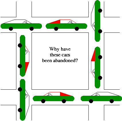
In the automotive world deadlocks are called gridlocks.

• The processes are the cars.
• The resources are the spaces occupied by the cars

For a computer science example consider two processes A and B that each want to print a file currently on a CD-ROM Drive.

1. A has obtained ownership of the printer and will release it after getting the CD Drive and printing one file.
2. B has obtained ownership of the CD drive and will release it after getting the printer and printing one file.
3. A tries to get ownership of the drive, but is told to wait for B to release it.
4. B tries to get ownership of the printer, but is told to wait for A to release it.

Bingo: deadlock!

6.1 Resources

A resource is an object granted to a process.

6.1.1 Preemptable and Nonpreemptable Resources

Resources come in two types

1. Preemptable, meaning that the resource can be taken away from its current owner (and given back later). An example is memory.
2. Non-preemptable, meaning that the resource cannot be taken away. An example is a printer.

The interesting issues arise with non-preemptable resources so those are the ones we study.

The life history of a resource is a sequence of

1. Request
2. Allocate
3. Use
4. Release

Processes request the resource, use the resource, and release the resource. The allocate decisions are made by the system and we will study policies used to make these decisions.

6.1.2 Resource Acquisition

A simple example of the trouble you can get into.

• Two resources and two processes.
• Each process wants both resources.
• Use a semaphore for each. Call them S and T.
• If both processes execute
  P(S); P(T); --- V(T); V(S)
  all is well.
• But if one executes instead
  P(T); P(S); -- V(S); V(T)
  disaster! This was the printer/CD example just above.

Recall from the semaphore/critical-section treatment last chapter, that it is easy to cause trouble if a process dies or stays forever inside its critical section. We assume processes do not do this. Similarly, we assume that no process retains a resource forever. It may obtain the resource an unbounded number of times (i.e. it can have a loop forever with a resource request inside), but each time it gets the resource, it must release it eventually.

6.2 Introduction to Deadlocks

Definition: A deadlock occurs when a every member of a set of processes is waiting for an event that can only be caused by a member of the set.

Often the event waited for is the release of a resource.

Note on lab 2 (scheduling).
If several processes are waiting on I/O, you are to assume noninterference. For example, assume that on cycle 100 process A flips a coin and decides its wait is 6 units (i.e., during cycles 101-106 A will be blocked. Assume B begins running at cycle 101 for a burst of 1 cycle. After this cycle process B flips a coin and decides its wait is 3 units. You do NOT alter process A. That is, Process A will become ready after cycle 106 (100+6) so enters the ready list cycle 107 and process B becomes ready after cycle 104 (101+3) and enters ready list cycle 105.
End of Note

6.2.1 (Necessary) Conditions for Deadlock

The following four conditions (Coffman; Havender) are necessary but not sufficient for deadlock. Repeat: They are not sufficient.

1. Mutual exclusion: A resource can be assigned to at most one process at a time (no sharing).
2. Hold and wait: A processing holding a resource is permitted to request another.
3. No preemption: A process must release its resources; they cannot be taken away.
4. Circular wait: There must be a chain of processes such that each member of the chain is waiting for a resource held by the next member of the chain.

One can say If you want a deadlock, you must have these four conditions.. But of course you don't actually want a deadlock, so you would more likely say If you want to prevent deadlock, you need only violate one or more of these four conditions..

The first three are static characteristics of the system and resources. That is, for a given system with a fixed set of resources, the first three conditions are either always true or always false: They don't change with time. The truth or falsehood of the last condition does indeed change with time as the resources are requested/allocated/released.

6.2.2 Deadlock Modeling

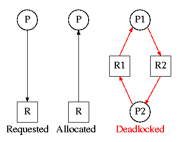
On the right are several examples of a Resource Allocation Graph, also called a Reusable Resource Graph.

• The processes are circles.
• The resources are squares.
• An arc (directed line) from a process P to a resource R signifies that process P has requested (but not yet been allocated) resource R.
• An arc from a resource R to a process P indicates that process P has been allocated resource R.

Homework: 5.

Consider two concurrent processes P1 and P2 whose programs are.

    P1                   P2
    request R1           request R2
    request R2           request R1
    release R2           release R1
    release R1           release R2
  

On the board draw the resource allocation graph for various possible executions of the processes, indicating when deadlock occurs and when deadlock is no longer avoidable.

There are four strategies used for dealing with deadlocks.

1. Ignore the problem
2. Detect deadlocks and recover from them
3. Prevent deadlocks by violating one of the 4 necessary conditions.
4. Avoid deadlocks by carefully deciding when to allocate resources.