Start Lecture #14
We now need to access the ARs from the stack. The key distinction is that the location of the current AR is not known at compile time. Instead a pointer to the stack must be maintained dynamically.
We dedicate a register, call it SP, for this purpose.
In this chapter we let SP point to the bottom of the current AR,
that is the entire AR is above the SP.
Since we are not supporting varargs, there is no advantage to having
SP point to the middle
of the AR as in the previous chapter.
The main procedure (or the run-time library code called before
any user-written procedure) must initialize SP with
LD SP, #stackStart
where stackStart is a known-at-compile-time constant.
The caller increments SP (which now points to the beginning of its AR) to point to the beginning of the callee's AR. This requires an increment by the size of the caller's AR, which of course the caller knows.
Is this size a compile-time constant?
The book treats it as a constant. The only part that is not known at compile time is the size of the dynamic arrays. Strictly speaking this is not part of the AR, but it must be skipped over since the callee's AR starts after the caller's dynamic arrays.
Perhaps for simplicity we are assuming that there are no dynamic arrays being stored on the stack. If there are arrays, their size must be included in some way.
The code generated for a parameterless call is
    ADD SP, SP, #caller.ARSize
    ST  0(SP), #here+16        // save return address (book wrong)
    BR  callee.codeArea
The return requires code from both the Caller and Callee.
The callee transfers control back to the caller with
BR *0(SP)
Upon return the caller restore the stack pointer with
SUB SP, SP, #caller.ARSize
We again consider a main program calling a procedure P and then halting. Other actions by Main and P are indicated by subscripted uses of `other'.
    // Quadruples of Main
    other1
    call P
    other2
    halt
    // Quadruples of P
    other3
    return
Recall our assumptions that the code for Main starts in location 1000, the code for P starts in location 2000, and each otheri requires 100 bytes. Let us assume the stack begins at 9000 (and grows to larger addresses) and that the AR for Main is of size 400 (we don't need P.ARSize since P doesn't call any procedures). Then the following machine code results.
    // Code for Main
    1000: LD  SP, 9000        // Possibly done prior to Main
    1008: Other1
    1108: ADD SP, SP, #400
    1116: ST  0(SP), #1132    // Understand the address
    1124: BR, 2000
    1132: SUB SP, SP, #400
    1140: other2
    1240: HALT
    ...
    // Code for P
    2000: other3
    2100: BR *0(SP)           // Understand the *
    ...
    // AR for Main
    9000:                     // Return address stored here (not used)
    9004:                     // Local data for Main starts here
    9396:                     // Last word of the AR is bytes 9396-9399
    ...
    // AR for P
    9400:                     // Return address stored here
    9404:                     // Local data for P starts here
    9496:                     // Last word of the AR is bytes 9496-9799
Homework: 1, 2, 3.
A technical fine point about static allocation and a corresponding point about the display.
As we have seen, for many quads it is quite easy to generate a series of machine instructions to achieve the same effect. As we have also seen, the resulting code can be quite inefficient. For one thing the last instruction generated for a quad is often a store of a value that is then loaded right back in the next quad (or one or two quads later).
Another problem is that we don't make much use of the registers. That is, translating a single quad needs just one or two registers so we might as well throw out all the other registers on the machine.
Both of the problems are due to the same cause: Our horizon is too limited. We must consider more than one quad at a time. But wild flow of control can make it unclear which quads are dynamically near each other. So we want to consider, at one time, a group of quads for which the dynamic order of execution is tightly controlled. We then also need to understand how execution proceeds from one group to another. Specifically the groups are called basic blocks and the execution order among them is captured by the flow graph.
Definition: A basic block is a maximal collection of consecutive quads such that
Definition: A flow graph has the basic blocks as vertices and has edges from one block to each possible dynamic successor.
We process all the quads in a basic block together
making
use of the fact that the block is not entered or left in
the middle
.
Constructing the basic blocks is easy. Once you find the start of a block, you keep going until you hit a label or jump. But, as usual, to say it correctly takes more words.
Definition: A basic block leader (i.e., first instruction) is any of the following (except for the instruction just past the entire program).
Given the leaders, a basic block starts with a leader and proceeds up to but not including the next leader.
The following code produces a 10x10 real identity matrix
    for i from 1 to 10 do
      for j from 1 to 10 do
        a[i,j] = 0
      end
    end
    for i from 1 to 10 do
      a[i,i] = 1.0
    end
The following quads do the same thing. Don't worry too much about how the quads were generated.
     1)  i = 1
     2)  j = 1
     3)  t1 = 10 * i
     4)  t2 = t1 + j        // element [i,j]
     5)  t3 = 8 * t2        // offset for a[i,j] (8 byte reals)
     6)  t4 = t3 - 88       // program array starts at [1,1] assembler at [0,0]
     7)  a[t4] = 0.0
     8)  j = j + 1
     9)  if j <= 10 goto (3)
    10)  i = i + 1
    11)  if i <= 10 goto (2)
    12)  i = 1
    13)  t5 = i - 1
    14)  t6 = 88 * t5
    15)  a[t6] = 1.0
    16)  i = i + 1
    17)  if i <= 10 goto (13)
Which quads are leaders?
1 is a leader by definition. The jumps are 9, 11, and 17. So 10 and 12 are leaders as are the targets 3, 2, and 13.
The leaders are then 1, 2, 3, 10, 12, and 13.
The basic blocks are therefore {1}, {2}, {3,4,5,6,7,8,9}, {10,11}, {12}, and {13,14,15,16,17}.
Here is the code written again with the basic blocks indicated.
     1)  i = 1

     2)  j = 1

     3)  t1 = 10 * i
     4)  t2 = t1 + j            // element [i,j]
     5)  t3 = 8 * t2            // offset for a[i,j] (8 byte numbers)
     6)  t4 = t3 - 88           // we start at [1,1] not [0,0]
     7)  a[t4] = 0.0
     8)  j = j + 1
     9)  if J <= 10 goto (3)

    10)  i = i + 1
    11)  if i <= 10 goto (2)

    12)  i = 1

    13)  t5 = i - 1
    14)  t6 = 88 * t5
    15)  a[t6] = 1.0
    16)  i = i + 1
    17)  if i <= 10 goto (13)
We can see that once you execute the leader you are assured of executing the rest of the block in order.
We want to record the flow of information from instructions that compute a value to those that use the value. One advantage we will achieve is that if we find a value has no subsequent uses, then it is dead and the register holding that value can be used for another value.
Assume that a quad p assigns a value to x (some would call this a def of x).
Definition: A quad q uses the value computed at p (uses the def) and x is live at q if q has x as an operand and there is a possible execution path from p to q that does not pass any other def of x.
Since the flow of control is trivial inside a basic block, we are able to compute the live/dead status and next use information at the block leader by a simple backwards scan of the quads (algorithm below).
Note that if x is dead (i.e., defined before used) on entrance to B the register containing x can be reused in B.
Our goal is to determine whether a block uses a value and if so in which statement is it first used. The following algorithm for computing uses is quite simple.
    Initialize all variables in B as being live
    Examine the quads q of the block in reverse order.
        Assume the quad q computes x and reads y and z
        Mark x as dead; mark y and z as live and used at q
When the loop finishes those values that are read before being written are marked as live and their first use is noted. The locations x that are written before being read are marked dead meaning that the value of x on entrance is not used.
Those values that are neither read nor written remain simply live.
They are not dead since the dynamically next
basic block might use them.
Note that we have determined whether values are live/dead on entrance to the basic block. We would like to know as well if they are live/dead on exit, but that requires global flow analysis, which we do not know.
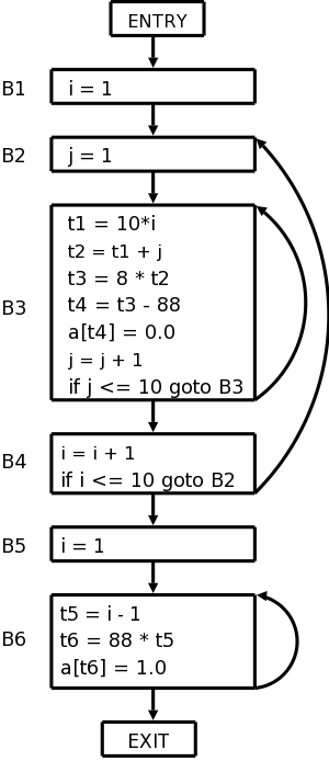
The nodes of the flow graph are the basic blocks, and there is an edge from P (predecessor) to S (successor) if S might follow P. More formally, such an edge is added if the last statement of P
Two nodes are added: entry
and exit
.
An edge is added from entry to the first basic block, i.e. the block
that has the first statement of the program as leader.
Edges to the exit are added from any block that could be the last block executed. Specifically, edges are added to exit from
The flow graph for our example is shown on the right.
Note that jump targets are no longer quads but blocks. The reason is that various optimizations within blocks will change the instructions and we would have to change the jump to reflect this.
For most programs the bulk of the execution time is within loops so we want to identify these.
The flow graph on the right has three loops.
Homework: 1.
Remark: Nothing beyond here will be on the final.
We are not covering global flow analysis; it is a key component of optimization and would be a natural topic in a follow-on course. Nonetheless there is something we can say just by examining the flow graphs we have constructed. For this discussion I am ignoring tricky and important issues concerning arrays and pointer references (specifically, disambiguation). You may wish to assume that the program contains no arrays or pointers.
We have seen that a simple backwards scan of the statements in a
basic block enables us to determine the variables that are
live-on-entry and those that are dead-on-entry.
Those variables that do not occur in the block are in neither
category; perhaps we should call them ignored by the block
.
We shall see below that it would be lovely to know which variables are live/dead-on-exit. This means which variables hold values at the end of the block that will / will not be used. To determine the status of v on exit of a block B, we need to trace all possible execution paths beginning at the end of B. If all these paths reach a block where v is dead-on-entry before they reach a block where v is live-on-entry, then v is dead on exit for block B.
The goal is to obtain a visual picture of how information flows through the block. The leaves will show the values entering the block and as we proceed up the DAG we encounter uses of these values, defs (and redefs) of values, and uses of the new values.

Formally, this is defined as follows.
live on exit, an officially-mysterious term meaning values possibly used in another block. (Determining the live on exit values requires global, i.e., inter-block, flow analysis.)
As we shall see in the next few sections various basic-block optimizations are facilitated by using the DAG.
As we create nodes for each statement, proceeding in the static order of the statements, we might notice that a new node is just like one already in the DAG in which case we don't need a new node and can use the old node to compute the new value in addition to the one it already was computing.
Specifically, we do not construct a new node if an existing node has the same children in the same order and is labeled with the same operation.
Consider computing the DAG for the following block of code.
    a = b + c
    c = a + x
    d = b + c
    b = a + x
The DAG construction proceeds as follows (the movie on the right accompanies the explanation).
You might think that with only three computation nodes in the DAG,
the block could be reduced to three statements (dropping the
computation of b).
However, this is wrong.
Only if b is dead on exit can we omit the computation of b.
We can, however, replace the last statement with the simpler
b = c.
Sometimes a combination of techniques finds improvements that no single technique would find. For example if a-b is computed, then both a and b are incremented by one, and then a-b is computed again, it will not be recognized as a common subexpression even though the value has not changed. However, when combined with various algebraic transformations, the common value can be recognized.
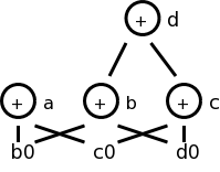
Assume we are told (by global flow analysis) that certain values are dead on exit. We examine each root (node with no ancestor) and delete any for which all attached variables are dead on exit. This process is repeated since new roots may have appeared.
For example, if we are told, for the picture on the right, that c and d are dead on exit, then the root d can be removed since d is dead. Then the rightmost node becomes a root, which also can be removed (since c is dead).
Some of these are quite clear. We can of course replace x+0 or 0+x by simply x. Similar considerations apply to 1*x, x*1, x-0, and x/1.
Another class of simplifications is strength reduction, where we replace one operation by a cheaper one. A simple example is replacing 2*x by x+x on architectures where addition is cheaper than multiplication.
A more sophisticated strength reduction is applied by compilers that
recognize induction variables
(loop indices).
Inside a
for i from 1 to N
loop, the expression 4*i can be strength reduced to j=j+4 and 2^i
can be strength reduced to j=2*j (with suitable initializations of j
just before the loop).
Other uses of algebraic identities are possible; many require a
careful reading of the language reference manual to ensure their
legality.
For example, even though it might be advantageous to convert
((a + b) * f(x)) * a
to
((a + b) * a) * f(x)
it is illegal in Fortran since the programmer's use of parentheses
to specify the order of operations can not be violated.
Does
    a = b + c
    x = y + c + b + r
contain a common subexpression of b+c that need be evaluated only
once?Arrays are tricky. Question: Does
    x = a[i]
    a[j] = y
    z = a[i]
contain a common subexpression of a[i] that need be evaluated only
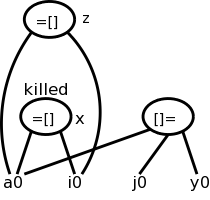
once?A statement of the form x = a[i] generates a node labeled with the operator =[] and the variable x, and having children a0, the initial value of a, and the value of i.

A statement of the form a[j] = y generates a node labeled with operator []= and three children a0. j, and y, but with no variable as label. The new feature is that this node kills all existing nodes depending on a0. A killed node can not received any future labels so cannot becomew a common subexpression.
Returning to our example
    x = a[i]
    a[j] = y
    z = a[i]
We obtain the top figure to the right.
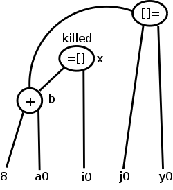
Sometimes it is not children but grandchildren (or other descendant) that are arrays. For example we might have
    b = a + 8    // b[i] is 8 bytes past a[i]
    x = b[i]
    b[j] = y
We are using C-like semantics, where an array references is thought
to be a pointer to a[0], the first element of the array.
Hence b is a pointer to 8 bytes past the first element of a, which
is a[2] for an integer array and a[1] for a real array.
Again we need to have the third statement kill the second node even
though the actual array (a) is a grandchild.
This is shown in the bottom figure.
Pointers are even trickier than arrays.
Together they have spawned a mini-industry in disambiguation
,
i.e., when can we tell whether two array or pointer references refer
to the same or different locations.
A trivial case of disambiguation occurs with.
    p = &x
    *p = y
In this case we know precisely the value of p so the second
statement kills only nodes with x attached.
With no disambiguation information, we must assume that a pointer can refer to any location. Consider
    x = *p
    *q = y
We must treat the first statement as a use of every variable; pictorially the =* operator takes all current nodes with identifiers as arguments. This impacts dead code elimination.
We must treat the second statement as writing every variable. That is all existing nodes are killed, which impacts common subexpression elimination.
In our basic-block level approach, a procedure call has properties similar to a pointer reference: For all x in the scope of P, we must treat a call of P as using all nodes with x attached and also killing those same nodes.
Now that we have improved the DAG for a basic block, we need to regenerate the quads. That is, we need to obtain the sequence of quads corresponding to the new DAG.
We need to construct a quad for every node that has a variable attached. If there are several variables attached we chose a live-on-exit variable, assuming we have done the necessary global flow analysis to determine such variables).
If there are several live-on-exit variables we need to compute one and make a copy so that we have both. An optimization pass may eliminate the copy if it is able to assure that one such variable may be used whenever the other is referenced.
Recall the example from our movie
    a = b + c
    c = a + x
    d = b + c
    b = a + x
If b is dead on exit, the first three instructions suffice. If not we produce instead
    a = b + c
    c = a + x
    d = b + c
    b = c
which is still an improvement as the copy instruction is less
expensive than the addition on most architectures.
If global analysis shows that, whenever this definition of b is used, c contains the same value, we can eliminate the copy and use c in place of b.
Note that of the following 5 rules, 2 are due to arrays, and 2 due to pointers.
Homework: 1, 2,
A big issue is proper use of the registers, which are often in short supply, and which are used/required for several purposes.
For this section we assume a RISC architecture. Specifically, we assume only loads and stores touch memory; that is, the instruction set consists of
    LD  reg, mem
    ST  mem, reg
    OP  reg, reg, reg
where there is one OP for each operation type used in the three
address code.
We will not consider the use of constants so we need not consider if
constants can be used in place of registers.
A major simplification is we assume that, for each three address operation, there is precisely one machine instruction that accomplishes the task. This eliminates the question of instruction selection.
We do, however, consider register usage. Although we have not done global flow analysis (part of optimization), we will point out places where live-on-exit information would help us make better use of the available registers.
Recall that the mem operand in the load LD and store ST instructions can use any of the previously discussed addressing modes.
These are the primary data structures used by the code generator. They keep track of what values are in each register as well as where a given value resides.
The register descriptor could be omitted since you can compute it from the address descriptors.
There are basically three parts to (this simple algorithm for) code generation.
We will isolate register allocation in a function getReg(Instruction), which is presented later. First presented is the algorithm to generate instructions. This algorithm uses getReg() and the descriptors. Then we learn how to manage the descriptors and finally we study getReg() itself.
Given a quad OP x, y, z (i.e., x = y OP z), proceed as follows.
Call getReg(OP x, y, z) to get Rx, Ry, and Rz, the registers to be used for x, y, and z respectively.
Note that getReg merely selects the registers, it does not guarantee that the desired values are present in these registers.
Check the register descriptor for Ry.
If y is not present in Ry, check the address descriptor
for y and issue
LD Ry, y'
y' is some location containing y. Perhaps y is in a register other than Ry
When processing
x = y
steps 1 and 2 are analogous to the above, step 3 is vacuous, and
step 4 is omitted since getReg() will set
Rx=Ry.
Note that if y was already in a register before the copy instruction, no code is generated at this point (getReg will choose Ry to be a register containing y). Also note that since the value of x is now not in its memory location, we may need to store this value into x at block exit.
You may have noticed that we have not yet generated any store instructions. They occur here (and during spill code in getReg()). We need to ensure that all variables needed by (dynamically) subsequent blocks (i.e., those live-on-exit) have their current values in their memory locations.
This is fairly clear. We just have to think through what happens when we do a load, a store, an (assembler) OP, or a copy. For R a register, let Desc(R) be its register descriptor. For x a program variable, let Desc(x) be its address descriptor.
Since we haven't specified getReg() yet, we will assume there are an unlimited number of registers so we do not need to generate any spill code (saving the register's value in memory). One of getReg()'s jobs is to generate spill code when a register needs to be used for another purpose and the current value is not presently in memory.
Despite having ample registers and thus not generating spill code, we will not be wasteful of registers.
This example is from the book. I give another example after presenting getReg(), that I believe justifies my claim that the book is missing an action for load instructions, as indicated above.
Assume a, b, c, and d are program variables and t, u, v are compiler generated temporaries (I would call these t$1, t$2, and t$3). The intermediate language program is in the middle with the generated code for each quad shown. To the right is shown the contents of all the descriptors. The code generation is explained on the left.
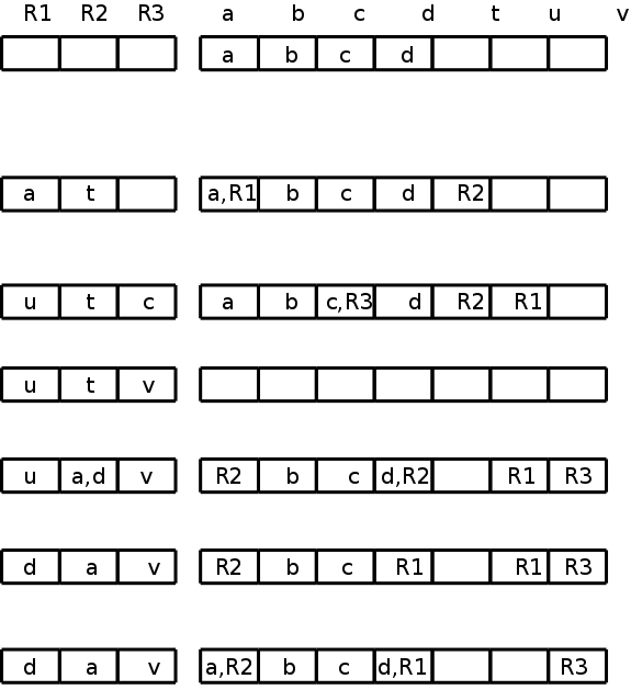
t = a - b
    LD  R1, a
    LD  R2, b
    SUB R2, R1, R2


u = a - c
    LD  r3, c
    SUB R1, R1, R3


v = t + u
    ADD R3, R2, R1


a = d
    LD  R2, d


d = v + u
    ADD R1, R3, R1


exit
    ST  a, R2
    ST  d, R1
Consider
x = y OP z
Picking registers for y and z are the same; we just do y.
Choosing a register for x is a little different.
A copy instruction
x = y
is easier.
Similar to demand paging, where the goal is to produce an available frame, our objective here is to produce an available register we can use for Ry. We apply the following steps in order until one succeeds. (Step 2 is a special case of step 3.)
As stated above choosing Rz is the same as choosing Ry.
Choosing Rx has the following differences.
getReg(x=y) chooses Ry as above and chooses Rx=Ry.
                              R1  R2  R3    a    b    c    d    e
  			                  a    b    c    d    e

    a = b + c
        LD  R1, b
        LD  R2, c
        ADD R3, R1, R2
                              R1  R2  R3    a    b    c    d    e
  			    b   c   a     R3  b,R1 c,R2  d    e

    d = a + e
        LD  R1, e
        ADD R2, R3, R1
                              R1  R2  R3    a    b    c    d    e
                       2e →   e   d   a     R3  b,R1  c    R2  e,R1
                       me →   e   d   a     R3   b    c    R2  e,R1
We needed registers for d and e; none were free. getReg() first chose R2 for d since R2's current contents, the value of c, was also located in memory. getReg() then chose R1 for e for the same reason.
Using the 2e algorithm, b might appear to be in R1 (depends if you look in the address or register descriptors).
    a = e + d
        ADD R3, R1, R2
                              Descriptors unchanged

    e = a + b
        ADD R1, R3, R1   ← possible wrong answer from 2e
                              R1  R2  R3    a    b    c    d    e
                              e   d    a    R3  b,R1  c    R2   R1

        LD  R1, b
        ADD R1, R3, R1
                              R1  R2  R3    a    b    c    d    e
                              e   d    a    R3   b    c    R2   R1
The 2e might think R1 has b (address descriptor) and also conclude R1 has only e (register descriptor) so might generate the erroneous code shown.
Really b is not in a register so must be loaded. R3 has the value of a so was already chosen for a. R2 or R1 could be chosen. If R2 was chosen, we would need to spill d (we must assume live-on-exit, since we have no global flow analysis). We choose R1 since no spill is needed: the value of e (the current occupant of R1) is also in its memory location.
  exit
      ST  a, R3
      ST  d, R2
      ST  e, R1
What if a given quad needs several OPs and we have choices?
We would like to be able to describe the machine OPs in a way that enables us to find a sequence of OPs (and LDs and STs) to do the job.
The idea is that you express the quad as a tree and express each OP
as a (sub-)tree simplification, i.e. the op replaces a subtree by a
simpler subtree.
In fact the simpler subtree is just a single node.
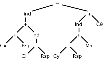
The diagram on the right represents x[i] = y[a] + 9, where x and y are on the stack and a is in the static area. M's are values in memory; C's are constants; and R's are registers. The weird ind (presumably short for indirect) treats its argument as a memory location.
Compare this to grammars: A production replaces the RHS by the LHS. We consider context free grammars where the LHS is a single nonterminal.
For example, a LD replaces a Memory node with a Register node.
Another example is that ADD Ri, Ri, Rj replaces a subtree consisting of a + with both children registers (i and j) with a Register node (i).
As you do the pattern matching and reductions (apply the productions), you emit the corresponding code (semantic actions). So to support a new processor, you need to supply the tree transformations corresponding to every instruction in the instruction set.
This is quite cute.
We assume all operators are binary and label the instruction tree with something like the height. This gives the minimum number of registers needed so that no spill code is required. A few details follow.
expression tree, the abstract syntax tree for an expression.
biggerchild all L parent regs.
Can see this is optimal (assuming you have enough registers).
Rough idea is to apply the above recursive algorithm, but at each recursive step, if the number of regs is not enough, store the result of the first child computed before starting the second.