Compilers

Start Lecture #10

Multiple Declarations in the Class Grammar

On the right we show the part of the SDD used to translate multiple declarations for the class grammar. We do not show the productions for name-and-parameters (np), statements (ss), or statement (s) since we are focusing just on the declaration of local variables.

The new part is determining the offset for each individual declaration. The new items have blue backgrounds (this includes new, inherited attributes, which were red). The idea is that the first declaration has offset 0 and the next offset is the current offset plus the current size. Specifically, we proceed as follows.

In the procedure-def (pd) production, we give the nonterminal declarations (ds) the inherited attribute offset (ds.offset), which we initialize to zero.

We inherit this offset down to individual declarations. At each declaration (d), we store the offset in the entry for the identifier being declared and increment the offset by the size of this object.

When we get the to the end of the declarations (the ε-production), the offset value is the total size needed. We turn it around and send it back up the tree in case the total is needed by some higher level production.

Example: What happens when the following program (an extension of P1 from the previous section) is parsed and the semantic rules above are applied.

  procedure P2 is
      y : integer;
      a : array [7] of real;
  begin
      y := 5;      // Statements not yet done
      a[2] := y;   // Type error?
  end;

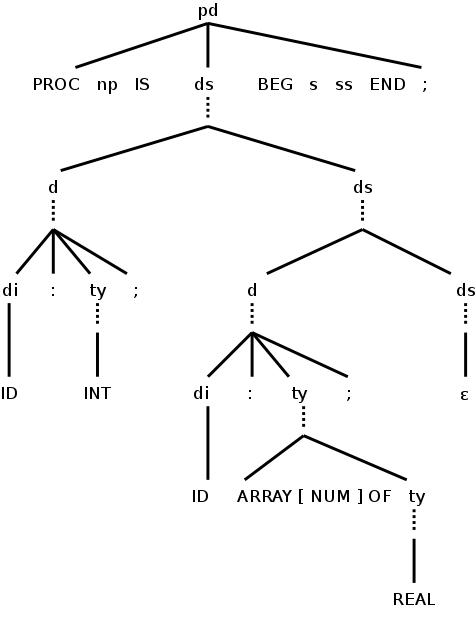
On the right is the parse tree, limited to the declarations.

The dotted lines would be solid for a parse tree and connect to the lines below. They are shown dotted so that the figure can be compared to the annotated parse tree immediately below, in which the attributes and their values have been filled in.

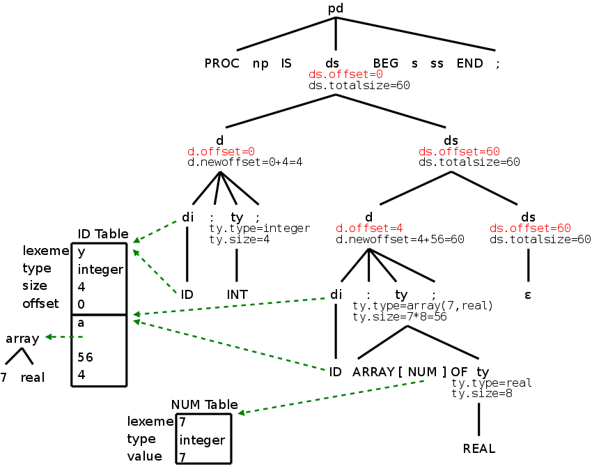
In the annotated tree, the attributes shown in red are inherited. Those in black are synthesized.

To start the annotation process, look at the top production in the parse tree. It has an inherited attributed ds.offset, which is set to zero. Since the attribute is inherited, the entry can be placed immediately into the annotated tree.

We now do the left child and fill in its inherited attribute.

When the Euler tour comes back up the tree, the synthesized attributes are evaluated and recorded.

6.3.6: Fields in Records and Classes

Since records can essentially have a bunch of declarations inside, we only need add

    T → RECORD { D }
  

  T → record {  { Env.push(top);
                  top = new Env();
                  Stack.push(offset);
                  offset = 0; }
  D }           { T.type = record(top);
                  T.width = offset;
                  top = Env.pop();
                  offset = Stack.pop(); }

This does not apply directly to the class grammar, which does not have records.

This same technique would be used for other examples of nested scope, e.g., nested procedures/functions and nested blocks. To have nested procedures/functions, we need other alternatives for declaration: procedure/function definitions. Similarly if we wanted to have nested blocks we would add another alternative to statement.

  s           → ks | ids | block-stmt
  block-stmt  → DECLARE ds BEGIN ss END ;

If we wanted to generate code for nested procedures or nested blocks, we would need to stack the symbol table as done above and in the text.

Homework: 1.

6.4: Translation of Expressions

The goal is to generate 3-address code for scalar expressions, i.e., arrays are not treated in this section (they will be shortly). Specifically, indices is assumed to be ε. We use is to abbreviate indices.

We generate the 3-address code using the natural notation of 6.2. In fact we assume there is a function gen() that, given the pieces needed, does the proper formatting so gen(x = y + z) will output the corresponding 3-address code. gen() is often called with addresses other than lexemes, e.g., temporaries and constants. The constructor Temp() produces a new address in whatever format gen needs. Hopefully this will be clear in the table to the right and the others that follow.

6.4.1: Operations Within Expressions

We will use two attributes code and address (addr). The key objective at each node of the parse tree for an expression is to produce values for the code and addr attributes so that the following crucial invariant is maintained.

If code is executed, then address addr contains the value of the (sub-)expression routed at this node.

Said another way, the attribute addr at a node is the address that holds the value calculated by the code at the node. Recall that unlike real code for a real machine our 3-address code doesn't reuse temporary addresses.

As one would expect for expressions, all the attributes in the table to the right are synthesized. The table is for the expression part of the class grammar. To save space we use ID for IDENTIFIER, e for expression, t for term, and f for factor.

The SDDs for declarations and scalar expressions can be easily combined by essentially concatenating them as shown here.

6.4.3: Addressing Array Elements

The idea is to associate the base address with the array name. That is, the offset stored in the identifier table entry for the array is the address of the first element. When an element is referenced, the indices and the array bounds are used to compute the amount, often called the offset (unfortunately, we have already used that term), by which the address of the referenced element differs from the base address.

To implement this technique, we must first store the base type of each identifier in the identifier table. We use this basetype to determine the size of each element of the array. For example, consider

    arr: array [10] of integer;
    x  : real ;
  

This SDD is combined with the expression SDD here.

One Dimensional Arrays

Calculating the address of an element of a one dimensional array is easy. The address increment is the width of each element times the index (assuming indices start at 0). So the address of A[i] is the base address of A, which is the offset component of A's entry in the identifier table, plus i times the width of each element of A.

The width of each element of an array is the width of what we have called the base type of the array. For a scalar, there is just one element and its width is the width of the type, which is the same as the base type. Hence, for any ID the element width is sizeof(getBaseType(ID.entry)).

For convenience, we define getBaseWidth by the formula

    getBaseWidth(ID.entry) = sizeof(getBaseType(ID.entry)) = sizeof(ID.entry.baseType)
  

Two Dimensional Arrays

Let us assume row major ordering. That is, the first element stored is A[0,0], then A[0,1], ... A[0,k-1], then A[1,0], ... . Modern languages use row major ordering.

With the alternative column major ordering, after A[0,0] comes A[1,0], A[2,0], ... .

For two dimensional arrays the address of A[i,j] is the sum of three terms

1. The base address of A.
2. The distance from A to the start of row i. This is i times the width of a row, which is i times the number of elements in a row times the width of an element. The number of elements in a row is the column array bound.
3. The distance from the start of row i to element A[i,j]. This is j times the width of an element.

Remarks

1. Our grammar really declares one dimensional arrays of one dimensional arrays rather than 2D arrays. I believe this makes it easier.
2. The SDD above when processing the declaration
       A : array [5] of array [9] of real;
   gives A the type array(5,array(9,real)) and thus the type component of the entry for A in the symbol table contains all the values needed to compute the address of any given element of the array.

End of Remarks

Higher Dimensional Arrays

The generalization to higher dimensional arrays is clear.

A Simple Example

Consider the following expression containing a simple array reference, where a and c are integers and b is a real array.

    a = b[3*c]
  

    T1 = 3 * c     // i.e. mult T1,3,c
    T2 = T1 * 8    // each b[i] is size 8
    a  = b[T2]     // Uses the x[i] special form
  

    T1 = 3 * c
    T2 = T1 * 8
    T3 = &b
    T4 = T2 + T3
    a  = *T4
  

6.4.4: Translation of Array References (Within Expressions)

To permit arrays in expressions, we need to specify the semantic actions for the production

    factor → IDENTIFIER indices
  

One-Dimensional Array References

As a warm-up, lets start with references to one-dimensional arrays. That is, instead of the above production, we consider the simpler

    factor → IDENTIFIER index
  

The table on the right does this in two ways, both with and without using the special addressing form x[j]. In the table the nonterminal index is abbreviated i . I included the version without the x[j] special form for two reasons.

1. Since we are restricted to one dimensional arrays, the full code generation for the address of an element is not hard.
2. I thought it would be instructive to see the full address generation without hiding some of it under the covers. It was definitely instructive for me!

Note that by avoiding the special form b=x[j], I ended up using two other special forms.
Is it possible to avoid the special forms?

Our Special Forms for Addressing

We just (optionally) saw an exception to the basic lisp evaluation rule. A similar exception occurs with x[j] in our three-address code. It is a special form in that, unlike the normal rules for three-address code, we don't use the address of j but instead its value. Specifically the value of j is added to the address of x.

The rules for addresses in 3-address code also include

    a = &b
    a = *b
    *a = b
  

Incorporating 1D Arrays in the Expression SDD

Our current SDD includes the production

    f → ID is
  

    f → ID
    f → ID i
  

The semantic rules for each case were given in previous tables. The ensemble to date is given here.

On the board evaluate e.code for the RHS of the simple example above: a=b[3*c].

This is an exciting moment. At long last we really seem to be compiling!

Multidimensional Array References

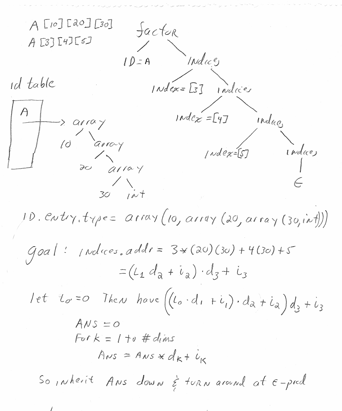
As mentioned above in the general case we must process the production

    f → IDENTIFIER is
  

Following the method used in the 1D case we need to construct is.code. The basic idea is shown here

The Left-Hand Side

Now that we can evaluate expressions (including one-dimensional array reverences) we need to handle the left-hand side of an assignment statement (which also can be an array reference). Specifically we need semantic actions for the following productions from the class grammar.

    id-statement   → ID rest-of-assign
    rest-of-assign → = expression ;
    rest-of-assign → indices = expression
  

Scalars and One Dimensional Arrays on the Left Hand Side

Once again we begin by restricting ourselves to one-dimensional arrays, which corresponds to replacing indices by index in the last production. The SDD for this restricted case is shown on the right.

The first three productions reduce statements (ss) and statement (s) to identifier-statement (ids), which is used for statements such as assignment and procedure invocation, that begin with an identifier. The corresponding semantic rules simply concatenate all the code produced into the top ss.code.

The identifier-statement production captures the ID and sends it down to the appropriate rest-of-assignment (ra) production where the necessary code is generated and passed back up.

The simple ra → := e; production generates ra.code by simply appending to the evaluation of the RHS, the natural assignment with ra as the LHS.

It is instructive to compare ra.code for the ra → i := e production with f.code for the f → ID i production in the expression SDD. Both compute the same offset (index*elementSize) and both use a special form for the address x[j]=y in this section and y=x[j] for expressions.

Incorporating these productions and semantics gives this SDD. Note that we have added a semantic rule to the procedure-def (pd) production. This rule simply concatenates the code in the s and ss symbols appearing between BEG and END

Multi-dimensional Arrays on the Left Hand Side

The idea is the same as when a multidimensional array appears in an expression. Specifically,

1. Traverse the sub-tree routed at the top indices node and compute the total offset from the start of the array.
2. Multiply this offset by the width of each entry.
3. A[product] = RHS

Our Simple Example Revisited

Recall the program we could partially handle.

  procedure P2 is
      y : integer;
      a : array [7] of real;
  begin
      y := 5;      // Statements not yet done
      a[2] := y;   // Type error?
  end;

Now we can do the statements.

Homework: What code is generated for the program written above? Please remind me to go over this homework next class.

What should we do about the possible type error?

1. We could ignore errors.
2. We could assume the intermediate language permits mismatched types. Final code generation would then need to generate conversion code or signal an error.
3. We could change the program to use only one type.
4. We could learn about type checking and conversions.

Let's take the last option.

6.5: Type Checking

Type Checking includes several aspects.

1. The language comes with a type system, i.e., a set of rules saying what types can appear where.
2. The compiler assigns type expressions to parts of the source program.
3. The compiler ensures that the type usage in the program conforms to the type system for the language. This does not mean that the necessary type checks are performed at compile time.

For any language, all type checking could be done at run time, i.e. there would be no compile-time checking. However, that does not mean the compiler is absolved from the type checking. Instead, the compiler generates code to do the checks at run time.

It is normally preferable to perform the checks at compile time, if possible. Some languages have very weak typing; for example, variables can change their type during execution. Often these languages need run-time checks. Examples include lisp, snobol, and apl.

A sound type system guarantees that all checks can be performed prior to execution. This does not mean that a given compiler will make all the necessary checks.

An implementation is strongly typed if compiled programs are guaranteed to run without type errors.

6.5.1: Rules for Type Checking

There are two forms of type checking.

1. We will learn type synthesis where the types of parts are used to infer the type of the whole. For example, integer+real=real.
2. Type inference is very slick. The type of a construct is determined from its usage. This permits languages like ML to check types even though names need not be declared.

We will implement type checking for expressions. Type checking statements is similar. The SDDs below (and for lab 4) contain type checking (and coercions) for assignment statements as well as expressions.

6.5.2: Type Conversions

A very strict type system would do no automatic conversion. Instead it would offer functions for the programmer to explicitly convert between selected types. With such a system, either the program has compatible types or is in error. Such explicit conversions supplied by the programmer are called casts.

We, however, will consider a more liberal approach in which the language permits certain implicit conversions that the compiler is to supply. This is called type coercion.

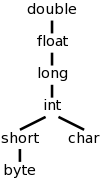
We continue to work primarily with the two basic types integer and real, and postulate a unary function denoted (real) that converts an integer into the real having the same value. Nonetheless, we do consider the more general case where there are multiple types some of which have coercions (often called widenings). For example in C/Java, int can be widened to long, which in turn can be widened to float as shown in the figure to the right.

Mathematically the hierarchy on the right is a partially order set (poset) in which each pair of elements has a least upper bound (LUB). For many binary operators (all the arithmetic ones we are considering, but not exponentiation) the two operands are converted to the LUB. So adding a short to a char, requires both to be converted to an int. Adding a byte to a float, requires the byte to be converted to a float (the float remains a float and is not converted).