Answer: We will need to enforce
declaration before use. So, in expression evaluation, we should check the entry in the identifier table to be sure that the type has already been set.
Start Lecture #9
A good summary of the available techniques.
preorderis relevant).
Recall that in fully-general, recursive-descent parsing one normally writes one procedure for each nonterminal.
Assume the SDD is L-attributed.
We are interested in using predictive parsing for LL(1) grammars In this case we have a procedure P for each production, which is implemented as follows.
Assume we have the parse tree on the right as produced, for example, by your lab3. (The numbers should really be a token, e.g. NUM, not the lexemes shown.) You now want to write the semantics analyzer, or intermediate code generator, or lab 4. In any of these cases you have semantic rules or actions (for lab4 it will be semantic rules) that need to be performed. Assume the SDD or SDT is L-attributed (that is my job for lab4), so we don't have to worry about dependence loops.
You start to write
analyze-i.e.-traverse (tree-node)
which will be initially called with tree-node=the-root.
The procedure will perform an Euler-tour traversal of the parse tree
and during its visits of the nodes, it will evaluate the relevant
semantic rules.
The visit() procedure is basically a big switch statement where the cases correspond to evaluating the semantic rules for the different productions in the grammar. The tree-node is the LHS of the production and the children are the RHS.
By first switching on the tree-node and then inspecting enough of the children, visit() can tell which production the tree-node corresponds to and which semantic rules to apply.
As described in 5.5.1 above, visit() has received as parameters (in addition to tree-node), the inherited attributes of the node. The traversal calls itself recursively, with the tree-node argument set to the leftmost child, then calls again using the next child, etc. Each time, the child is passed the inherited attributes.
When each child returns, it passes back its synthesized attributes.
After the last child returns, the parent returns, passing back the synthesized attributes that were calculated.
A programming point is that, since tree-node can be any node, traverse() and visit() must each be prepared to accept as parameters any inherited attribute that any nonterminal can have.
Instead of a giant switch, you could have separate routines for each nonterminal and just switch on the productions having this nonterminal as LHS.
In this case each routine need be prepared to accept as parameters only all the inherited attributes that its nonterminal can have.
You could have separate routines for each production and thus each routine has as parameters exactly the inherited attributes that this production receives.
To do this requires knowing which visit() procedure to call for
each nonterminal (child node of the tree).
For example, assume you are processing the production
B → C D
You need to know which production to call for C
(remember that C can be the LHS of many different productions).
Homework: Read Chapter 6.
The difference between a syntax DAG and a syntax tree is that the
former can have undirected cycles.
DAGs are useful where there are multiple, identical portions in a
given input.
The common case of this is for expressions where there often are
common subexpressions.
For example in the expression
X + a + b + c - X + ( a + b + c )
each individual variable is a common subexpression.
But a+b+c is not since the first occurrence has the X already
added.
This is a real difference when one considers the possibility of
overflow or of loss of precision.
The easy case is
x + y * z * w - ( q + y * z * w )
where y*z*w is a common subexpression.
It is easy to find such common subexpressions. The constructor Node() above checks if an identical node exists before creating a new one. So Node ('/',left,right) first checks if there is a node with op='/' and children left and right. If so, a reference to that node is returned; if not, a new node is created as before.
Homework: 1.
Often one stores the tree or DAG in an array, one entry per node.
Then the array index, rather than a pointer, is used to reference a
node.
This index is called the node's value-number and the triple
<op, value-number of left, value-number of right>
is called the signature of the node.
When Node(op,left,right) needs to determine if an identical node
exists, it simply searches the table for an entry with the required
signature.
Searching an unordered array is slow; there are many better data structures to use. Hash tables are a good choice.
Homework: 2.
We will use three-address code, i.e., instructions of the
form op a,b,c, where op is a primitive
operator.
For example
    lshift a,b,4   // left shift b by 4 and place result in a
    add    a,b,c   // a = b + c
    a = b + c      // alternate (more natural) representation of above
If we are starting with an expression DAG (or syntax tree if less aggressive), then transforming into 3-address code is just a topological sort and an assignment of a 3-address operation with a new name for the result to each interior node (the leaves already have names and values).
A key point is that nodes in an expression dag (or tree) have at most 2 children so three-address code is easy. As we produce three-address code for various constructs, we may have to generate several instructions to translate one construct.
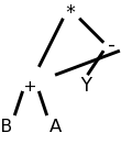
For example, (B+A)*(Y-(B+A)) produces the DAG on the right, which yields the following 3-address code.
    t1 = B + A
    t2 = Y - t1
    t3 = t1 * t2
Notes
We use the terminology 3-address code since instructions in our
intermediate-language consist of one elementary
operation
with three operands, each of which is often an address.
Typically two of the addresses represent source operands or
arguments of the operation and the third represents the result.
Some of the 3-address operations have fewer than three addresses; we
simply think of the missing addresses as unused (or ignored) fields
in the instruction.
Consider
Q := Z; or
A[f(x)+B*D] := g(B+C*h(x,y));.
Where [] indicates array reference and () indicates a function call.
From a macroscopic view, performing each assignment involves three tasks.
Note the differences between L-values, quantities that can appear on the LHS of an assignment, and and R-values, quantities that can appear only on the RHS.
There is no universally agreed to set of three-address instructions, or even whether 3-address code should be the intermediate code for the compiler. Some prefer a set close to a machine architecture. Others prefer a higher-level set closer to the source, for example, subsets of C have been used. Others prefer to have multiple levels of intermediate code in the compiler and define a compilation phase that converts the high-level intermediate code into the low-level intermediate code. What follows is the set proposed in the book.
In the list below, x, y, and z are addresses; i is an integer,
not an address); and L is a symbolic label.
The instructions can be thought of as numbered and the labels can be
converted to the numbers with another pass over the output or
via backpatching
, which is discussed below.
	param S
	param U
	param V
	t = call G,2
	param t
	param W
	A = call F,3
Indexed Copy ops. x = y[i] x[i] =
y.
In the second example, x[i] is the address that is
the-value-of-i locations after the address x; in particular
x[0] is the same address as x.
Similarly for y[i] in the first example.
But a crucial difference is that, since y[i] is on the RHS,
the address is dereferenced and the value in the
address is what is used.
Note that x[i] = y[j] is not permitted as that requires 4 addresses. x[i] = y[i] could be permitted, but is not.
Quads are an easy, almost obvious, way to represent the three address instructions: put the op into the first of four fields and the three addresses into the remaining three fields. Some instructions do not use all the fields. Many operands will be references to entries in tables (e.g., the identifier table).
A triple optimizes
a quad by eliminating the result field of
a quad since the result is often a temporary.
When this result occurs as a source operand of a subsequent instruction, the source operand is written as the value-number of the instruction yielding this result (distinguished some way, say with parens).
If the result field of a quad is a program name and not a temporary then two triples may be needed:
When an optimizing compiler reorders instructions for increased performance, extra work is needed with triples since the instruction numbers, which have changed, are used implicitly. Hence the triples must be regenerated with correct numbers as operands.
With Indirect triples we maintain an array of pointers to triples and, if it is necessary to reorder instructions, just reorder these pointers. This has two advantages.
Homework: 1, 2 (you may use the parse tree instead of the syntax tree if you prefer).
This has become a big deal in modern optimizers, but we will
largely ignore it.
The idea is that you have all assignments go to unique (temporary)
variables.
So if the code is
if x then y=4 else y=5
it is treated as though it was
if x then y1=4 else y2=5
The interesting part comes when y is used later in the program and
the compiler must choose between y1 and y2.
Much of the early part of this section is really about programming languages more than about compilers.
A type expression is either a basic type or the result of applying a type constructor.
There are two camps, name equivalence and structural equivalence.
Consider the following example.
    declare
       type MyInteger is new Integer;
       MyX : MyInteger;
       x   : Integer := 0;
    begin
       MyX := x;
    end
This generates a type error in Ada, which has name equivalence since
the types of x and MyX do not have the same name, although they have
the same structure.
As another example, consider an object of an anonymous
type
as in
X : array [5] of integer;
X does not have the same type as any other object not even Y
declared as
y : array [5] of integer;
However, x[2] has the same type as y[3]; both are integers.
The following example from the 2e uses an usual C/Java-like array notation. (The 1e had pascal-like notation.) Although I prefer Ada-like constructs as in lab 3, I realize that the class knows C/Java best so like the authors I will sometimes follow the 2e as well as presenting lab3-like grammars. I will often refer to lab3-like grammars as the class grammar.
The grammar below gives C/Java-like records/structs/methodless-classes as well as multidimensional arrays (really singly dimensioned arrays of singly dimensioned arrays).
    D → T id ; D | ε
    T → B C | RECORD { D }
    B → INT | FLOAT
    C → [ NUM ] C | ε
Note that an example sentence derived from D is
int [5] x ;
which is not legal C, but does have the virtuethat the type is separate from identifier being declared.
The class grammar doesn't support records. This part of the class grammar declares ints, reals, arrays, and user-defined types.
    declarations         → declaration declarations | ε
    declaration          → defining-identifier : type ; |
                           TYPE defining-identifier IS type ;
    defining-identifier  → IDENTIFIER
    type                 → INT | REAL | ARRAY [ NUMBER ] OF type | IDENTIFIER
So that the tables below are not too wide, let's use shorter names
for the nonterminals.
Specifically, we abbreviate declaration as d, declarations as ds,
defining-identifier, as di, and type as ty (unfortunately, we have
already used t to abbreviate term).
For now we ignore the second possibility for a declaration (declaring a type itself).
ds → d ds | ε
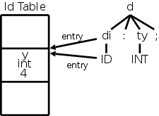
d → di : ty ;
di → ID
ty → INT | REAL | ARRAY [ NUMBER ] OF ty
It is useful to support user-declared types. For example
      type vector5 is array [5] of real;
      v5 : vector5;
The full class grammar does support this.
      ds   → d ds | ε
      d    → di : ty ; | TYPE di IS ty ;
      di   → ID
      ty   → INT | REAL | ARRAY [ NUMBER ] OF ty | ID
Ada supports both constrained array types such as
type t1 is array [5] of integer;
and unconstrained array types such as
type t2 is array of integer;
With the latter, the constraint is specified when the array (object)
itself is declared.
      x1 : t1
      x2 : t2[5]
You might wonder why we want the unconstrained type. These types permit a procedure to have a parameter that is an array of integers of unspecified size. Remember that the declaration of a procedure specifies only the type of the parameter; the object is determined at the time of the procedure call.
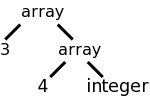
Previously we considered an SDD for
arrays that was able to compute the type.
The key point was that it called the function array(size,type) so as
to produce a tree structure exhibiting the dimensionality of the
array.
For example the tree on the right would be produced for
int[3][4]
or array [3] of array [4] of int.
Now we will extend the SDD to calculate the size of the array as well. For example, the array pictured has size 48, assuming that each int has size 4. When we declare many objects, we need to know the size of each one in order to determine the offsets of the objects from the start of the storage area.
We are considering here only those types for which the storage requirements can be computed at compile time. For others, e.g., string variables, dynamic arrays, etc, we would only be reserving space for a pointer to the structure; the structure itself would be created at run time. Such structures are discussed in the next chapter.
| Production | Actions | Semantic Rules |
|---|---|---|
| T → B | { t = B.type } | C.bt = B.bt |
| { w = B.width } | C.bw = B.bw | |
| C | { T.type = C.type } | T.type = C.type |
| { T.width = B.width; } | T.width = C.width | |
| B → INT | { B.type = integer; B.width = 4; } | B.bt = integer B.bw = 4 |
| B → FLOAT | { B.type = float; B.width = 8; } | B.bt = float B.bw = 8 |
| C → [ NUM ] C1 | C.type = array(NUM.value, C1.type) | |
| C.width = NUM.value * C1.width; | ||
| { C.type = array(NUM.value, C1.type); | C1.bt = C.bt | |
| C.width = NUM.value * C1.width; } | C1.bw = C.bw | |
| C → ε | { C.type = t; C.width=w } | C.type = C.bt C.width = C.bw |
The idea (for arrays whose size can be determined at compile time)
is that the basic type determines the width of the object, and the
number of elements in the array determines the height
.
These are then multiplied to get the size (area) of the object.
The terminology actually used is that the basetype determines the
basewidth, which when multiplied by the number of elements gives the
width.
The book uses semantic actions, i.e., a syntax directed translation or SDT. I added the corresponding semantic rules so that the table to the right is an SDD as well. In both cases we follow the book and show a single type specification T rather than a list of object declarations D. The omitted productions are
D → T ID ; D | ε
The goal of the SDD is to calculate two attributes of the start symbol T, namely T.type and T.width, the rules can be viewed as the implementation.
The basetype and hence the basewidth are determined by B, which is INT or FLOAT. The values are set by the lexer (as attributes of FLOAT and INT) or, as shown in the table, are constants in the parser. NUM.value is set by the lexer.
These attributes of B pushed down the tree via the inherited
attributes C.bw and C.bw until all the array dimensions have been
passed over and the ε-production is reached.
There they are turned around
as usual and sent back up,
during which the dimensions are processed and the final type and
width are calculated.
An alternative implementation, using global variables, is described in the grayed out description of the semantic actions This is similar to the comment above that instead of having the identifier table passed up and down via attributes, the bullet can be bitten and a globally visible table used instead.
Remember that for an SDT, the placement of the actions within the production is important. Since it aids reading to have the actions lined up in a column, we sometimes write the production itself on multiple lines. For example the production T→BC in the table below has the B and C on separate lines so that (the first two) actions can be in between even though they are written to the right. These two actions are performed after the B child has been traversed, but before the C child has been traversed. The final two actions are at the very end so are done after both children have been traversed.
The actions use global variables t and w to carry the base type (INT or FLOAT) and width down to the ε-production, where they are then sent on their way up and become multiplied by the various dimensions.
| Production | Semantic Rules (All Attributes Synthesized) |
|---|---|
| d → di : ty ; | addType(di.entry, ty.type); addSize(di.entry, ty.size) |
| di → ID | di.entry = ID.entry |
| ty → ARRAY [ NUM ] OF ty1 ; | ty.type = array(NUM.value, ty1.type) ty.size = NUM.value * ty1.size |
| ty → INT | ty.type = integer ty.size = 4 |
| ty → REAL | ty.type = real ty.size = 8 |
This exercise is easier with the class grammar since there are no inherited attributes. We again assume that the lexer has defined NUM.value (it is likely a field in the numbers table entry for the token NUM). The goal is to augment the identifier table entry for ID to include the type and size information found in the declaration. This can be written two ways.
Recall that addType is viewed as synthesized since its parameters come from the RHS, i.e., from children of this node.
addType has a side effect (it modifies the identifier table) so we must ensure that we do not use this table value before it is calculated.
When do we use this value?
Answer: When we evaluate expressions, we will need to look up the
types of objects.
How can we ensure that the type has already been determined and
saved?
Answer: We will need to enforce declaration before use
.
So, in expression evaluation, we should check the entry in the
identifier table to be sure that the type has already been set.
Example 1:
As a simple example, let us construct,
on the board, the parse tree for the scalar declaration
y : int ;
We get the diagram at the right, in which I have also shown the
effects of the semantic rules.
Note specifically the effect of the addType and addSize functions on the identifier table.
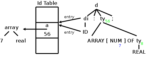
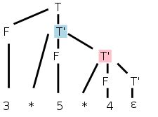
Example 2:
For our next example we choose the array declaration
a : array [7] of int ;
The result is again shown on the right.
The green numbers show the value of t.size and the blue number shows
the value of NUM.value.
Example 3:
For our final example in this section we combine the two previous
declarations into the following simple complete program.
In this example we show only the parse tree.
In the next section we consider the semantic actions as well.
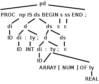
    Procedure P1 is
      y : int;
      a : array [7] of real;
    begin
    end;
Procedure P1 is in fact illegal since the lab3 grammar requires a
statement between begin and end, but let's pretend that we have the
additional productionWe observe several points about this example.
Remark: Be careful to distinguish between three methods used to store and pass information.
To summarize, the identifier table (and other tables we have used) are not present when the program is run. But there must be run time storage for objects. In addition to allocating the storage (a subject discussed next chapter), we need to determine the address each object will have during execution. Specifically, we need to know its offset from the start of the area used for object storage.
For just one object, it is trivial: the offset is zero. When there are multiple objects, we need to keep a running sum of the sizes of the preceding objects, which is our next objective.
The goal is to permit multiple declarations in the same procedure (or program or function). For C/java like languages this can occur in two ways.
In either case we need to associate with each object being declared the location in which it will be stored at run time. Specifically we include in the table entry for the object, its offset from the beginning of the current procedure. We initialize this offset at the beginning of the procedure and increment it after each object declaration.
The lab3 grammar does not support multiple objects in a single declaration.
C/Java does permit multiple objects in a single declaration, but surprisingly the 2e grammar does not.
Naturally, the way to permit multiple declarations is to have a
list of declarations in the natural right-recursive way.
The 2e C/Java grammar has D which is a list of semicolon-separated
T ID's
D → T ID ; D | ε
The lab 3 grammar has a list of declarations
(each of which ends in a semicolon).
Shortening declarations to ds we have
ds → d ds | ε
| Production | Semantic Action |
|---|---|
| P → | { offset = 0; } |
| D | |
| D → T ID ; | { top.put(id.lexeme, T.type, offset); |
| offset = offset + T. width; } | |
| D1 | |
| D → ε |
As mentioned, we need to maintain an offset, the next storage location to be used by an object declaration. The 2e snippet on the right introduces a nonterminal P for program that gives a convenient place to initialize offset.
The name top is used to signify that we work with the top symbol table (when we have nested scopes for record definitions, nested procedures, or nested blocks we need a stack of symbol tables). Top.put places the identifier into this table with its type and storage location and then bumps offset for the next variable or next declaration.
Rather than figure out how to put this snippet together with the previous 2e code that handled arrays, we will just present the snippets and put everything together on the lab 3 grammar.