Compilers
Start Lecture #14
8.1.4: Register Allocation
Since registers are the fastest memory in the computer, the ideal
solution is to store all values in registers.
However, there are normally not nearly enough registers for this to
be possible.
So we must choose which values are in the registers at any given time.
Actually this problem has two parts.
- Which values should be stored in registers?
- Which register should each selected value be stored in
The reason for the second problem is that often there are register
requirements, e.g., floating-point values in floating-point
registers and certain requirements for even-odd register pairs
(e.g., 0&1 but not 1&2) for multiplication/division.
8.1.5: Evaluation Order
Sometimes better code results if the quads are reordered.
One example occurs with modern processors that can execute multiple
instructions concurrently, providing certain restrictions are met
(the obvious one is that the input operands must already be
evaluated).
8.2: The Target Language
This is a delicate compromise between RISC and CISC.
The goal is to be simple but to permit the study of nontrivial
addressing modes and the corresponding optimizations.
A charging
scheme is instituted to reflect that complex addressing
modes are not free.
8.2.1: A Simple Target Machine Model
We postulate the following (RISC-like) instruction set
-
Load. LD dest, addr
loads the destination dest with the contents of the
address addr.
LD reg1, reg2 is a register copy.
A question is whether dest can be a memory location or whether
it must be a register.
This is part of the RISC/CISC debate.
In CISC parlance, no distinction is made between load and
store, both are examples of the general move instruction that
can have an arbitrary source and an arbitrary destination.
We will normally not use a memory location for the
destination of a load (or the source of a store).
This implies that we are not able to perform a memory to memory
copy in one instruction.
As will be seen below we charge more for accessing memory
location than for a register.
-
Store. ST addr, src
stores the value of the source src (register) into
the address addr.
-
Computation. OP dest, src1, src2
or dest = src1 OP src2
performs the operation OP on the two source operands src1 and
src2.
For a RISC architecture the three operands must be registers.
If the destination is one of the sources, the source is read
first and then overwritten (in one cycle by utilizing a
master-slave flip-flop, when both are registers).
-
Unconditional branch. BR L
transfers control to the (instruction with) label L.
When used with an address rather than a label it means to
goto that address.
Note that we are using the l-value of the address.
This is unlike the situation with a load instruction in which
case the r-value i.e., the contents of the
address, is loaded into the register.
-
Conditional Branch. Bcond r, L
transfers to the label L if register r satisfies the
condition cond.
For example,
BNEG R0, joe
branches to joe if R0 is negative.
Addressing modes
The addressing modes are not simply RISC-like, as they permit
indirection through memory locations.
Again, note that we shall charge extra for some such operands.
Recall the difference between an l-value and an r-value, e.g. the
difference between the uses of x in
x = y + 3
and
z = x + 12x
The first refer to an address, the second to a value
(stored in that address).
We assume the machine supports the following addressing modes.
-
Variable name.
This is shorthand (or assembler-speak) for the memory location
containing x, i.e., we use the l-value of the variable name.
So
LD R1, a
sets the contents of R1 equal to the contents of a, i.e.,
contents(R1) := contents(a)
Do not get confused here.
The l-value of a is used as the address (that is what the
addressing mode tells us).
But the load instruction itself loads the first operand with
the contents of the second.
That is why it is the r-value of the second operand that is
placed into the first operand.
-
Indexed address.
The address a(reg), where a is a variable name and reg is a
register (i.e., a register number), specifies the address that
is the r-value-of-reg bytes past the address specified by a.
That is, the address is computed as the l-value of a plus the
r-value of reg.
So
LD r1, a(r2)
sets
contents(r1) := contents(a+contents(r2))
NOT
contents(r1) := contents(contents(a)+contents(r2))
Permitting this addressing mode outside a load or store
instruction would strongly suggest a CISC architecture.
-
Indexed constant.
An integer constant can be indexed by a register.
So
LD r1, 8(r4)
sets
contents(r1) := contents(8+contents(r4)).
-
Indirect addressing.
If I is an integer constant and r is a register
(number), the previous addressing mode tells us that I(r)
refers to the address I+contents(r).
The new addressing mode *I(r) refers to the address
contents(I+contents(r)).
The address *r is shorthand for *0(r).
The address *10 is shorthand for
*10(fakeRegisterContainingZero).
So
LD r1, *r2
sets (get ready)
contents(r1) := contents(contents(contents(r2)))
and
LD r1, *50(r2)
sets
contents(r1) := contents(contents(50+contents(r2))).
and
LD r1, *10
sets
contents(r1) := contents(contents(10))
-
Immediate constant.
If a constant is preceded by a # it is treated as an r-value
instead of as a register number.
So
ADD r2, r2, #1
is an increment instruction.
Indeed
ADD 2, 2, #1
does the same thing, but we probably won't write that; for
clarity we will normally write registers beginning with an
r

Addressing Mode Usage
Remember that in 3-address instructions, the variables written are
addresses, i.e., they represent l-values.
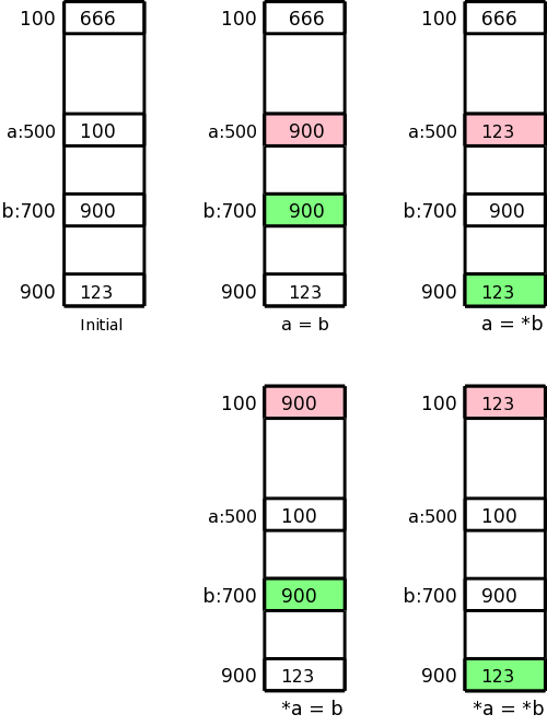
Let us assume the l-value of a is 500 and the l-value b is 700,
i.e., a and b refer to locations 500 and 700 respectively.
Assume further that location 100 contains 666, location 500 contains
100, location 700 contains 900, and location 900 contains 123.
This initial state is shown in the upper left picture.
In the four other pictures the contents of the pink location has
been changed to the contents of the light green location.
These correspond to the three-address assignment statements shown
below each picture.
The machine instructions indicated below implement each of these
assignment statements.
  a = b
      LD  R1, b
      ST  a, R1

  a = *b
      LD  R1, b
      LD  R1, 0(R1)
      ST  a, R1

  *a = b
      LD  R1, b
      LD  R2, a
      ST  0(R2), R1

  *a = *b
      LD  R1, b
      LD  R1, 0(R1)
      LD  R2, a
      ST  0(R2), R1
Naive Translation of Quads to Instructions
For many quads the naive (RISC-like) translation is 4 instructions.
- Load the first source into a register.
- Load the second source into another register.
- Do the operation.
- Store the result.
Array assignment statements are also four instructions.
We can't have a quad A[i]=B[j] because that needs four addresses and
quads have only three.
Similarly, we can't use an array in a computation statement like
a[i]=x+y because it again would need four addresses.
The instruction x=A[i] becomes (assuming each element of A is 4
bytes; our intermediate code generator already does the
multiplication so we would not generate a multiply here).
    LD  R0, i
    MUL R0, R0, #4
    LD  R0, A(R0)
    ST  x, R0
Similarly A[i]=x becomes (again our intermediate code generator
already does the multiplication).
    LD  R0, x
    LD  R1, i
    MUL R1, R1, #4
    ST  A(R1), R0
The (C-like) pointer reference x = *p becomes
    LD  R0, p
    LD  R0, 0(R0)
    ST  x, R0
The assignment through a pointer *p = x becomes
    LD  R0, x
    LD  R1, p
    ST  0(R1), R0
Finally, if x < y goto L becomes
    LD   R0, x
    LD   R1, y
    SUB  R0, R0, R1
    BNEG R0, L
Conclusion
With not much additional effort much of the output of lab 4 could
be turned into naive assembly language.
We will not do this.
Instead, we will spend the little time remaining learning how to
generate less-naive assembly language.
8.2.2: Program and Instruction Costs
Generating good code requires that we have a metric, i.e., a way of
quantifying the cost of executing the code.
The run-time cost of a program depends on (among other factors)
- The cost of the generated instructions.
- The number of times the instructions are executed.
Here we just determine the first cost, and use quite a simple metric.
We charge for each instruction one plus the cost of each addressing
mode used.
Addressing modes using just registers have zero cost, while those
involving memory addresses or constants are charged one.
This corresponds to the size of the instruction since a memory
address or a constant is assumed to be stored in a word right after
the instruction word itself.
You might think that we are measuring the memory (or space) cost of
the program not the time cost, but this is mistaken:
The primary space cost is the size of the data, not the size of the
instructions.
One might say we are charging for the pressure on the I-cache.
For example, LD R0, *50(R2) costs 2, the additional cost is for the
constant 50.
I believe that the book special cases the addresses 0(reg) and
*0(reg) so that the 0 is not explicitly stored and not charged for.
The significance for us is calculating the length an instruction such
as
LD R1, 0(R2)
We care about the length of an instruction when we need to generate
a branch that skips over it.
Homework: 1, 2c, 3, 4.
Calculate the cost for 2c.
8.3: Address in the Target Code
There are 4 possibilities for addresses that must be generated
depending on which of the following areas the address refers to.
- The text or code area.
The location of items in this area is statically determined,
i.e., is known at compile time.
- The static area holding global constants.
The location of items in this area is statically determined.
-
The stack holding activation records.
The location of items in this area is not known at compile time.
-
The heap.
The location of items in this area is not known at compile time.
8.3.1: Static Allocation
Returning to the glory days of Fortran, we first consider a system
with only static allocation.
Remember, that with static allocation we know before execution where
all the data will be stored.
There are no recursive procedures; indeed, there is no run-time
stack of activation records.
Instead the ARs (one per procedure) are statically
allocated by the compiler.
Caller Calling Callee
In this simplified situation, calling a parameterless procedure just
uses static addresses and can be implemented by two instructions.
Specifically,
call procA
can be implemented by
    ST  callee.staticArea, #here+20
    BR  callee.codeArea
Assume, for convenience, that the return address is the
first location in the activation record (in general, for a
parameterless procedure, the return address would be a
fixed offset from the beginning of the AR).
We use the attribute staticArea for the address of the AR for the
given procedure (remember again that there is no stack and no heap).
What is the mysterious #here+20?
The # we know signifies an immediate constant.
We use here to represent the address of the current
instruction (the compiler knows this value since we are assuming
that the entire program, i.e., all procedures, are compiled at
once).
The two instructions listed contain 3 constants, which means that
the entire sequence takes 5 words or 20 bytes.
Thus here+20 is the address of the instruction after the BR, which
is indeed the return address.
Callee Returning
With static allocation, the compiler knows the address of the
the AR for the callee and we are assuming that the return address is
the first entry.
Then a procedure return is simply
BR *callee.staticArea
Let's make sure we understand the indirect addressing here.
The value callee.staticArea is the address of a memory location
into which the caller placed the return address.
So the branch is not to callee.staticArea, but instead to the
return address, which is the value contained in
callee.staticArea.
Example
We consider a main program calling a procedure P and then
halting.
Other actions by Main and P are indicated by subscripted uses
of other
.
  // Quadruples of Main
  other1
  call P
  other2
  halt
  // Quadruples of P
  other3
  return
Let us arbitrarily assume that the code for Main starts in location
1000 and the code for P starts in location 2000 (there might be
other procedures in between).
Also assume that each otheri requires 100 bytes (all
addresses are in bytes).
Finally, we assume that the ARs for Main and P begin at 3000 and
4000 respectively.
Then the following machine code results.
// Code for Main
1000: Other1
1100: ST 4000, #1120 // P.staticArea, #here+20
1112: BR 2000 // Two constants in previous instruction take 8 bytes
1120: other2
1220: HALT
...
// Code for P
2000: other3
2100: BR *4000
...
// AR for Main
3000: // Return address stored here (not used
)
3004: // Local data for Main starts here
...
// AR for P
4000: // Return address stored here
4004: // Local data for P starts here
8.3.2: Stack Allocation
We now need to access the ARs from the stack.
The key distinction is that the location of the current AR
is not known at compile time.
Instead a pointer to the stack must be maintained dynamically.
We dedicate a register, call it SP, for this purpose.
In this chapter we let SP point to the bottom of the current AR,
that is the entire AR is above the SP.
Since we are not supporting varargs, there is no advantage to having
SP point to the middle
of the AR as in the previous chapter.
The main procedure (or the run-time library code called before
any user-written procedure) must initialize SP with
LD SP, #stackStart
where stackStart is a known-at-compile-time constant.
The caller increments SP (which now points to the beginning of its
AR) to point to the beginning of the callee's AR.
This requires an increment by the size of
the caller's AR, which of course the caller knows.
Is this size a compile-time constant?
The book treats it as a constant.
The only part that is not known at compile time is the size of the
dynamic arrays.
Strictly speaking this is not part of the AR, but it must be skipped
over since the callee's AR starts after the caller's dynamic arrays.
Perhaps for simplicity we are assuming that there are no dynamic
arrays being stored on the stack.
If there are arrays, their size must be included in some way.
Caller Calling Callee
The code generated for a parameterless call is
  ADD SP, SP, #caller.ARSize
  ST  0(SP), #here+16        // save return address (book wrong)
  BR  callee.codeArea
Callee Returning
The return requires code from both the Caller and Callee.
The callee transfers control back to the caller with
BR *0(SP)
Upon return the caller restore the stack pointer with
SUB SP, SP, caller.ARSize
Example
We again consider a main program calling a procedure P and then
halting.
Other actions by Main and P are indicated by subscripted uses of
`other'.
  // Quadruples of Main
  other1
  call P
  other2
  halt
  // Quadruples of P
  other3
  return
Recall our assumptions that the code for Main starts in location
1000, the code for P starts in location 2000, and each
otheri requires 100 bytes.
Let us assume the stack begins at 9000 (and grows to larger
addresses) and that the AR for Main is of size 400 (we don't need
P.ARSize since P doesn't call any procedures).
Then the following machine code results.
  // Code for Main
  1000; LD  SP, 9000        // Probably done prior to Main
  1008: Other1
  1108: ADD SP, SP, #400
  1116: ST  0(SP), #1132    // Understand the address
  1124: BR, 2000
  1132: SUB SP, SP, #400
  1140: other2
  1240: HALT
        ...
  // Code for P
  2000: other3
  2100: BR *0(SP)           // Understand the *
        ...
  // AR for Main
  9000:                     // Return address stored here (not used)
  9004:                     // Local data for Main starts here
  9396:                     // Last word of the AR is bytes 9396-9399
        ...
  // AR for P
  9400:                     // Return address stored here
  9404:                     // Local data for P starts here
Homework: 1, 2d, 3c.
8.3.3: Run-Time Addresses for Names
Basically skipped.
A technical fine point about static allocation and a
corresponding point about the display.
8.4: Basic Blocks and Flow Graphs
As we have seen, for many quads it is quite easy to generate a
series of machine instructions to achieve the same effect.
As we have also seen, the resulting code can be quite inefficient.
For one thing the last instruction generated for a quad is often a
store of a value that is then loaded right back in the next quad (or
one or two quads later).
Another problem is that we don't make much use of the registers.
That is, translating a single quad needs just one or two registers so
we might as well throw out all the other registers on the machine.
Both of the problems are due to the same cause:
Our horizon is too limited.
We must consider more than one quad at a time.
But wild flow of control can make it unclear which quads
are dynamically
near each other.
So we want to consider, at one time, a group of quads for which
the dynamic order of execution is tightly controlled.
We then also need to understand how execution proceeds from one
group to another.
Specifically the groups are called basic blocks and the
execution order among them is captured by the flow graph.
Definition:
A basic block is a maximal collection of consecutive quads
such that
- Control enters the block only at the first instruction.
- Branches (or halts) occur only at the last instruction.
Definition:
A flow graph has the basic blocks as vertices and has edges
from one block to each possible dynamic successor.
We process all the quads in a basic block together
making
use of the fact that the block is not entered or left in
the middle
.
8.4.1: Basic Blocks
Constructing the basic blocks is easy.
Once you find the start of a block, you keep going until you hit a
label or jump.
But, as usual, to say it correctly takes more words.
Definition:
A basic block leader (i.e., first instruction) is any of the
following (except for the instruction just past the entire program).
- The first instruction of the program.
- A target of a (conditional or unconditional) jump.
- The instruction immediately following a jump.
Given the leaders, a basic block starts with a leader and proceeds
up to but not including the next leader.
Example
The following code produces a 10x10 real identity matrix
    for i from 1 to 10 do
      for j from 1 to 10 do
        a[i,j] = 0
      end
    end
    for i from 1 to 10 do
      a[i,i] = 1.0
    end
The following quads do the same thing.
Don't worry too much about how the quads were generated.
     1)  i = 1
     2)  j = 1
     3)  t1 = 10 * i
     4)  t2 = t1 + j        // element [i,j]
     5)  t3 = 8 * t2        // offset for a[i,j] (8 byte reals)
     6)  t4 = t3 - 88       // program array starts at [1,1] assembler at [0,0]
     7)  a[t4] = 0.0
     8)  j = j + 1
     9)  if j <= 10 goto (3)
    10)  i = i + 1
    11)  if i <= 10 goto (2)
    12)  i = 1
    13)  t5 = i - 1
    14)  t6 = 88 * t5
    15)  a[t6] = 1.0
    16)  i = i + 1
    17)  if i <= 10 goto (13)
Which quads are leaders?
1 is a leader by definition.
The jumps are 9, 11, and 17.
So 10 and 12 are leaders as are the targets 3, 2, and 13.
The leaders are then 1, 2, 3, 10, 12, and 13.
The basic blocks are therefore {1}, {2}, {3,4,5,6,7,8,9}, {10,11},
{12}, and {13,14,15,16,17}.
Here is the code written again with the basic blocks indicated.
     1)  i = 1

     2)  j = 1

     3)  t1 = 10 * i
     4)  t2 = t1 + j            // element [i,j]
     5)  t3 = 8 * t2            // offset for a[i,j] (8 byte numbers)
     6)  t4 = t3 - 88           // we start at [1,1] not [0,0]
     7)  a[t4] = 0.0
     8)  j = j + 1
     9)  if J <= 10 goto (3)

    10)  i = i + 1
    11)  if i <= 10 goto (2)

    12)  i = 1

    13)  t5 = i - 1
    14)  t6 = 88 * t5
    15)  a[t6] = 1.0
    16)  i = i + 1
    17)  if i <= 10 goto (13)
We can see that once you execute the leader you are assured of
executing the rest of the block in order.
8.4.2: Next Use Information
We want to record the flow of information from instructions that
compute a value to those that use the value.
One advantage we will achieve is that if we find a value has no
subsequent uses, then it is dead and the register holding that value
can be used for another value.
Assume that a quad p assigns a value to x (some would call this
a def of x).
Definition:
A quad q uses the value computed at p (uses
the def) and x is live at q
if q has x as an operand and there is a possible execution path from
p to q that does not pass any other def of x.
Since the flow of control is trivial inside a basic block, we are
able to compute the live/dead status and next use information at the
block leader by a simple backwards scan of the quads (algorithm
below).
Note that if x is dead (i.e., defined before used) on entrance to B
the register containing x can be reused in B.
Computing Live/Dead and Next Use Information
Our goal is to determine whether a block uses a value and if so in
which statement.
The following algorithm for computing uses is quite simple.
    Initialize all variables in B as being live
    Examine the quads of the block in reverse order.
        Assume the quad q computes x and reads y and z
        Mark x as dead; mark y and z as live and used at q
When the loop finishes those values that are read before being
written are marked as live and their first use is noted.
The locations x that are written before being read are marked dead
meaning that the value of x on entrance is not used.

8.4.3: Flow Graphs
The nodes of the flow graph are the basic blocks and there is an
edge from P (predecessor) to S (successor) if S might follow P
More formally, such an edge is added if the last statement of P
- is a jump to S (it must be to the leader of S) or
- is not an unconditional jump and S immediately follows P.
Two nodes are added: entry
and exit
.
An edge is added from entry to the first basic block, i.e. the block
that has the first statement of the program as leader.
Edges to the exit are added from any block that could be the last
block executed.
Specifically, edges are added to exit from
- the last block if it doesn't end in an unconditional jump.
- any block that ends in a jump to outside the program.
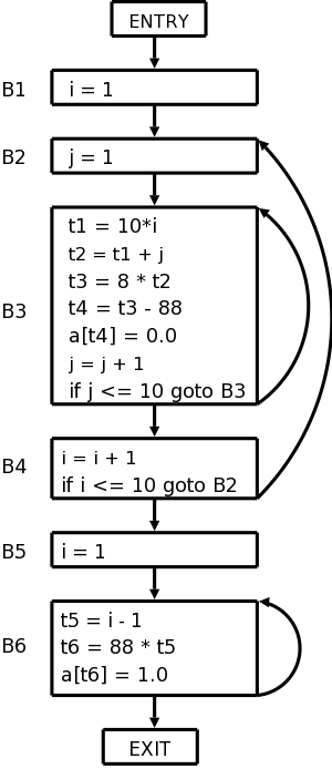
The flow graph for our example is shown on the right.
8.4.4: Representing Flow Graphs
Note that jump targets are no longer quads but blocks.
The reason is that various optimizations within blocks will change
the instructions and we would have to change the jump to reflect
this.
8.4.5: Loops
For most programs the bulk of the execution time is within loops so
we want to identify these.
Definition:
A collection of basic blocks forms a
loop L
with
loop entry E if
- No block in L other than E has a predecessor outside L.
- All blocks in L have a path to E completely inside L.
The flow graph on the right has three loops.
- {B3}, i.e., B3 by itself.
- {B6}.
- {B2, B3, B4}
Homework: 1.
Remark:
Nothing beyond here will be on the final.
A Word or Two About Global Flow Analysis (unofficial)
We are not covering global flow analysis; it is a key component of
optimization and would be a natural topic in a follow-on course.
Nonetheless there is something we can say just by examining the flow
graphs we have constructed.
For this discussion I am ignoring tricky and important
issues concerning arrays and pointer references (specifically,
disambiguation).
You may wish to assume that the program contains no arrays or
pointers for these comments.
We have seen that a simple backwards scan of the statements in a
basic block enables us to determine the variables that are
live-on-entry and those that are dead-on-entry.
Those variables that do not occur in the block are in neither
category; perhaps we should call them ignored by the block
.
We shall see below that it would be lovely to know which variables
are live/dead-on-exit.
This means which variables hold values at the end of the block that
will / will not be used.
To determine the status of v on exit of a block B, we need to trace
all possible execution paths beginning at the end of B.
If all these paths reach a block where v is dead-on-entry before
they reach a block where v is live-on-entry, then v is dead on exit
for block B.
8.5: Optimization of Basic Blocks
8.5.1: The DAG Representation of Basic Blocks
The goal is to obtain a visual picture of how information flows
through the block.
The leaves will show the values entering the block and as we
proceed up the DAG we encounter uses of these values, defs
(and redefs) of values, and uses of the new values.
Formally, this is defined as follows.

- Create a leaf for the initial value of each variable appearing
in the block.
(We do not know what that the value is, not even if the variable
has ever been given a value).
- Create a node N for each statement s in the block.
- Label N with the operator of s.
This label is drawn inside the node.
- Attach to N those variables for which N is the last def in
the block.
These additional labels are drawn along side of N.
- Draw edges from N to each statement that is the last def of
an operand used by N.
- Designate as output nodes those N whose values are
live on exit
, an officially-mysterious term meaning values
possibly used in another block.
(Determining the live on exit values requires global, i.e.,
inter-block, flow analysis.)
As we shall see in the next few sections various basic-block
optimizations are facilitated by using the DAG.
8.5.2: Finding Local Common Subexpressions
As we create nodes for each statement, proceeding in the static
order of the statements, we might notice that a new node is just
like one already in the DAG in which case we don't need a new node
and can use the old node to compute the new value in addition to the
one it already was computing.
Specifically, we do not construct a new node if an existing node
has the same children in the same order and is labeled with the same
operation.
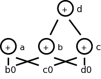
Consider computing the DAG for the following block of code.
    a = b + c
    c = a + x
    d = b + c
    b = a + x
The DAG construction proceeds as follows (the movie on the right
accompanies the explanation).
- First we construct leaves with the initial values.
- Next we process a = b + c.
This produces a node labeled + with a attached and having
b0 and c0 as children.
- Next we process c = a + x.
- Next we process d = b + c.
Although we have already computed b + c in the first statement,
the c's are not the same, so we produce a new node.
- Then we process b = a + x.
Since we have already computed a + x in statement 2, we do not
produce a new node, but instead attach b to the old node.
- Finally, we tidy up and erase the unused initial values.
You might think that with only three computation nodes in the DAG,
the block could be reduced to three statements (dropping the
computation of b).
However, this is wrong.
Only if b is dead on exit can we omit the computation of b.
We can, however, replace the last statement with the simpler
b = c.
Sometimes a combination of techniques finds improvements that no
single technique would find.
For example if a-b is computed, then both a and b are incremented by
one, and then a-b is computed again, it will not be recognized as a
common subexpression even though the value has not changed.
However, when combined with various algebraic transformations, the
common value can be recognized.

8.5.3: Dead Code Elimination
Assume we are told (by global flow analysis) that certain values
are dead on exit.
We examine each root (node with no ancestor) and delete any for
which all attached variables are dead on exit.
This process is repeated since new roots may have appeared.
For example, if we are told, for the picture on the right, that c
and d are dead on exit, then the root d can be removed since d is
dead.
Then the rightmost node becomes a root, which also can be removed
(since c is dead).
8.5.4: The Use of Algebraic Identities
Some of these are quite clear.
We can of course replace x+0 or 0+x by simply x.
Similar considerations apply to 1*x, x*1, x-0, and x/1.
Another class of simplifications is strength reduction,
where we replace one operation by a cheaper one.
A simple example is replacing 2*x by x+x on architectures where
addition is cheaper than multiplication.
A more sophisticated strength reduction is applied by compilers that
recognize induction variables
(loop indices).
Inside a
for i from 1 to N
loop, the expression 4*i can be strength reduced to j=j+4 and 2^i
can be strength reduced to j=2*j (with suitable initializations of j
just before the loop).
Other uses of algebraic identities are possible; many require a
careful reading of the language reference manual to ensure their
legality.
For example, even though it might be advantageous to convert
((a + b) * f(x)) * a
to
((a + b) * a) * f(x)
it is illegal in Fortran since the programmer's use of parentheses
to specify the order of operations can not be violated.
Does
    a = b + c
    x = y + c + b + r
contain a common subexpression of b+c that need be evaluated only
once?
The answer depends on whether the language permits the use of the
associative and commutative law for addition.
(Note that the associative law is invalid for floating point numbers.)
8.5.5: Representation of Array References
Arrays are tricky.
Question: Does
    x = a[i]
    a[j] = 3
    z = a[i]
contain a common subexpression of a[i] that need be evaluated only
once?
The answer depends on whether i=j.
Without some form of disambiguation, we can not be assured that the
values of i and j are distinct.
Thus we must support the worst case condition that i=j and hence the
two evaluations of a[i] must each be performed.
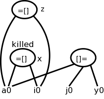
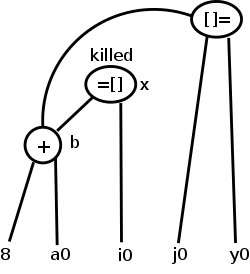
A statement of the form x = a[i] generates a node labeled with the
operator =[] and the variable x, and having children a0,
the initial value of a, and the value of i.

A statement of the form a[j] = y generates a node labeled with
operator []= and three children a0. j, and y, but with no
variable as label.
The new feature is that this node kills all existing nodes depending
on a0.
A killed node can not received any future labels so cannot becomew a
common subexpression.
Returning to our example
    x = a[i]
    a[j] = 3
    z = a[i]
We obtain the top figure to the right.

Sometimes it is not children but grandchildren (or other
descendant) that are arrays.
For example we might have
    b = a + 8    // b[i] is 8 bytes past a[i]
    x = b[i]
    b[j] = y
Again we need to have the third statement kill the second node even
though it is caused by a grandchild.
This is shown in the bottom figure.
8.5.6: Pointer Assignment and Procedure Calls
Pointers are even trickier than arrays.
Together they have spawned a mini-industry in disambiguation
,
i.e., when can we tell whether two array or pointer references refer
to the same or different locations.
A trivial case of disambiguation occurs with.
    p = &x
    *p = y
In this case we know precisely the value of p so the second
statement kills only nodes with x attached.
With no disambiguation information, we must assume
that a pointer can refer to any location.
Consider
    x = *p
    *q = y
We must treat the first statement as a use of every variable;
pictorially the =* operator takes all current nodes with identifiers
as arguments.
This impacts dead code elimination.
We must treat the second statement as writing every variable.
That is all existing nodes are killed, which impacts common
subexpression elimination.
In our basic-block level approach, a procedure call has properties
similar to a pointer reference:
For all x in the scope of P, we must
treat a call of P as using all nodes with x attached and also
kills those same nodes.
8.5.7: Reassembling Basic Blocks From DAGs
Now that we have improved the DAG for a basic block, we need to
regenerate the quads.
That is, we need to obtain the sequence of quads corresponding to
the new DAG.
We need to construct a quad for every node that has a variable
attached.
If there are several variables attached we chose a live-on-exit
variable, assuming we have done the necessary global flow analysis
to determine such variables).
If there are several live-on-exit variables we need to compute one
and make a copy so that we have both.
An optimization pass may eliminate the copy if it is able to assure
that one such variable may be used whenever the other is
referenced.
Example
Recall the example from our movie
    a = b + c
    c = a + x
    d = b + c
    b = a + x
If b is dead on exit, the first three instructions suffice.
If not we produce instead
    a = b + c
    c = a + x
    d = b + c
    b = c
which is still an improvement as the copy instruction is less
expensive than the addition on most architectures.
If global analysis shows that, whenever this definition of b is
used, c contains the same value, we can eliminate the copy and use c
in place of b.
Order of Generated Instructions
Note that of the following 5 rules, 2 are due to arrays, and 2 due
to pointers.
- The DAG order must be respected (defs before uses).
- Assignment to an array must follow all assignments to or uses
of the same array that preceded it in the original block (no
reordering of array assignments).
- Uses of an array must follow all (preceding according to the
original block) assignments to it; so the only transformation
possible is reordering uses.
- All variable references must follow all (preceding ...)
procedure calls or assignment through a pointer.
- A procedure call or assignment through a pointer must follow all
(preceding ...) variable references.
Homework: 9.14,
9.15 (just simplify the 3-address code of 9.14 using the two cases
given in 9.15), and
9.17 (just construct the DAG for the given basic block in the two
cases given).
8.6: A Simple Code Generator
A big issue is proper use of the registers, which are often in
short supply, and which are used/required for several purposes.
- Some operands must be in registers.
- Holding temporaries thereby avoiding expensive memory ops.
- Holding inter-basic-block values (loop index).
- Storage management (e.g., stack pointer).
For this section we assume a RISC architecture.
Specifically, we assume only loads and stores touch memory;
that is, the instruction set consists of
    LD  reg, mem
    ST  mem, reg
    OP  reg, reg, reg
where there is one OP for each operation type used in the three
address code.
A major simplification is we assume that, for each three address
operation, there is precisely one machine instruction that
accomplishes the task.
This eliminates the question of instruction selection.
We do, however, consider register usage.
Although we have not done global flow analysis (part of
optimization), we will point out places where live-on-exit
information would help us make better use of the available registers.
Recall that the mem operand in the load LD and store ST
instructions can use any of the previously discussed addressing
modes.
8.6.1: Register and Address Descriptors
These are the primary data structures used by the code generator.
They keep track of what values are in each register as well as where
a given value resides.
- Each register has a register descriptor containing the
list of variables currently stored in this register.
At the start of the basic block all register descriptors are empty.
- Each variable has a address descriptor containing the
list of locations where this variable is currently stored.
Possibilities are its memory location and one or more registers.
The memory location might be in the static area, the stack, or
presumably the heap (but not mentioned in the text).
The register descriptor could be omitted since you can compute it
from the address descriptors.
8.6.2: The Code-Generation Algorithm
There are basically three parts to (this simple algorithm for) code
generation.
- Choosing registers
- Generating instructions
- Managing descriptors
We will isolate register allocation in a function
getReg(Instruction), which is presented later.
First presented is the algorithm to generate instructions.
This algorithm uses getReg() and the descriptors.
Then we learn how to manage the descriptors and finally we study
getReg() itself.
Machine Instructions for Operations
Given a quad OP x, y, z (i.e., x = y OP z), proceed as follows.
Call getReg(OP x, y, z) to get Rx, Ry, and
Rz, the registers to be used for x, y, and z
respectively.
Note that getReg merely selects the registers, it
does not guarantee that the desired values are present
in these registers.
Check the register descriptor for Ry.
If y is not present in Ry, check the address descriptor
for y and issue
LD Ry, y
The book uses y' (not y) as source of the load, where y'
is some location containing y.
I don't see why just y isn't enough.
Perhaps y might also be in a register, but then I don't see why
Ry wouldn't be that register.
- Similar treatment for Rz.
- Generate the instruction
OP Rx, Ry, Rz
Machine Instructions for Copy Statements
When processing
x = y
steps 1 and 2 are the same as above
(getReg() will set Rx=Ry).
Step 3 is vacuous and step 4 is omitted.
This says that if y was already in a register before the copy
instruction, no code is generated at this point.
Since the value of y is not in its memory location,
we may need to store this value back into y at block exit.
Ending the Basic Block
You probably noticed that we have not yet generated any store
instructions; They occur here (and during spill code in getReg()).
We need to ensure that all variables needed by (dynamically)
subsequent blocks (i.e., those live-on-exit) have their current
values in their memory locations.
- Temporaries are never live beyond a basic block so can be
ignored.
- Variables dead on exit (thank you global flow for determining
such variables) are also ignored.
All live on exit variables (for us all non-temporaries) need
to be in their memory location on exit from the block.
Check the address descriptor for each live on exit variable.
If its own memory location is not listed, generate
ST x, R
where R is a register listed in the address descriptor
Managing Register and Address Descriptors
This is fairly clear.
We just have to think through what happens when we do a load, a
store, an OP, or a copy.
For R a register, let Desc(R) be its register descriptor.
For x a program variable, let Desc(x) be its address descriptor.
- Load: LD R, x
- Desc(R) = x (removing everything else from Desc(R))
- Add R to Desc(x) (leaving alone everything else in Desc(x))
- Remove R from Desc(w) for all w ≠ x
(not in 2e please check)
- Store: ST x, R
- Add the memory location of x to Desc(x)
- Operation: OP Rx, Ry, Rz
implementing the quad OP x, y, z
- Desc(Rx) = x
- Desc(x) = Rx
- Remove Rx from Desc(w) for all w ≠ x
- Copy: For x = y after processing the load (if needed)
- Add x to Desc(Ry) (note y not x)
- Desc(x) = R
Example
Since we haven't specified getReg() yet, we will assume there are
an unlimited number of registers so we do not need to generate any
spill code (saving the register's value in memory).
One of getReg()'s jobs is to generate spill code when a register needs
to be used for another purpose and the current value is not
presently in memory.
Despite having ample registers and thus not generating spill code,
we will not be wasteful of registers.
- When a register holds a temporary value and there are no
subsequent uses of this value, we reuse that register.
- When a register holds the value of a program variable and
there are no subsequent uses of this value, we reuse that
register providing this value is also in the
memory location for the variable.
- When a register holds the value of a program variable and all
subsequent uses of this value are preceded by a redefinition, we
could reuse this register.
But to know about all subsequent uses may require
live/dead-on-exit knowledge.
This example is from the book.
I give another example after presenting getReg(), that I believe
justifies my claim that the book is missing an action, as indicated
above.
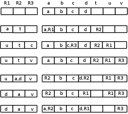
Assume a, b, c, and d are program variables and t, u, v are
compiler generated temporaries (I would call these t$1, t$2, and
t$3).
The intermediate language program is on the left with the generated
code for each quad shown.
To the right is shown the contents of all the descriptors.
The code generation is explained below the diagram.

       t = a - b
           LD  R1, a
           LD  R2, b
           SUB R2, R1, R2


       u = a - c
           LD  r3, c
           SUB R1, R1, R3

       v = t + u
           ADD R3, R2, R1


       a = d
           LD  R2, d


       d = v + u
           ADD R1, R3, R1


       exit
           ST  a, R2
           ST  d, R1
What follows describes the choices made.
Confirm that the values in the descriptors matches the explanations.
- For the first quad, we need all three instructions since nothing
is register resident on block entry.
Since b is not used again, we can reuse its register.
(Note that the current value of b is in its memory location.)
- We do not load a again since its value is R1, which we can reuse
for u since a is not used below.
- We again reuse a register for the result; this time because c is
not used again.
- The copy instruction required a load since d was not in a
register.
As the descriptor shows, a was assigned to the same register, but
no machine instruction was required.
- The last instruction uses values already in registers.
We can reuse R1 since u is a temporary.
- At block exit, lacking global flow analysis, we must assume all
program variables are live and hence must store back to memory any
values located only in registers.
8.6.3: Design of the Function getReg
Consider
x = y OP z
Picking registers for y and z are the same; we just do y.
Choosing a register for x is a little different.
A copy instruction
x = y
is easier.
Choosing Ry
Similar to demand paging, where the goal is to produce an available
frame, our objective here is to produce an available register we can
use for Ry.
We apply the following steps in order until one succeeds.
(Step 2 is a special case of step 3.)
- If Desc(y) contains a register, use of these for Ry.
- If Desc(R) is empty for some registers, pick one of these.
- Pick a register for which the cleaning procedure
generates a minimal number of store instructions.
To clean an in-use register R do the following for each v in Desc(R).
- If Desc(v) includes something besides R, no store is needed
for v.
- If v is x and x is not z, no store is needed since x is
being overwritten.
- No store is needed if there is no further use of v prior to
a redefinition.
This is easy to check for further uses within the block.
If v is live on exit (e.g., we have no global flow analysis),
we need a redefinition later in this block.
- Otherwise a spill ST v, R is generated.
Choosing Rz and Rx, and Processing x = y
As stated above choosing Rz is the same as choosing
Ry.
Choosing Rx has the following differences.
- Since Rx will be written it is not enough for
Desc(x) to contain a register R as in 1. above;
instead, Desc(R) must contain only x.
- If there is no further use of y prior to a redefinition (as
described above for v) and if Ry contains only y (or
will do so after it is loaded), then Ry can be used
for Rx.
Similarly, Rz might be usable for Rx.
getReg(x=y) chooses Ry as above and chooses
Rx=Ry.
Example
                              R1  R2  R3    a    b    c    d    e
  			                  a    b    c    d    e

    a = b + c
        LD  R1, b
        LD  R2, c
        ADD R3, R1, R2
                              R1  R2  R3    a    b    c    d    e
  			    b   c   a     R3  b,R1 c,R2  d    e

    d = a + e
        LD  R1, e
        ADD R2, R3, R1
                              R1  R2  R3    a    b    c    d    e
                       2e →   e   d   a     R3  b,R1  c    R2  e,R1
                       me →   e   d   a     R3   b    c    R2  e,R1
We needed registers for d and e; none were free.
getReg() first chose R2 for d since R2's current contents, the value
of c, was also located in memory.
getReg() then chose R1 for e for the same reason.
Using the 2e algorithm, b might appear to be in R1
(depends if you look in the address or register descriptors).
    a = e + d
        ADD R3, R1, R2
                              Descriptors unchanged

    e = a + b
        ADD R1, R3, R1   ← possible wrong answer from 2e
                              R1  R2  R3    a    b    c    d    e
                              e   d    a    R3  b,R1  c    R2   R1

        LD  R1, b
        ADD R1, R3, R1
                              R1  R2  R3    a    b    c    d    e
                              e   d    a    R3   b    c    R2   R1
The 2e might think R1 has b (address descriptor) and also
conclude R1 has only e (register descriptor) so might generate the
erroneous code shown.
Really b is not in a register so must be loaded.
R3 has the value of a so was already chosen for a.
R2 or R1 could be chosen.
If R2 was chosen, we would need to spill d (we must assume live-on-exit,
since we have no global flow analysis).
We choose R1 since no spill is needed: the value of e (the current
occupant of R1) is also in its memory location.
  exit
      ST  a, R3
      ST  d, R2
      ST  e, R1
8.7: Peephole Optimization
Skipped.
8.8: Register Allocation and Assignment
Skipped.
8.9: Instruction Selection by Tree Rewriting (unofficial)
What if a given quad needs several OPs and we have choices?
We would like to be able to describe the machine OPs in a way that
enables us to find a sequence of OPs (and LDs and STs) to do the job.
The idea is that you express the quad as a tree and express each OP
as a (sub-)tree simplification, i.e. the op replaces a subtree by a
simpler subtree.
In fact the simpler subtree is just a single node.

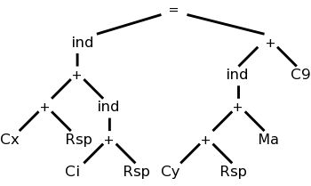
The diagram on the right represents x[i] = y[a] + 9,
where x and y are on the stack and a is in the static area.
M's are values in memory; C's are constants; and R's are registers.
The weird ind (presumably short for indirect) treats its argument as
a memory location.
Compare this to grammars:
A production replaces the RHS by the LHS.
We consider context free grammars where the LHS is a single
nonterminal.
For example, a LD replaces a Memory node with a Register node.
Another example is that
ADD Ri, Ri, Rj
replaces a subtree consisting of a + with both children registers (i
and j) with a Register node (i).
As you do the pattern matching and reductions (apply the
productions), you emit the corresponding code (semantic actions).
So to support a new processor, you need to supply the tree
transformations corresponding to every instruction in the
instruction set.
8.10: Optimal Code Generation for Expressions (unofficial)
This is quite cute.
We assume all operators are binary and label the instruction tree
with something like the height.
This gives the minimum number of registers needed so that no spill
code is required.
A few details follow.
8.10.1: Ershov Numbers
- Draw the
expression tree
, the syntax tree for an expression.
- Label the leaves with 1.
- Label interior nodes with L:
- If the children have the same label x, L=x+1.
This looks like height.
- If the children have different labels, x and y, L=max(x,y).
8.10.2: Generating Code From Labeled Expression Trees
- Recursive algorithm starting at the root.
Each node puts its answer in the highest number register it is
assigned.
The idea is that a node uses (mostly) the same registers as its
sibling.
- If the labels on the children are equal to L, the parent's
label is L+1.
- Give one child L regs ending in highest assigned to
parent.
Note that the lowest reg assigned to the parent is not
used by this child.
The answer appears in top reg assigned to the child, which
is the top reg assigned to the parent.
- Give other child L regs, ending one below the top reg
assigned to the parent.
This child does use the bottom reg assigned to the parent.
The answer appears in top reg assigned to the child, i.e.,
the penultimate parent reg.
- Parent uses a two address OP to compute its answer in the
same reg used by first child, which is the top reg
assigned to the parent.
- If the labels on the children are M<L, the parent is
labeled L.
- Give
bigger
child all L parent regs.
- Give other child M regs ending one below bigger child.
- Parent uses 2-addr OP computing answer in L
- If at a leaf (operand), load it into assigned reg.
Can see this is optimal (assuming you have enough registers).
- Loads each operand only once.
- Performs each operation only once.
- Does no stores.
- Minimal number of registers having the above three properties.
- Show need L registers to produce a result with label L.
- Must compute one side and not use the register containing
its answer before finishing the other side.
- Apply this argument recursively.
8.10.3: Evaluating Expressions with an Insufficient Supply of Registers
Rough idea is to apply the above recursive algorithm, but at each
recursive step, if the number of regs is not enough, store the
result of the first child computed before starting the second.
8.11: Dynamic Programming Code-Generation
Skipped

