Compilers
Start Lecture #2
Statements
Keywords are very helpful for distinguishing statements from one another.
    stmt → id := expr
    	 | if expr then stmt
    	 | if expr then stmt else stmt
    	 | while expr do stmt
    	 | begin opt-stmts end
    opt-stmts → stmt-list | ε
    stmt-list → stmt-list ; stmt | stmt
Remarks:
- In the above example I underlined the non-terminals.
This is not normally done.
It is easy to tell the non-terminals; they are the symbols that
appear on the LHS.
- opt-stmts stands for
optional statements
.
The begin-end block can be empty in some languages.
- The ε (epsilon) stands for the empty string.
- The use of
epsilon productions
will add complications.
- Some languages do not permit empty blocks.
For example, Ada has a
null
statement, which does nothing
when executed and avoids the need for empty blocks.
- The above grammar is ambiguous!
- The notorious
dangling else
problem.
- How do you parse
if x then if y then z=1 else z=2
?
Homework: 4 a-d (for a the operands are digits and the
operators are +, -, *, and /).
2.3: Syntax-Directed Translation
The idea is to specify the translation of a source language
construct in terms of attributes of its syntactic components.
The basic idea is use the productions to specify a (typically
recursive) procedure for translation.
For example, consider the production
stmt-list → stmt-list ; stmt
To process the left stmt-list, we
- Call ourselves recursively to process the right stmt-list
(which is smaller).
This will, say, generate code for all the statements in the
right stmt-list.
- Call the procedure for stmt, generating code for stmt.
- Process the left stmt-list by combining the results for the
first two steps as well as what is needed for the semicolon (a
terminal, so we do not further delegate its actions).
In this case we probably concatenate the code for the right
stmt-list and stmt.
To avoid having to say the right stmt-list
and the left stmt-list
we write the production as
stmt-list → stmt-list1 ; stmt
where the subscript is used to distinguish the two instances of
stmt-list.
Question: Why won't this go on forever?
Answer: Eventually stmt-list1
will consist of only one stmt and then the other
production for stmt-list will be used.

2.3.1: Postfix Notation (an example)
This notation is called postfix because the rule
is operator after operand(s)
.
Parentheses are not needed.
The notation we normally use is called infix.
If you start with an infix expression, the following algorithm will
give you the equivalent postfix expression.
- Variables and constants are left alone.
- E op F becomes E' F' op, where E' and F' are the postfix of E
and F respectively.
- ( E ) becomes E', where E' is the postfix of E.
One question is, given say 1+2-3, what are E, F and op?
Does E=1+2, F=3, and op=-?
Or does E=1, F=2-3 and op=+?
This is the issue of precedence and associativity mentioned above.
To simplify the present discussion we will start with fully
parenthesized infix expressions.
Example: 1+2/3-4*5
- Start with 1+2/3-4*5
- Parenthesize (using standard precedence) to get (1+(2/3))-(4*5)
- Apply the above rules to calculate P{(1+(2/3))-(4*5)}, where
P{X} means
convert the infix expression X to postfix
.
- P{(1+(2/3))-(4*5)}
- P{(1+(2/3))} P{(4*5)} -
- P{1+(2/3)} P{4*5} -
- P{1} P{2/3} + P{4} P{5} * -
- 1 P{2} P{3} / + 4 5 * -
- 1 2 3 / + 4 5 * -
Example: Now do (1+2)/3-4*5
- Parenthesize to get ((1+2)/3)-(4*5)
- Calculate P{((1+2)/3)-(4*5)}
- P{((1+2)/3) P{(4*5)} -
- P{(1+2)/3} P{4*5) -
- P{(1+2)} P{3} / P{4} P{5} * -
- P{1+2} 3 / 4 5 * -
- P{1} P{2} + 3 / 4 5 * -
- 1 2 + 3 / 4 5 * -
2.3.2: Synthesized Attributes
We want to decorate
the parse trees we construct with
annotations
that give the value of certain attributes
of the corresponding node of the tree.
We will do the example of
translating infix to postfix with 1+2/3-4*5.
We use the following grammar, which follows the normal arithmetic
terminology where one multiplies and divides factors to obtain
terms, which in turn are added and subtracted to form expressions.
  expr   → expr + term | expr - term | term
  term   → term * factor | term / factor | factor
  factor → digit | ( expr )
  digit  → 0 | 1 | 2 | 3 | 4 | 5 | 6 | 7 | 8 | 9
This grammar supports parentheses, although our example does not
use them.
On the right is a movie
in which the parse tree is
build from this example.
Question: Was this a top-down or bottom-up movie?
The attribute we will associate with the nodes is the postfix form
of the string in the leaves below the node.
In particular, the value of this attribute at the root is the
postfix form of the entire source.
The book does a simpler grammar (no *, /, or parentheses) for a
simpler example.
You might find that one easier.
Syntax-Directed Definitions (SDDs)
Definition: A syntax-directed definition
is a grammar together with semantic rules associated with
the productions.
These rules are used to compute attribute values.
A parse tree augmented with the attribute values at each node is
called an annotated parse tree.
For the bottom-up approach I will illustrate now, we annotate a
node after having annotated its children.
Thus the attribute values at a node can depend on the children of
the node but not the parent of the node.
We call these synthesized attributes, since they are formed
by synthesizing the attributes of the children.
In chapter 5, when we study top-down annotations as well, we will
introduce inherited
attributes that are passed down from
parents to children.
We specify how to synthesize attributes by giving the semantic
rules together with the grammar.
That is, we give the syntax directed definition.
| Production | Semantic Rule |
|---|
| expr → expr1 + term | expr.t := expr1.t || term.t || '+' |
| expr → expr1 - term | expr.t := expr1.t || term.t || '-' |
| expr → term | expr.t := term.t |
| term → term1 * factor | term.t := term1.t || factor.t || '*'
|
| term → term1 / factor | term.t := term1.t || factor.t || '/'
|
| term → factor | term.t := factor.t |
| factor → digit | factor.t := digit.t |
| factor → ( expr ) | factor.t := expr.t |
| digit → 0 | digit.t := '0' |
| digit → 1 | digit.t := '1' |
| digit → 2 | digit.t := '2' |
| digit → 3 | digit.t := '3' |
| digit → 4 | digit.t := '4' |
| digit → 5 | digit.t := '5' |
| digit → 6 | digit.t := '6' |
| digit → 7 | digit.t := '7' |
| digit → 8 | digit.t := '8' |
| digit → 9 | digit.t := '9' |
We apply these rules bottom-up (starting with the geographically
lowest productions, i.e., the lowest lines in the tree) and get the
annotated graph shown on the right.
The annotation are drawn in green.
Homework: Draw the annotated graph for (1+2)/3-4*5.
2.3.3: Simple Syntax-Directed Definitions
If the semantic rules of a syntax-directed definition all have the
property that the new annotation for the left hand side (LHS) of the
production is just the concatenation of the annotations for the
nonterminals on the RHS in the same order as the nonterminals
appear in the production, we call the syntax-directed
definition simple.
It is still called simple if new strings are interleaved with the
original annotations.
So the example just done is a simple syntax-directed definition.
Remark: SDD's feature semantic rules.
We will soon learn about Translation Schemes, which feature a
related concept called semantic actions.
When one has a simple SDD, the corresponding translation scheme
can be done without constructing the parse tree.
That is, while doing the parse, when you get to the point where you
would construct the node, you just do the actions.
In the translation scheme corresponding to the present example,
the action at a node is just to print the new
strings at the appropriate points.
2.3.4: (depth-first) Tree Traversals
When performing a depth-first tree traversal, it is clear in what
order the leaves are to be visited, namely left to right.
In contrast there are several choices as to when to
visit an interior (i.e. non-leaf) node.
The traversal can visit an interior node
- Before visiting any of its children.
- Between visiting its children.
- After visiting all of its children.
I do not like the book's pseudocode as I feel the names chosen confuse
the traversal with visiting the nodes.
I prefer the pseudocode below, which uses the following conventions.
- Comments are introduced by -- and terminate at the end of the
line (as in the programming language Ada).
- Indenting is significant so begin/end or {} are not used (from
the programming language family B2/ABC/Python)
    traverse (n : treeNode)
        if leaf(n)                      -- visit leaves once; base of recursion
           visit(n)
        else                            -- interior node, at least 1 child
           -- visit(n)                  -- visit node PRE visiting any children
           traverse(first child)        -- recursive call
           while (more children remain) -- excluding first child
               -- visit(n)              -- visit node IN-between visiting children
               traverse (next child)    -- recursive call
           -- visit(n)                  -- visit node POST visiting all children
Note the following properties
- As written, with the last three visit()s commented out, only
the leaves are visited and those visits are in left to right
order.
- If you uncomment just the first (interior node) visit, you get
a preorder traversal, in which each node is visited
before (i.e., pre) visiting any of its children.
- If you uncomment just the last visit, you get a
postorder traversal, in which each node is visited
after (i.e., post) visiting all of its children.
- If you uncomment only the middle visit, you get an
inorder traversal, in which the node is visited (in-)
between visiting its children.
Inorder traversals are normally defined only for binary trees,
i.e., trees in which every interior node has exactly two
children.
Although the code with only the middle visit uncommented
works
for any tree, we will, like everyone else, reserve
the name inorder traversal
for binary trees.
In the case of binary search trees (everything
in the left subtree is smaller than the root of that subtree,
which in tern is smaller than everything in the corresponding
right subtree) an inorder traversal visits the values of the
nodes in (numerical) order.
- If you uncomment two of the three visits, you get a traversal
without a name.
-
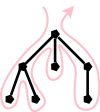 If you uncomment all of the three visits, you get an
Euler-tour traversal.
To explain the name Euler-tour traversal, recall that
an Eulerian tour on a directed graph is one that
traverses each edge once.
If we view the tree on the right as undirected and replace each
edge with two arcs, one in each direction, we see that the pink
curve is indeed an Eulerian tour.
It is easy to see that the curve visits the nodes in the order
of the pseudocode (with all visits uncommented).
Normally, the Euler-tour traversal is defined only for a binary
tree, but this time I will differ from convention and
use the pseudocode above to define Euler-tour traversal for all
trees.
Note the following points about our Euler-tour traversal.
- A node with k children is visited k+1 times.
The diagram shows nodes with 0, 1, 2, and 3 children.
- In a binary tree, a leaf is visited once and an
interior node is visited three times.
This is one of the standard definitions of an Euler-tour
traversal for a binary tree.
- The other standard definition has all nodes visited 3
times.
For a leaf the three visits are in succession.
Modifying the pseudocode to obtain this definition simply
requires replacing the
leaf visit
with
visit(n); visit(n); visit(n)
Remark
In the general case (when not all attributes are synthesized), SDDs
do not impose an evaluation order for the attributes of the parse
tree.
The only requirement is that each attribute is evaluated after all
those that it depends on.
This general case is quite difficult, and sometimes no such order is
possible.
Since, at this point in the course, we are considering only
synthesized attributes, a postorder traversal will always yield a
correct evaluation order for the attributes.
This is so since synthesized attributes depend only on attributes of
child nodes and a postorder traversal visits a node only after all
the children have been visited (and hence all the child node
attributes have been evaluated).
End of Remark.
2.3.5: Translation schemes
The bottom-up annotation scheme just described generates the final
result as the annotation of the root.
In our infix to postfix example we get the result desired by
printing the root annotation.
Now we consider another technique that produces its results
incrementally.
Instead of giving semantic rules for each production (and thereby
generating annotations) we can embed program fragments
called semantic actions within the productions themselves.
When drawn in diagrams (e.g., see the diagram below), the semantic
action is connected to its node with a distinctive, often dotted,
line.
The placement of the actions determine the order they are performed.
Specifically, one executes the actions in the order they are
encountered in a depth-first traversal of the tree (the children of
a node are visited in left to right order).
Note that these action nodes are all leaves and hence they are
encountered in the same order for both preorder and postorder
traversals (and inorder and Euler-tree order).
Definition: A
syntax-directed translation scheme is a context-free
grammar with embedded semantic actions.
In the SDD for our infix to postfix translator, the parent
either
- takes the attribute of its only child or
- concatenates the attributes left to right of its several
children and adds something at the end.
The equivalent semantic actions is to either print nothing or
print the new item.
Emitting a Translation
Here are the semantic actions corresponding to a few of the rows of
the table above.
Note that the actions are enclosed in {}.
| Production with Semantic Action
| Semantic Rule
|
|
|
| expr → expr1 + term
| { print('+') }
| expr.t := expr1.t || term.t || '+'
|
| expr → expr1 - term
| { print('-') }
| expr.t := expr1.t || term.t || '-'
|
| term → term1 / factor
| { print('/') }
| term.t := term1.t || factor.t || '/'
|
| term → factor
| { null }
| term.t := factor.t
|
| digit → 3
| { print ('3') }
| digit.t := '3'
|

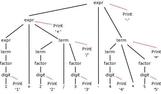
The diagram for 1+2/3-4*5 with attached semantic actions is shown
on the right.
Given an input, e.g. our favorite 1+2/3-4*5, we just do a
(left-to-right) depth first traversal of the corresponding diagram
and perform the semantic actions as they occur.
When these actions are print statements as above, we are said to be
emitting the translation.
Do on the board a depth first traversal of the diagram, performing
the semantic actions as they occur, and confirm that the translation
emitted is in fact 123/+45*-, the postfix version of 1+2/3-4*5
Homework: Produce the corresponding diagram for
(1+2)/3-4*5.
Prefix to infix translation
When we produced postfix, all the prints came at the end (so that
the children were already printed
).
The { action }'s do not need to come at the end.
We illustrate this by producing infix arithmetic (ordinary) notation
from a prefix source.

In prefix notation the operator comes first.
For example, +1-23 evaluates to zero and +-123 evaluates to 2.
Consider the following grammar, which generates the simple language
of prefix expressions consisting of addition and subtraction of
digits between 1 and 3 without parentheses (prefix notation and
postfix notation do not use parentheses).
P → + P P | - P P | 1 | 2 | 3
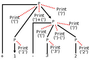
The resulting parse tree for +1-23 with the semantic actions
attached is shown on the right.
Note that the output language (infix notation) has
parentheses.
The table below shows both the semantic actions and rules used by
the translator.
Normally, one does not use both actions and rules.
I do it here so that we can compare them and see how closely related
they are.
Prefix to infix translator
| Production with Semantic Action | Semantic Rule
|
|
|
| P → + { print('(') } P1 { print(')+(') }
P2 { print(')') }
| P.t := '(' || P1.t || ')+(' || P.t || ')'
|
|
|
| P → - { print('(') } P1 { print(')-(') }
P2 { print(')') }
| P.t := '(' || P1.t || ')-(' || P.t || ')'
|
|
|
| P → 1 { print('1') } | P.t := '1' |
|
|
| P → 2 { print('2') } | P.t := '2' |
|
|
| P → 3 { print('3') } | P.t := '3' |
First do a preorder traversal of the tree and see that you get
1+(2-3).
In fact you don't get that answer, but instead get a fully
parenthesized version that is equivalent.
Next start a postorder traversal and see that it produces the
same output (i.e., executes the same prints in the same order).
Question: What about an Euler-tour order?
Answer: The same result.
For all traversals, the leaves are printed in left
to right order and all the semantic actions are leaves.
Finally, pretend the prints aren't there, i.e., consider
the unannotated parse tree and perform
a postorder traversal, evaluating the semantic
rules at each node encountered.
Postorder is needed (and sufficient) since we have
synthesized attributes and hence having child attributes evaluated
prior to evaluating parent attributes is both necessary and
sufficient to ensure that whenever an attribute is evaluated all the
component attributes have already been evaluated.
(It will not be so easy in chapter 5, when we have inherited
attributes as well.)
Homework: 2.
2.4: Parsing
Objective: Given a string of tokens and a grammar, produce a
parse tree yielding that string (or at least determine if such a
tree exists).
We will learn both top-down (begin with the start symbol, i.e. the
root of the tree) and bottom up (begin with the leaves) techniques.
In the remainder of this chapter we just do top down, which is
easier to implement by hand, but is less general.
Chapter 4 covers both approaches.
Tools (so called parser generators
) often use bottom-up
techniques.
In this section we assume that the lexical analyzer has already
scanned the source input and converted it into a sequence of tokens.

2.4.1: Top-down parsing
Consider the following simple language, which derives a subset
of the types found in the (now somewhat dated) programming language
Pascal.
I do not assume you know pascal.
We have two nonterminals, type, which is the start symbol, and
simple, which represents the simple
types.
There are 8 terminals, which are tokens produced by the lexer and
correspond closely with constructs in pascal itself.
Specifically, we have.
- integer and char
- id for identifier
- array and of used in array declarations
- ↑ meaning pointer to
- num for a (positive whole) number
- dotdot for .. (used to give a range like 6..9)
The productions are
    type   → simple
    type   → ↑ id
    type   → array [ simple ] of type
    simple → integer
    simple → char
    simple → num dotdot num
Parsing is easy in principle and for certain grammars (e.g., the
one above) it actually is easy.
We start at the root since this is top-down parsing and apply
the two fundamental steps.
- At the current (nonterminal) node, select a production whose LHS
is this nonterminal and whose RHS
matches
the input at this
point.
Make the RHS the children of this node (one child per RHS symbol).
- Go to the next node needing a subtree.
When programmed this becomes a procedure for each nonterminal that
chooses a production for the node and calls procedures for each
nonterminal in the RHS of that production.
Thus it is recursive in nature and descends the parse tree.
We call these parsers recursive descent
.
The big problem is what to do if the current node is the LHS of
more than one production.
The small problem is what do we mean by the next
node needing
a subtree.
The movie on the right, which succeeds in parsing, works by tossing
2 ounces of pixie dust into the air and choosing the production onto
which the most dust falls.
(An alternative interpretation is given below.)
The easiest solution to the big problem would be to assume that
there is only one production having a given terminal as LHS.
There are two possibilities
- No circularity. For example
    expr → term + term - 9
    term → factor / factor
    factor → digit
    digit → 7
But this is very boring. The only possible sentence
is 7/7+7/7-9
- Circularity
    expr → term + term
    term → factor / factor
    factor → ( expr )
This is even worse; there are no (finite) sentences. Only an
infinite sentence beginning (((((((((.
So this won't work.
We need to have multiple productions with the same LHS.
How about trying them all?
We could do this!
If we get stuck where the current tree cannot match the input we are
trying to parse, we would backtrack.
Instead, we will look ahead one token in the input and only choose
productions that can yield a result starting with this token.
Furthermore, we will (in this section) restrict ourselves to
predictive parsing in which there is only one production
that can yield a result starting with a given token.
This solution to the big problem also solves the small problem.
Since we are trying to match the next token in the input, we must
choose the leftmost (nonterminal) node to give children to.
2.4.2: Predictive parsing
Let's return to pascal array type grammar and consider the three
productions having type as LHS.
Remember that, even when I write the short form
type → simple | ↑ id | array [ simple ] of type
we still have three productions.
For each production P we wish to consider the set FIRST(P)
consisting of those tokens (i.e., terminals) that can appear as the
first symbol of a string derived from the RHS of P.
FIRST is actually defined on strings not productions.
When I write FIRST(P), I really mean FIRST(RHS).
Similarly, I often say
the first set of the production P
when I should really say
the first set of the RHS of the production P
.
Formally, we proceed as follows.
Let α be a string of terminals and/or non-terminals.
FIRST(α) is the set of terminals that can appear as
the first symbol in a string of terminals derived from α.
If α is ε or α can derive ε, then
ε is in FIRST(α)
So given α we find all strings of terminals that can be
derived from α and pick off the first terminal.
Definition: Let r be the RHS of a production P.
FIRST(P) is FIRST(r).
To use predictive parsing, we make the following
Assumption: Let P and Q be two productions with
the same LHS,
Then FIRST(P) and FIRST(Q) are disjoint.
Thus, if we know both the LHS and the token that must be first, there
is (at most) one production we can apply.
BINGO!
An example of predictive parsing
This table gives the FIRST sets for our pascal array type example.
| Production | FIRST |
|---|
| type → simple | { integer, char, num } |
| type → ↑ id | { ↑ } |
| type → array [ simple ] of type | { array } |
| simple → integer | { integer } |
| simple → char | { char } |
| simple → num dotdot num | { num } |
Make sure that you understand how this table was
derived.
It is not yet clear how to calculate FIRST for a complicated
example.
We will learn the general procedure in chapter 4.
Note that the three productions with type as LHS have disjoint
FIRST sets.
Similarly the three productions with simple as LHS have disjoint
FIRST sets.
Thus predictive parsing can be used.
We process the input left to
right and call the current token lookahead since it is how
far we are looking ahead in the input to determine the production to
use.
The movie on the right shows the process in action.
Homework:
A. Construct the FIRST sets for
  rest → + term rest | - term rest | term
  term → 1 | 2 | 3
B. Can predictive parsing be used?
End of Homework.

2.4.3: When to Use ε-productions
Not all grammars are as friendly as the last example. The first
complication is when ε occurs as a RHS. If this happens or
if the RHS can generate ε, then ε is included in
FIRST.
But ε would always match the current input position!
The rule is that if lookahead is not in FIRST of any production
with the desired LHS, we use the (unique!) production (with that
LHS) that has ε as RHS.
The text does a C instead of a pascal example.
The productions are
    stmt → expr ;
         | if ( expr ) stmt
         | for ( optexpr ; optexpr ; optexpr ) stmt
         | other
 optexpr → expr | ε
For completeness, on the right is the beginning of a
movie for the C example.
Note the use of the ε-production at the end since no other
entry in FIRST will match ;
Once again, the full story will be revealed in chapter 4 when we do
parsing in a more complete manner.
2.4.4: Designing a Predictive Parser
Predictive parsers are fairly easy to construct as we will now see.
Since they are recursive descent parsers we go top-down with one
procedure for each nonterminal.
Do remember that to use predictive parsing, we must have disjoint
FIRST sets for all the productions having a given nonterminal as
LHS.
- For each nonterminal, write a procedure that chooses the
unique(!) production having lookahead in its FIRST set.
Use the ε production if no other production matches.
If no production matches and there is no ε production, the
parse fails.
- These procedures mimic the RHS of the production.
They call procedures for each nonterminal and call match for each
terminal.
- Write a procedure match(terminal) that advances lookahead to
the next input token after confirming that the previous value of
lookahead equals the terminal argument.
- Write a main program that initializes lookahead to the first input
token and invokes the procedure for the start symbol.
The book has code at this point, which you should read.
 If you uncomment all of the three visits, you get an
Euler-tour traversal.
