Start Lecture #13
Skipped.
Our intermediate code uses symbolic labels.
At some point these must be translated into addresses of
instructions.
If we use quads all instructions are the same length so the address
is just the number of the instruction.
Sometimes we generate the jump before we generate the target so we
can't put in the instruction number on the fly
.
Indeed, that is why we used symbolic labels.
The easiest method of fixing this up is to make an extra pass (or
two) over the quads to determine the correct instruction number and
use that to replace the symbolic label.
This is extra work; a more efficient technique, which is independent
of compilation, is called backpatching
.
Evaluate an expression, compare it with a vector of constants that are viewed as labels of the arms of the switch, and execute the matching arm (or a default).
The C language is unusual in that the various cases are just labels
for a giant computed goto
at the beginning.
The more traditional idea is that you execute just one of the arms,
as in a series of
      if
      else if
      else if
      ...
      end if
else if'sabove. This executes roughly k jumps (worst case) for k cases.
The lab 3 grammar does not have a switch statement so we won't do a detailed SDD.
An SDD for the second method above could be organized as follows.
Much of the work for procedures involves storage issues and the run time environment; this is discussed in the next chapter.
In order to support inter-procedural type checking using just one pass over the SDD we need to define the called procedure for use by the calling procedure. The lab3 grammar is not quite capable of this for the general case.
When a procedure (or function) definition is parsed, we could place in the outermost identifier table the signature of the procedure (defined below).
Then when the call is reached the types can be checked. So all is well if the callee precedes the caller, which would be a requirement with the lab3 grammar (this is not strictly true, one could gather up the program while going through the tree and then at the root make a function call—a synthesized attribute—to a procedure that just happens to be another compiler that can handle this case). The requirement that callee precedes caller eliminates the important case of mutual recursion where f calls g and g calls f.
We will not produce SDDs for the special case that can be handled by our grammar.
The basic scheme for type checking procedures is to
generate a table entry for the procedure that contains
its signature
, i.e., the types of its parameters and its
result type.
Recall the SDD
for declarations.
These semantic rules pass up the totalSize to the
ds → d ds
production.
What is needed is for the ps (parameters) to do an analogous thing with their declarations but also (or perhaps instead) pass up a representation of the declarations themselves which when it reaches the top is the signature for a procedure and when put together with the return is the signature for a function.
More serious is supporting nested procedure definitions (defining a procedure inside a procedure). Lab 3 doesn't support this because a procedure or function definition is not a declaration. It would be easy to enhance the grammar to fix this, but the serious work is that then you need nested identifier tables.
Since our lexer doesn't support this, the parser must produce the nested tables (using the tables that the lexer does generate). When a new scope (procedure definition, record definition, begin block) arises you push the current tables on a stack and begin a new one. When the nested scope ends, you pop the tables.
Homework: Read Chapter 7.
We are discussing storage organization from the point of view of the compiler, which must allocate space for programs to be run. In particular, we are concerned with only virtual addresses and treat them uniformly.
This should be compared with an operating systems treatment, where we worry about how to effectively map this configuration to real memory. For example see these two diagrams in my OS class notes, which illustrate an OS difficulty with our allocation method, which uses a very large virtual address range. Perhaps the most straightforward solution uses multilevel page tables.
Some system require various alignment constraints. For example 4-byte integers might need to begin at a byte address that is a multiple of four. Unaligned data might be illegal or might lower performance. To achieve proper alignment padding is often used.
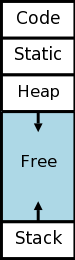
expansion region.
new, or via a library function call, such as malloc(). It is deallocated either by another executable statement, such as a call to free(), or automatically by the system.
Much (often most) data cannot be statically allocated. Either its size is not known at compile time or its lifetime is only a subset of the program's execution.
Early versions of Fortran used only statically allocated data. This required that each array had a constant size specified in the program. Another consequence of supporting only static allocation was that recursion was forbidden (otherwise the compiler could not tell how many versions of a variable would be needed).
Modern languages, including newer versions of Fortran, support both static and dynamic allocation of memory.
The advantage supporting dynamic storage allocation is the increased flexibility and storage efficiency possible (instead of declaring an array to have a size adequate for the largest data set; just allocate what is needed). The advantage of static storage allocation is that it avoids the runtime costs for allocation/deallocation and may permit faster code sequences for referencing the data.
An (unfortunately, all too common) error is a so-called memory leak
where a long running program repeated allocates memory that it fails
to delete, even after it can no longer be referenced.
To avoid memory leaks and ease programming, several programming
language systems employ automatic garbage collection
.
That means the runtime system itself determines when data
can no longer be referenced and automatically deallocates it.
Achievements.
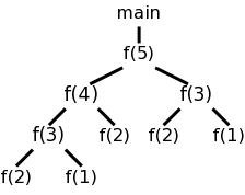
Recall the fibonacci sequence 1,1,2,3,5,8, ... defined by f(1)=f(2)=1 and, for n>2, f(n)=f(n-1)+f(n-2). Consider the function calls that result from a main program calling f(5). Surrounding the more-general pseudocode that calculates (very inefficiently) the first 10 fibonacci numbers, we show the calls and returns that result from main calling f(5). On the left they are shown in a linear fashion and, on the right, we show them in tree form. The latter is sometimes called the activation tree or call tree.
    System starts main
        enter f(5)
            enter f(4)
                enter f(3)
		    enter f(2)
		    exit f(2)
		    enter f(1)
		    exit f(1)
                exit f(3)
                enter f(2)	       int a[10];
                exit f(2)	       int main(){
            exit f(4)		           int i;
            enter f(3)		           for (i=0; i<10; i++){
	        enter f(2)	               a[i] = f(i);
		exit f(2)	           }
		enter f(1)	       }
		exit f(1)	       int f (int n) {
            exit f(3)		           if (n<3)  return 1;
        exit f(5)		           return f(n-1)+f(n-2);
    main ends			       }
We can make the following observation about these procedure calls.
The information needed for each invocation of a procedure is kept in a runtime data structure called an activation record (AR) or frame. The frames are kept in a stack called the control stack.
Note that this is memory used by the compiled program, not by the compiler. The compiler's job is to generate code that obtains the needed memory.
At any point in time the number of frames on the stack is the current depth of procedure calls. For example, in the fibonacci execution shown above when f(4) is active there are three activation records on the control stack.
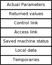
ARs vary with the language and compiler implementation. Typical components are described below and pictured to the right. In the diagrams the stack grows down the page.
actual parameters). The first few arguments are often placed in registers.

The diagram on the right shows (part of) the control stack for the fibonacci example at three points during the execution. In the upper left we have the initial state, We show the global variable a, although it is not in an activation record and actually is allocated before the program begins execution (it is statically allocated; recall that the stack and heap are each dynamically allocated). Also shown is the activation record for main, which contains storage for the local variable i.
Below the initial state we see the next state when main has called f(1) and there are two activation records, one for main and one for f. The activation record for f contains space for the argument n and and also for the result. There are no local variables in f.
At the far right is a later state in the execution when f(4) has been called by main and has in turn called f(2). There are three activation records, one for main and two for f. It is these multiple activations for f that permits the recursive execution. There are two locations for n and two for the result.
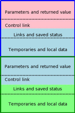
The calling sequence, executed when one procedure (the caller) calls another (the callee), allocates an activation record (AR) on the stack and fills in the fields. Part of this work is done by the caller; the remainder by the callee. Although the work is shared, the AR is called the callee's AR.
Since the procedure being called is defined in one place, but normally called from many places, we would expect to find more instances of the caller activation code than of the callee activation code. Thus it is wise, all else being equal, to assign as much of the work to the callee as possible.
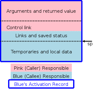
The top picture illustrates the situation where a pink procedure (the caller) calls a blue procedure (the callee). Also shown is Blue's AR. Note that responsibility for this single AR is shared by both procedures. The picture is just an approximation: For example, the returned value is actually Blue's responsibility, although the space might well be allocated by Pink. Also some of the saved status, e.g., the old sp, is saved by Pink.
The bottom picture shows what happens when Blue, the callee, itself
calls a green procedure and thus Blue is also a caller.
You can see that Blue's responsibility includes part of its AR as
well as part of Green's.
Note that varagrs are supported.
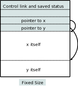
There are two flavors of variable-length data.
It is the second flavor that we wish to allocate on the stack. The goal is for the (called) procedure to be able to access these arrays using addresses determinable at compile time even though the size of the arrays (and hence the location of all but the first element) is not known until the program is called, and indeed often differs from one call to the next (even when the two calls correspond to the same source statement.
The solution is to leave room for pointers to the arrays in the AR. These are fixed size and can thus be accessed using static offsets. Then when the procedure is invoked and the sizes are known, the pointers are filled in and the space allocated.
A small change caused by storing these variable size items on the stack is that it no longer is obvious where the real top of the stack is located relative to sp. Consequently another pointer (call it real-top-of-stack) is also kept. This is used on a call to tell where the new allocation record should begin.
As we shall see the ability of procedure p to access data declared outside of p (either declared globally outside of all procedures or declared inside another procedure q) offers interesting challenges.
In languages like standard C without nested procedures, visible names are either local to the procedure in question or are declared globally.
With nested procedures a complication arises. Say g is nested inside f. So g can refer to names declared in f. These names refer to objects in the AR for f; the difficulty is finding that AR when g is executing. We can't tell at compile time where the (most recent) AR for f will be relative to the current AR for g since a dynamically-determined (i.e., statically unknown) number of routines could have been called in the middle.
There is an example in the next section. in which g refers to x, which is declared in the immediately outer scope (main) but the AR is 2 away because f was invoked in between. (In that example you can tell at compile time what was called in what order, but with a more complicated program having data-dependent branches, it is not possible.)
The book asserts (correctly) that C doesn't have nested procedures so introduces ML, which does (and is quite slick), but which many of you don't know and I haven't used. Fortunately, a common extension to C is to permit nested procedures. In particular, gcc supports nested procedures. To check my memory I compiled and ran the following program.
  #include <stdio.h>

  int main (int argc, char *argv[])
  {
  int x = 10;

  int g(int y)
  {
  int z = x+3;
  return z;
  }

  int f (int y)
  {
  return g(y)+1;
  }

  printf("The answer is %d\n", f(x));
  return 0;
  }
The program compiles without errors and the correct answer of 14 is printed.
So we can use C (really the GCC extension of C).
Remark: Many consider this gcc extension to be evil.
Outermost procedures have nesting depth 1. Other procedures have nesting depth 1 more than the nesting depth of the immediately outer procedure. In the example above main has nesting depth 1; both f and g have nesting depth 2.
The AR for a nested procedure contains an access link that points to the AR of the most recent activation of the immediately outer procedure).
So in the example above the access link for f and g would point to the AR of the activation of main. Then when f references x, defined in main, the activation record for main can be found by following the access link in the AR for f. Since f is nested in main, they are compiled together so, once the AR is determined, the same techniques can be used as for variables local to f.
This example was too easy.
However the technique is quite general. For a procedure P to access a name defined in the 3-outer scope (i.e., the unique outer scope whose nesting depth is 3 less than that of P; make sure you understand why an outer scope is unique), you follow the access links three times.
The question is how are the access links maintained.
Let's assume there are no procedure parameters. We are also assuming that the entire program is compiled at once.
Without procedure parameters, the compiler knows the name of the called procedure and the nesting depth.
Let the caller be procedure R (the last letter in caller) and let the called procedure be D. Let N(f) be the nesting depth of f.
	P() {
          D() {...}
          P1() {
            P2() {
              ...
              Pk() {
                R(){... D(); ...}
              }
             ...
            }
          }
        }
Our goal while creating the AR for D at the call from R is to set
the access link to point to the AR for P.
Note that this entire structure in the skeleton code shown is
visible to the compiler.
Thus, the current (at the time of the call) AR is the one for R
and if we follow the access links k+1 times we get a pointer to
the AR for P, which we can then place in the access link for the
being-created AR for D.
The above works fine when R is nested (possibly deeply) inside D. It is the picture above but P1 is D.
When k=0 we get the gcc code I showed before and also the case of direct recursion where D=R. I do not know why the book separates out the case k=0, especially since the previous edition didn't.
Skipped. The problem is that, if f calls g with a parameter of h (or a pointer to h in C-speak) and the g calls this parameter (i.e., calls h), g might not know the context of h. The solution is for f to pass to g the pair (h, the access link of h) instead of just passing h. Naturally, this is done by the compiler, the programmer is unaware of access links.
Basically skipped. In theory access links can form long chains (in practice, nesting depth rarely exceeds a dozen or so). A display is an array in which entry i points to the most recent (highest on the stack) AR of depth i.
Almost all of this section is covered in the OS class.
Covered in OS.
Covered in Architecture.
Covered in OS.
Covered in OS.
Stack data is automatically deallocated when the defining procedure returns. What should we do with heap data explicated allocated with new/malloc?
The manual method is to require that the programmer explicitly deallocate these data. Two problems arise.
	loop
	allocate X
	use X
	forget to deallocate X
As this program continues to run it will require more and more
storage even though is actual usage is not increasing
significantly.
	allocate X
	use X
	deallocate X
	100,000 lines of code not using X
	use X
Both can be disastrous.
The system detects data that cannot be accessed (no direct or indirect references exist) and deallocates the data automatically.
Covered in programming languages.
Skipped
Skipped.
Skipped.
Skipped.
Skipped.
Skipped.
Skipped.
Skipped.
Skipped.
Skipped.
Skipped.
Skipped.
Skipped.
Skipped.
Skipped.
Skipped.
Skipped
Skipped.
Skipped.
Skipped.
Skipped.
Homework: Read Chapter 8.
Goal: Transform intermediate code + tables into final machine (or assembly) code. Code generation + Optimization is the back end of the compoiler.
As expected the input to the code generator is the output of the intermediate code generator. We assume that all syntactic and semantic error checks have been done by the front end. Also, all needed type conversions are already done and any type errors have been detected.
We are using three address instructions for our intermediate language. These instructions have several representations, quads, triples, indirect triples, etc. In this chapter I will tend to use the term quad (for brevity) when I should really say three-address instruction, since the representation doesn't matter.
A RISC (Reduced Instruction Set Computer), e.g. PowerPC, Sparc, MIPS (popular for embedded systems), is characterized by
Onlyloads and stores touch memory
A CISC (Complex Instruct Set Computer), e.g. x86, x86-64/amd64 is characterized by
A stack-based computer is characterized by
Noregisters
IBM 701/704/709/7090/7094 (Moon shot, MIT CTSS) were accumulator based.
Stack based machines were believed to be good compiler targets. They became very unpopular when it was believed that register architecture would perform better. Better compilation (code generation) techniques appeared that could take advantage of the multiple registers.
Pascal P-code and Java byte-code are the machine instructions for a hypothetical stack-based machine, the JVM (Java Virtual Machine) in the case of Java. This code can be interpreted, or compiled to native code.
RISC became all the rage in the 1980s.
CISC made a gigantic comeback in the 90s with the intel pentium
pro.
A key idea of the pentium pro is that the hardware would
dynamically translate a complex x86 instruction into a series of
simpler RISC-like
instructions called ROPs (RISC ops).
The actual execution engine dealt with ROPs.
The jargon would be that, while the architecture (the ISA) remained
the x86, the micro-architecture was quite different and more like
the micro-architecture seen in previous RISC processors.
For maximum compilation speed, the compiler accepts the entire
program at once and produces code that can be loaded and executed
(the compilation system can include a simple loader and can start
the compiled program).
This was popular for student jobs
when computer time was
expensive.
The alternative, where each procedure can be compiled separately,
requires a linkage editor.
It eases the compiler's task to produce assembly code instead of machine code and we will do so. This decision increased the total compilation time since it requires an extra assembler pass (or two).
A big question is the level of code quality we seek to attain.
For example can we simply translate one quadruple at a time.
The quad
x = y + z
can always (assuming x, y, and z are statically allocated, i.e.,
their address is a compile time constant off the sp) be compiled
into
    LD  R0, y
    ADD R0, R0, z
    ST  x, R0
But if we apply this to each quad separately (i.e., as a separate.
problem) then
    LD  R0, b
    ADD R0, R0, c
    ST  a, R0
    LD  R0, a
    ADD R0, e
    ST  d, R0
The fourth statement is clearly not needed since we are loading into
R0 the same value that it contains.
The inefficiency is caused by our compiling the second quad with no
knowledge of how we compiled the first quad.
Since registers are the fastest memory in the computer, the ideal solution is to store all values in registers. However, there are normally not nearly enough registers for this to be possible. So we must choose which values are in the registers at any given time.
Actually this problem has two parts.
The reason for the second problem is that often there are register requirements, e.g., floating-point values in floating-point registers and certain requirements for even-odd register pairs (e.g., 0&1 but not 1&2) for multiplication/division.
Sometimes better code results if the quads are reordered. One example occurs with modern processors that can execute multiple instructions concurrently, providing certain restrictions are met (the obvious one is that the input operands must already be evaluated).