Compilers

Start Lecture #10

6.1.2: The Value-Number Method for Constructing DAGS

Often one stores the tree or DAG in an array, one entry per node. Then the array index, rather than a pointer, is used to reference a node. This index is called the node's value-number and the triple
    <op, value-number of left, value-number of right>
is called the signature of the node. When Node(op,left,right) needs to determine if an identical node exists, it simply searches the table for an entry with the required signature.

Searching an unordered array is slow; there are many better data structures to use. Hash tables are a good choice.

Homework: 2.

6.2: Three-Address Code

Instructions of the form op a,b,c, where op is a primitive operator. For example

    lshift a,b,4   // left shift b by 4 and place result in a
    add    a,b,c   // a = b + c
    a = b + c      // alternate (more natural) representation of above
  

If we are starting with a DAG (or syntax tree if less aggressive), then transforming into 3-address code is just a topological sort and an assignment of a 3-address operation with a new name for the result to each interior node (the leaves already have names and values).

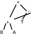
For example, (B+A)*(Y-(B+A)) produces the DAG on the right, which yields the following 3-address code.

    t1 = B + A
    t2 = Y - t1
    t3 = t1 * t2
  

6.2.1: Addresses and Instructions

We use the term 3-address since instructions in our intermediate-code consist of one elementary operation with three operands, each of which is an address. Typically two of the addresses represent source operands or arguments of the operation and the third represents the result. Some of the 3-address operations have fewer than three addresses; we simply think of the missing addresses as unused (or ignored) fields in the instruction.

Possible addresses

1. (Source program) Names. Really the intermediate code would contain a reference to the (identifier) table entry for the name. For convenience, the actual identifier is often written.
2. Constants. Again, this would often be a reference to a table entry. An important issue is type conversion that will be discussed later. Type conversion also applies to identifiers.
3. (Compiler-generated) Temporaries. Although it may at first seem wasteful, modern practice assigns a new name to each temporary, rather than reusing the same temporary. (Remember that a DAG node is considered one temporary even if it has many parents.) Later phases can combine several temporaries into one (e.g., if they have disjoint lifetimes).

Possible three-address instructions

There is no universally agreed to set of three-address instructions or to whether 3-address code should be the intermediate code for the compiler. Some prefer a set close to a machine architecture. Others prefer a higher-level set closer to the source, for example, subsets of C have been used. Others prefer to have multiple levels of intermediate code in the compiler and define a compilation phase that converts the high-level intermediate code into the low-level intermediate code. What follows is the set proposed in the book.

In the list below, x, y, and z are addresses; i is an integer, not an address); and L is a symbolic label. The instructions can be thought of as numbered and the labels can be converted to the numbers with another pass over the output or via backpatching, which is discussed below.

1. Binary and unary ops.
   1. x = y op z, a binary op
   2. x = op y, a unary op,
   3. x = y, a unary op (in this case the identity f(x)=x)
   
   
2. Binary, unary, and nullary op jumps
   1. Nullary Junp.
      goto L
   2. Conditional unary op jumps.
      if x goto L
      ifFalse x goto L.
   3. Conditional binary op jumps.
      if x relop y goto L
   
   
3. Procedure/Function Calls and Returns.
         param x     call p,n     y = call p,n     return     return y.
   The value n gives the number of parameters, which is needed when the argument of one function is the value returned by another, for example A = F(S,G(U,V),W) might become

   	param S
   	param U
   	param V
   	t = call G,2
   	param t
   	param W
   	A = call F,3
         

4. Indexed Copy ops. x = y[i]   x[i] = y.
   x[i] is the address that is the-value-of-i locations after x; in particular x[0] is the same address as x. Similarly for y[i].

   Note that x[i] = y[j] is not permitted as that requires 4 addresses. x[i] = y[i] could be permitted, but is not.
   
   

5. Address and pointer ops. x = &y   x = *y   *x = y.
   x = &y sets the r-value of x equal to the l-value of y.
   x = *y sets the r-value of x equal to the contents of the location given by the r-value of y.
   *x = y sets the location given by the r-value of x equal to the r-value of y.

6.2.2: Quadruples (Quads)

An easy way to represent the three address instructions: put the op into the first of four fields and the addresses into the remaining three. Some instructions do not use all the fields. Many operands will be references to entries in tables (e.g., the identifier table).

6.2.3: (Indirect) Triples

Triples

A triple optimizes a quad by eliminating the result field of a quad since the result is often a temporary.

When this result occurs as a source operand of a subsequent instruction, the source operand is written as the value-number of the instruction yielding this result (distinguished some way, say with parens).

If the result field of a quad is not a temporary then two triples may be needed:

1. Do the operation and place the result into a temporary (which is not a field of this instruction).
2. A copy instruction from the temporary to the final home. Recall that a copy does not use all the fields of a quad so fits into a triple without omitting the result.

Indirect Triples

When an optimizing compiler reorders instructions for increased performance, extra work is needed with triples since the instruction numbers, which have changed, are used implicitly. Hence the triples must be regenerated with correct numbers as operands.

With Indirect triples we maintain an array of pointers to triples and, if it is necessary to reorder instructions, just reorder these pointers. This has two advantages.

1. The pointers are (probably) smaller than the triples so faster to move. This is a generic advantage and could be used for quads and many other reordering applications (e.g., sorting large records).
2. Since the triples don't move, the references they contain to past results remain accurate. This advantage is specific to triples (or similar situations).

Homework: 1, 2 (you may use the parse tree instead of the syntax tree if you prefer).

6.3: Types and Declarations

Much of the early part of this section is really programming languages.

6.3.1: Type Expressions

A type expression is either a basic type or the result of applying a type constructor.

6.3.2: Type Equivalence

There are two camps, name equivalence and structural equivalence.

Consider the following for example.

    declare
       type MyInteger is new Integer;
       MyX : MyInteger;
       x   : Integer := 0;
    begin
       MyX := x;
    end
  

As another example, consider an object of an anonymous type as in
      X : array [5] of integer;
X does not have the same type as any other object not even Y declared as
      y : array [5] of integer;
However, x[2] has the same type as y[3]; both are integers.

6.3.3: Declarations

The following example from the 2ed uses C/Java array notation. (The 1ed had pascal-like notation.) Although I prefer Ada-like constructs as in lab 3, I realize that the class knows C/Java best so like the authors I will sometimes follow the 2ed as well as presenting lab3-like grammars.

The grammar below gives C/Java like records/structs/methodless-classes as well as multidimensional arrays (really arrays of arrays).

    D → T id ; D | ε
    T → B C | RECORD { D }
    B → INT | FLOAT
    C → [ NUM ] C | ε
  

The lab 3 grammar doesn't support records. Here is a part of the lab3 grammar that handles declarations of ints, reals and arrays.

    declarations         → declaration declarations | ε
    declaration          → defining-identifier : type ; |
                           TYPE defining-identifier IS type ;
    defining-identifier  → IDENTIFIER
    type                 → INT | REAL | ARRAY [ NUMBER ] OF type
  

    ds   → d ds | ε
    d    → di : t ;
    di   → ID
    t    → INT | REAL | ARRAY [ NUMBER ] OF t
  

6.3.4: Storage Layout for Local Names

We are considering here only those types for which the storage requirements can be computed at compile time. For others, e.g., string variables, dynamic arrays, etc, we would only be reserving space for a pointer to the structure; the structure itself would be created at run time. Such structures are discussed in the next chapter.

The idea (for arrays whose size can be determined at compile time) is that the basic type determines the width of the data, and the size of an array determines the height. These are then multiplied to get the size (area) of the data.

The book uses semantic actions (i.e., a syntax directed translation SDT). I added the corresponding semantic rules so that we have an SDD as well. in both case cases we just show a single declaration (i.e., the start symbol is T not D).

Remember that for an SDT, the placement of the actions withing the production is important. Since it aids reading to have the actions lined up in a column, we sometimes write the production itself on multiple lines. For example the production T→BC in the table below has the B and C on separate lines so that (the first two) actions can be in between even though they are written to the right. These two actions are performed after the B child has been traversed, but before the C child has been traversed. The final two actions are at the very end so are done after both children have been traversed.

The actions use global variables t and w to carry the base type (INT or FLOAT) and width down to the ε-production, where they are then sent on their way up and become multiplied by the various dimensions. In the rules I use inherited attributes bt and bw for the same purpose.. This is similar to the comment above that instead of having the identifier table passed up and down via attributes, the bullet can be bitten and a globally visible table used instead.

The base types and widths are set by the lexer or are constants in the parser.

Using the Lab 3 Grammar

This is easier with the lab3 grammar since there are no inherited attributes. We again assume that the lexer has defined NUM.value (it is likely a field in the numbers table entry for the token NUM). The goal is to augment the identifier table entry for ID to include the type and size information found in the declaration. This can be written two ways.

1. addType(ID.entry,t.type)
   addSize(ID.entry,t.size)
2. ID.entry.type=t.type
   ID.entry.size=t.size

Remark: Our lab3 grammar also has type declarations; that is, you can declare that an identifier is a type and can then declare objects of that type.

6.3.5: Sequences of Declarations

The Run Time Storage of Objects

Be careful to distinguish between three methods used to store and pass information.

1. Atrributes. These are variables in a phase (semantics analyzer; also intermediate code generator) of the compiler.
2. Identifier (and other) table. This is longer lived data; often passed between phases.
3. Run time storage. This is storage established by the compiler, but not used by the compiler. It is allocated and used during run time.

To summarize, the identifier table (and others we have used) are not present when the program is run. But there must be run time storage for objects. We need to know the address each object will have during execution. Specifically, we need to know its offset from the start of the area used for object storage.

For just one object, it is trivial: the offset is zero.

Multiple Declarations

The goal is to permit multiple declarations in the same procedure (or program or function). For C/java like languages this can occur in two ways.

1. Multiple objects in a single declaration.
2. Multiple declarations in a single procedure.

In either case we need to associate with each object being declared the location in which it will be stored at run time. Specifically we include in the table entry for the object, its offset from the beginning of the current procedure. We initialize this offset at the beginning of the procedure and increment it after each object declaration.

The lab3 grammar does not support multiple objects in a single declaration.

C/Java does permit multiple objects in a single declaration, but surprisingly the 2e grammar does not.

Naturally, the way to permit multiple declarations is to have a list of declarations in the natural right-recursive way. The 2e C/Java grammar has D which is a list of semicolon-separated T ID's
    D → T ID ; D | ε

The lab 3 grammar has a list of declarations (each of which ends in a semicolon). Shortening declarations to ds we have
    ds → d ds | ε

As mentioned, we need to maintain an offset, the next storage location to be used by an object declaration. The 2e snippet below introduces a nonterminal P for program that gives a convenient place to initialize offset.

    P →                { offset = 0; }
        D
    D → T ID ;         { top.put(id.lexeme, T.type, offset);
                              offset = offset + T.width; }
        D1
    D → ε
  

The name top is used to signify that we work with the top symbol table (when we have nested scopes for record definitions we need a stack of symbol tables). Top.put places the identifier into this table with its type and storage location. We then bump offset for the next variable or next declaration.

Rather than figure out how to put this snippet together with the previous 2e code that handled arrays, we will just present the snippets and put everything together on the lab 3 grammar.

In the function-def (fd) and procedure-def (pd) productions we add the inherited attribute offset to declarations (ds.offset) and set it to zero. We then inherit this offset down to an individual declaration. If this is an object declaration, we store it in the entry for the identifier being declared and we increment the offset by the size of this object. When we get the to the end of the declarations (the ε-production), the offset value is the total size needed. So we turn it around and send it back up the tree.

Now show what happens when the following program is parsed and the semantic rules above are applied.

    procedure test () is
        y : integer;
        x : array [10] of real;
    begin
        y = 5;        // we haven't yet done statements
        x[2] = y;     // type error?
    end;
  

6.3.6: Fields in Records and Classes

Since records can essentially have a bunch of declarations inside, we only need add
T → RECORD { D }
to get the syntax right. For the semantics we need to push the environment and offset onto stacks since the namespace inside a record is distinct from that on the outside. The width of the record itself is the final value of (the inner) offset.

    T → record {         { Env.push(top);  top = new Env()
                           Stack.puch(offset); offset = 0; }
    D }                  { T.type = record(top); T.width = offset;
                           top = Env.pop(); offset = Stack.pop(); }
  

This does not apply directly to the lab 3 grammar since the grammar does not have records. It does, however, have procedures that can be nested.

Actually it does not; we would need some more syntax. To have nested procedures, we would need to add another alternative to declaration: a procedure/function definition. Similarly if we wanted to have nested blocks we would add another alternative to statement.

    s           → ks | is | block-stmt
    block-stmt  → DECLARE ds BEGIN ss END ;
  

If we wanted to generate code for nested procedures or nested blocks, we would need to stack the symbol table as done above and in the text.

Homework: 1.