Compilers

Start Lecture #3

An example of predictive parsing

This table gives the FIRST sets for our pascal array type example.

Make sure that you understand how this table was derived.

Note that the three productions with type as LHS have disjoint FIRST sets. Similarly the three productions with simple as LHS have disjoint FIRST sets. Thus predictive parsing can be used. We process the input left to right and call the current token lookahead since it is how far we are looking ahead in the input to determine the production to use. The movie on the right shows the process in action.

Homework:

A. Construct the corresponding table for

  rest → + term rest | - term rest | term
  term → 1 | 2 | 3

End of Homework.

2.4.3: When to Use ε-productions

Not all grammars are as friendly as the last example. The first complication is when ε occurs as a RHS. If this happens or if the RHS can generate ε, then ε is included in FIRST.

But ε would always match the current input position!

The rule is that if lookahead is not in FIRST of any production with the desired LHS, we use the (unique!) production (with that LHS) that has ε as RHS.

The text does a C instead of a pascal example. The productions are

    stmt → expr ;
         | if ( expr ) stmt
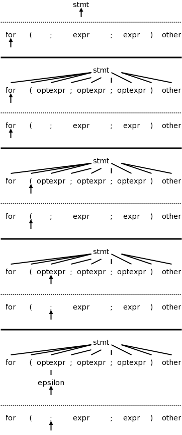
         | for ( optexpr ; optexpr ; optexpr ) stmt
         | other
 optexpr → expr | ε
  

For completeness, on the right is the beginning of a movie for the C example. Note the use of the ε-production at the end since no other entry in FIRST will match ;

Once again, the full story will be revealed in chapter 4 when we do parsing in a more complete manner.

2.4.4: Designing a Predictive Parser

Predictive parsers are fairly easy to construct as we will now see. Since they are recursive descent parsers we go top-down with one procedure for each nonterminal. Do remember that to use predictive parsing, we must have disjoint FIRST sets for all the productions having a given nonterminal as LHS.

1. For each nonterminal, write a procedure that chooses the unique(!) production having lookahead in its FIRST set. Use the ε production if no other production matches. If no production matches and there is no ε production, the parse fails.
2. These procedures mimic the RHS of the production. They call procedures for each nonterminal and call match for each terminal.
3. Write a procedure match(terminal) that advances lookahead to the next input token after confirming that the previous value of lookahead equals the terminal argument.
4. Write a main program that initializes lookahead to the first input token and invokes the procedure for the start symbol.

The book has code at this point, which you should read.

2.4.5: Left Recursion

Another complication. Consider
    expr → expr + term
    expr → term

For the first production the RHS begins with the LHS. This is called left recursion. If a recursive descent parser would pick this production, the result would be that the next node to consider is again expr and the lookahead has not changed. An infinite loop occurs. (Also note that the first sets are not disjoint.)

Note that this is NOT a problem with the grammar per se, but is a limitation of predictive parsing. For example if we had the additional production
    term → x
Then there is no problem finding a parse tree for
    x x
but we won't find it with predictive parsing.

If we tried
expr → term + expr
expr → term
the result would be right recursive, which is no problem. But the first sets are not disjoint.

Consider instead
expr → term rest
rest → + term rest
rest → ε

Both sets of productions generate the same possible token strings, namely
term + term + ... + term
The second set is called right recursive since the RHS ends (has on the right) the LHS. If you draw the parse trees generated, you will see that, for left recursive productions, the tree grows to the left; whereas, for right recursive, it grows to the right.

This will, a month or so from now make it harder for us to get left associativity for arithmetic, but we shall succeed!

In general, for any nonterminal A, and any strings α, and β, we can replace the pair
A → A α | β
with the triple
A → β R
R → α R | ε
where R is a nonterminal not equal to A and not appearing in α or β, i.e., R is a new nonterminal.

For the example above A is expr, R is rest, α is + term, and β is term.

2.5: A Translator for Simple Expressions

Objective: an infix to postfix translator for expressions. We start with just plus and minus, specifically the expressions generated by the following grammar. We include a set of semantic actions with the grammar. Note that finding a grammar for the desired language is one problem, constructing a translator for the language, given a grammar, is another problem. We are tackling the second problem.

  expr → expr + term { print('+') }
  expr → expr - term { print('-') }
  expr → term
  term → 0           { print('0') }
  . . .
  term → 9           { print('9') }

One problem that we must solve is that this grammar is left recursive.

2.5.1: Abstract and concrete syntax

We prefer not to have superfluous nonterminals as they make the parsing less efficient. That is why we don't say that a term produces a digit and a digit produces each of 0,...,9. Ideally the syntax tree would just have the operators + and - and the 10 digits 0,1,...,9. That would be called the abstract syntax tree. A parse tree coming from a grammar is technically called a concrete syntax tree.

2.5.2: Adapting the Translation Scheme

We eliminate the left recursion as we did in 2.4. This time there are two operators + and - so we replace the triple
A → A α | A β | γ
with the quadruple
A → γ R
R → α R | β R | ε

This time we have actions so, for example
α is + term { print('+') }
However, the formulas still hold and we get

  expr → term rest
  rest → + term { print('+') } rest
       | - term { print('-') } rest
       | ε
  term → 0           { print('0') }
       . . .
       | 9           { print('9') }

2.5.3: Procedures for the nonterminals expr, term, and rest

The C code is in the book. Note the else ; in rest(). This corresponds to the epsilon production. As mentioned previously. The epsilon production is only used when all others fail (that is why it is the else arm and not the then or the else if arms).

2.5.4: Simplifying the translator

These are (useful) programming techniques.

The complete program

The program in Java is in the book.

2.6: Lexical analysis

Converts a sequence of characters (the source) into a sequence of tokens. A lexeme is the sequence of characters comprising a single token. The reason we were able to produce the translator in the previous section without a lexer is that all the tokens were just one character (that is why we had just single digits).

2.6.1: Removal of White space and comments

These do not become tokens so that the parser need not worry about them.

2.6.2: Reading ahead

Consider distinguishing x<y from x<=y.

After reading the < we must read another character. If it is a y, we have found our token (<). However, we must unread the y so that when asked for the next token we will start at y. If it is never more than one extra character that must be examined, a single char variable would suffice. A more general solution is discussed in the next chapter (Lexical Analysis).

2.6.3: Constants

This chapter considers only numerical integer constants. They are computed one digit at a time by value=10*value+digit. The parser will therefore receive the token num rather than a sequence of digits. Recall that our previous parsers considered only one digit numbers.

The value of the constant can be considered the attribute of the token named num. Alternatively, the attribute can be a pointer/index into the symbol table entry for the number (or into a numbers table).

2.6.4: Recognizing identifiers and keywords

The C statement
sum = sum + x;
contains 6 tokens. The scanner will convert the input into
id = id + id ; (id standing for identifier).
Although there are three id tokens, the first and second represent the lexeme sum; the third represents x. These must be distinguished. Many language keywords, for example then, are syntactically the same as identifiers. These also must be distinguished. The symbol table will accomplish these tasks. We assume (as do most modern languages) that the keywords are reserved, i.e., cannot be used as program variables. The we simply initialize the symbol table to contain all these reserved words and mark them as keywords. When the lexer encounters a would-be identifier and searches the symbol table, it finds out that the string is actually a keyword.

Care must be taken when one lexeme is a proper subset of another. Consider
x<y versus x<=y
When the < is read, the scanner needs to read another character to see if it is an =. But if that second character is y, the current token is < and the y must be pushed back onto the input stream so that the configuration is the same after scanning < as it is after scanning <=.

Also consider then versus thenewvalue, one is a keyword and the other an id.

2.6.5: A lexical analyzer

A Java program is given. The book, but not the course, seems to assume knowledge of Java.

Since the scanner converts digits into num's we can shorten the grammar. Here is the shortened version before the elimination of left recursion. Note that the value attribute of a num is its numerical value.

    expr   → expr + term    { print('+') }
    expr   → expr - term    { print('-') }
    expr   → term
    term   → num            { print(num.value) }
  

    expr   → expr + term    { print('+') }
    expr   → expr - term    { print('-') }
    expr   → term
    term   → factor
    factor → ( expr ) | num { print(num,value) }
  

The factor() procedure follows the familiar recursive descent pattern: Find a production with factor as LHS and lookahead in FIRST, then do what the RHS says. That is call the procedures corresponding to the nonterminals, match the terminals, and execute the semantic actions

2.7: Incorporating a symbol table

The symbol table is an important data structure for the entire compiler. One example of its use would be for semantic actions associated with declarations to set the type field of an entry; semantic actions associated with expression evaluation would used this type information. For the simple infix to postfix translator (which is typeless), the table is primarily used to store and retrieve <lexeme,token> pairs.

2.7.1: Symbol Table per Scope

There is a serious issue here involving scope. We will learn soon that lexers are based on regular expressions; whereas parsers are based on the stronger but more expensive context-free grammars. Regular expressions are not powerful enough to handle nested scopes. So, if the language you are compiling supports nested scopes, the lexer can only construct the <lexeme,token> pairs. The parser converts these pairs into a true symbol table that reflects the nested scopes. If the language is flat, the scanner can produce the symbol table.

The idea is that, when entering a block, a new symbol table is created. Each such table points to the one immediately outer. This structure supports the most-closely nested rule for symbols: a symbol is in the scope of most-closely nested declaration. This gives rise to a tree of tables.

Interface

• Create table: A new table is created and points to the immediately outer table, which is passed as a argument.
• Insert entry (in the current table).
• Retrieve entry (from the most-closely nested table in which it appears.

Reserved keywords

Simply insert them into the symbol table prior to examining any input. Then they can be found when used correctly and, since their corresponding token will not be id, any use of them where an identifier is required can be flagged. For example one would have insert(int) performed for every table.

2.7.2: The Use of Symbol Tables

Below is the grammar for a stripped down example showing nested scopes. The language consists just of declarations of the form
    identifier : type ; -- I like ada not C style declarations
trivial statements of the form
    identifier ;
and nested blocks.

  program → block
  block   → { decls stmts }     -- { } are terminals not actions
  decls   →  decls decl | ε     -- study this one
  decl    → id : type ;
  stmts   → stmts stmt | ε      -- same idea, a list
  stmt    → block | factor ;    -- get nested block
  factor  → id

One possible program in this language is

    { x : int ;   y : float ;
      x ;   y ;
      {  x : float ;
         x ;   y ;
      }
      {  y : int ;
         x ;   y;
      }
      x ;   y ;
    }
  

To show that we have correctly parsed the input and obtained its meaning (i.e., performed semantic analysis), we present a translation scheme that digests the declarations and translates the statements so that we get

  { int ; float ;   { float ; float ; }   { int ; int ; } }
  

The translation scheme, slightly modified from the book page 90, is shown on the right. First a formatting comment.

This translation scheme looks weird, but is actually a good idea (of the authors): it reconciles the two goals of respecting the ordering and nonetheless having the actions all in one column.

Recall that the placement of the actions within the RHS of the production is significant. The parse tree with its actions is processed in a depth first manner so that the actions are performed in left to right order. Thus an action is executed after all the subtrees rooted by parts of the RHS to the left of the action and is executed before all the subtrees rooted by parts of the RHS to the right of the action.

Consider the first production. We want the action to be executed before processing block. Thus the action must precede block in the RHS. But we want the actions in the right column. So we split the RHS over several lines and place an action in the rightmost column of the line that puts in the right order.

The second production has some semantic actions to be performed at the start of the block, and others to be performed at the bottom.

To fully understand the details, you must read the book; but we can see how it works. A new Env initializes a new symbol table; top.put inserts into the symbol table in the environment top; top.get retrieves from that symbol table.

In some sense the star of the show is the simple production
factor → id
together with its semantic actions. These actions look up the identifier in the (correct!) symbol table and print out the type name.

2.8: Intermediate Code Generation

2.8.1: Two kinds of Intermediate Representations

There are two important forms of intermediate representations.

• Trees, especially parse trees and syntax trees.
• Linear, especially three-address code

    while-stmt → while ( expr ) stmt ;
  

    new While(x,y)
  

    stmt  → block          { stmt.n = block.n }
    block → { stmts }      { block.n = stmts.n }
  

    while ( x == 5 ) {
       blah
       blah
       more
    }
  

    ADD        x y z
    MULT       a b c
    ARRAY_L    q r s
    ARRAY_R    e f g
    ifTrueGoto x L
    COPY       r s
  

    x = y + z
    a = b * c
    q[r] = s
    e = f[g]
    ifTrue x goto L
    r = s
  

    class If extends Stmt {
       Expr E; Stmt S;
       public If(Expr x, Stmt y) { E = x;  S = y;  after = newlabel(); }
       public void gen() {
          Expr n = E.rvalue();
          emit ("ifFalse" + n.toString() + "goto " + after);
          S.gen();
          emit(after + ":");
       }
    }
  

    Expr rvalue(x : Expr) {
       if (x is an Id or Constant node) return x;
       else if (x is an Op(op, y, z) node) {
	  t = new temporary;
	  emit string for t = rvalue(y) op rvalue(z);
	  return a new node for t;
       else read book for other cases
  

We saw in this movie an example where parsing got stuck because we reduced the wrong part of the input string. We also learned about FIRST sets that enabled us to determine which production to apply when we are operating left to right on the input. For predictive parsers the FIRST sets for a given nonterminal are disjoint and so we know which production to apply. In general the FIRST sets might not be disjoint so we have to try all the productions whose FIRST set contains the lookahead symbol.

All the above assumed that the input was error free, i.e. that the source was a sentence in the language. What should we do when the input is erroneous and we get to a point where no production can be applied?

In many cases this is up to the parser to detect/repair. Sometimes the lexer is stuck because there are no patterns that match the input at this point.

The simplest solution is to abort the compilation stating that the program is wrong, perhaps giving the line number and location where the lexer and/or parser could not proceed.

We would like to do better and at least find other errors. We could perhaps skip input up to a point where we can begin anew (e.g. after a statement ending semicolon), or perhaps make a small change to the input around lookahead so that we can proceed.

3.2: Input Buffering

Determining the next lexeme often requires reading the input beyond the end of that lexeme. For example, to determine the end of an identifier normally requires reading the first whitespace character after it. Also just reading > does not determine the lexeme as it could also be >=. When you determine the current lexeme, the characters you read beyond it may need to be read again to determine the next lexeme.

3.2.1: Buffer Pairs

The book illustrates the standard programming technique of using two (sizable) buffers to solve this problem.

3.2.2: Sentinels

A useful programming improvement to combine testing for the end of a buffer with determining the character read.

3.3: Specification of Tokens

The chapter turns formal and, in some sense, the course begins. The book is fairly careful about finite vs infinite sets and also uses (without a definition!) the notion of a countable set. (A countable set is either a finite set or one whose elements can be put into one to one correspondence with the positive integers. That is, it is a set whose elements can be counted. The set of rational numbers, i.e., fractions in lowest terms, is countable; the set of real numbers is uncountable, because it is strictly bigger, i.e., it cannot be counted.) We should be careful to distinguish the empty set φ from the empty string ε. Formal language theory is a beautiful subject, but I shall suppress my urge to do it right and try to go easy on the formalism.

3.3.1: Strings and Languages

We will need a bunch of definitions.

Definition: An alphabet is a finite set of symbols.

Example: {0,1}, presumably φ (uninteresting), ascii, unicode, ebcdic, latin-1.

Definition: A string over an alphabet is a finite sequence of symbols from that alphabet. Strings are often called words or sentences.

Example: Strings over {0,1}: ε, 0, 1, 111010. Strings over ascii: ε, sysy, the string consisting of 3 blanks.

Definition: The length of a string is the number of symbols (counting duplicates) in the string.

Example: The length of allan, written |allan|, is 5.

Definition: A language over an alphabet is a countable set of strings over the alphabet.

Example: All grammatical English sentences with five, eight, or twelve words is a language over ascii. It is also a language over unicode.

Definition: The concatenation of strings s and t is the string formed by appending the string t to s. It is written st.

Example: εs = sε = s for any string s.

We view concatenation as a product (see Monoid in wikipedia http://en.wikipedia.org/wiki/Monoid). It is thus natural to define s⁰=ε and sⁱ⁺¹=sⁱs.

Example: s¹=s, s⁴=ssss.

More string terminology

A prefix of a string is a portion starting from the beginning and a suffix is a portion ending at the end. More formally,

Definitions:

1. A prefix of s is any string obtained from s by removing (possibly zero) characters from the end of s.
2. A suffix is defined analogously.
3. A substring of s is obtained by deleting a prefix and a suffix.

Note: Any prefix or suffix is a substring.

Examplex: If s is 123abc, then
(1) s itself and ε are each a prefix, suffix, and a substring.
(2) 12 are 123a are prefixes and substrings.
(3) 3abc is a suffix and a substring.
(4) 23a is a substring.

Definitions: A proper prefix of s is a prefix of s other than ε and s itself. Similarly, proper suffixes and proper substrings of s do not include ε and s.

Definition: A subsequence of s is formed by deleting (possibly zero) positions from s. We say positions rather than characters since s may for example contain 5 occurrences of the character Q and we only want to delete a certain 3 of them.

Example: issssii is a subsequence of Mississippi.

Note: Any substring is a subsequence.

Homework: 3(a,b,c).

3.3.2: Operations on Languages

Definition: The union of L1 and L2, written L ∪ M is simply the set-theoretic union, i.e., it consists of all words (strings) in either L1 or L2.

Example: Let the alphabet be ascii. The union of {Grammatical English sentences with one, three, or five words} with {Grammatical English sentences with two or four words} is {Grammatical English sentences with five or fewer words}.

Definition: The concatenation of L1 and L2 is the set of all strings st, where s is a string of L1 and t is a string of L2.

We again view concatenation as a product and write LM for the concatenation of L and M.

Examples:: The concatenation of {a,b,c} and {1,2} is {a1,a2,b1,b2,c1,c2}. The concatenation of {aa,b,c} and {1,2,ε} is {aa1,aa2,aa,b1,b2,b,c1,c2,c}.

Definition: As with strings, it is natural to define powers of a language L.
L⁰={ε}, which is not φ.
Lⁱ⁺¹=LⁱL.

Definition: The (Kleene) closure of L, denoted L^* is
L⁰ ∪ L¹ ∪ L² ...

Definition: The positive closure of L, denoted L⁺ is
L¹ ∪ L² ...

Example: {0,1,2,3,4,5,6,7,8,9}⁺ gives all unsigned integers, but with some ugly versions. It has 3, 03, 000003.
{0} ∪ ( {1,2,3,4,5,6,7,8,9} ({0,1,2,3,4,5,6,7,8,9}^* ) ) seems better.

In these notes I may write * for ^* and + for ⁺, but that is strictly speaking wrong and I will not do it on the board or on exams or on lab assignments.

Example: {a,b}* is {ε,a,b,aa,ab,ba,bb,aaa,aab,aba,abb,baa,bab,bba,bbb,...}.
{a,b}+ is {a,b,aa,ab,ba,bb,aaa,aab,aba,abb,baa,bab,bba,bbb,...}.
{ε,a,b}* is {ε,a,b,aa,ab,ba,bb,...}.
{ε,a,b}+ is the same as {ε,a,b}*.

The book gives other examples based on L={letters} and D={digits}, which you should read..

3.3.3: Regular Expressions

The idea is that the regular expressions over an alphabet consist of
the alphabet, and expressions using union, concatenation, and *,
but it takes more words to say it right. For example, I didn't include (). Note that (A ∪ B)* is definitely not A* ∪ B* (* does not distribute over ∪) so we need the parentheses.

The book's definition includes many () and is more complicated than I think is necessary. However, it has the crucial advantages of being correct and precise.

The wikipedia entry doesn't seem to be as precise.

I will try a slightly different approach, but note again that there is nothing wrong with the book's approach (which appears in both first and second editions, essentially unchanged).

Definition: The regular expressions and associated languages over an alphabet consist of

1. ε, the empty string; the associated language L(ε) is {ε}.
2. Each symbol x in the alphabet; L(x) is {x}.
3. rs for all regular expressions (REs) r and s; L(rs) is L(r)L(s).
4. r|s for all REs r and s; L(r|s) is L(r) ∪ L(s).
5. r* for all REs r; L(r*) is (L(r))*.
6. (r) for all REs r; L((r)) is L(r).

Parentheses, if present, control the order of operations. Without parentheses the following precedence rules apply.

The postfix unary operator * has the highest precedence. The book mentions that it is left associative. (I don't see how a postfix unary operator can be right associative or how a prefix unary operator such as unary - could be left associative.)

Concatenation has the second highest precedence and is left associative.

| has the lowest precedence and is left associative.

The book gives various algebraic laws (e.g., associativity) concerning these operators.

The reason we don't include the positive closure is that for any RE
r⁺ = rr^*.

Homework: 2(a-d), 4.

3.3.4: Regular Definitions

These look like the productions of a context free grammar we saw previously, but there are differences. Let Σ be an alphabet, then a regular definition is a sequence of definitions

  d1 → r1
  d2 → r2
      ...
  dn → rn

Note that each d_i can depend on all the previous d's.

Note also that each d_i can not depend on following d's. This is an important difference between regular definitions and productions (the latter are more powerful).

Example: C identifiers can be described by the following regular definition

  letter_ → A | B | ... | Z | a | b | ... | z | _
    digit → 0 | 1 | ... | 9
      CId → letter_ ( letter_ | digit)*

Regular definitions are just a convenience; they add no power to regular expressions. The C identifier example can be done simply as a regular expression by simply plugging in the earlier definitions to the later ones.

3.3.5: Extensions of Regular Expressions

There are many extensions of the basic regular expressions given above. The following three will be occasionally used in this course as they are useful for lexical analyzers.

All three are simply shorthand. That is, the set of possible languages generated using the extensions is the same as the set of possible languages generated without using the extensions.

1. One or more instances. This is the positive closure operator + mentioned above.
2. Zero or one instance. The unary postfix operator ? defined by
   r? = r | ε for any RE r.
3. Character classes. If a₁, a₂, ..., a_n are symbols in the alphabet, then
   [a₁a₂...a_n] = a₁ | a₂ | ... | a_n. In the special case where all the a's are consecutive, we can simplify the notation further to just [a₁-a_n].