Compilers

Remark: Lab3 assigned: (top-down) parser. The first non-programming part, is due in 7 days. The other two parts due in 21 days (2 NYU weeks).

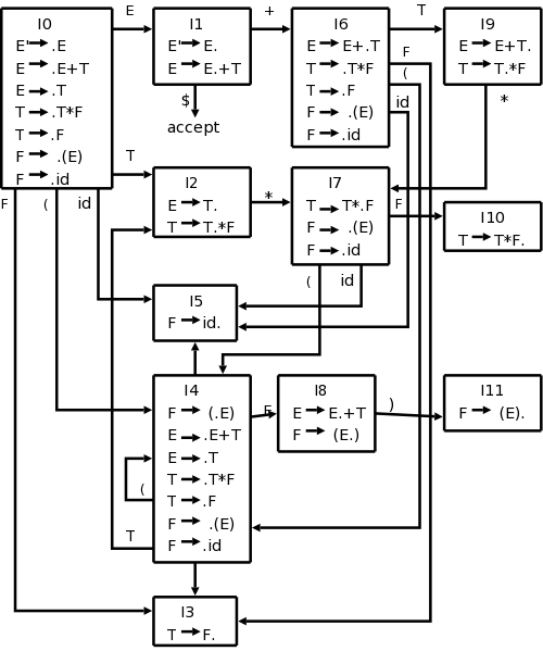
I₀, I₁, etc are called (LR(0)) item sets, and the collection with the arcs (i.e., the DFA) is called the LR(0) automaton.

Stack	Symbols	Input	Action
$0		id+id$	Shift to 3
$03	id	+id$	Reduce by T→id
$02	T	+id$	Reduce by E→T.
$01	E	+id$	Shift to 4
$014	E+	id$	Shift to 3
$0143	E+id	$	Reduce by T→id
$0145	E+T	$	Reduce by E→E+T
$01	E	$	Accept

Now we put the diagram to use to parse id+id as shown in the table on the right. The symbols column is not needed since it can be determined from the stack, but it is useful for understanding.

We start in the initial state with the stack empty and the input full. The $'s are just end markers. From state 0, called I0 in my diagram (following the book they are called I's since they are sets of items), we can only shift in the id (the nonterminals will appear in the symbols column). This brings us to I3 so we push a 3 onto the stack

In I3 we first notice that there is no outgoing arc labeled with a terminal; hence we cannot do a shift. However, we do see a completed production in the box (the dot is on the extreme right). That means we have seen (i.e., shifted) in the input the entire RHS of a production. Thus we can reduce by this production. To reduce we pop the stack for each symbol in the RHS since we are replacing the RHS by the LHS. This time the RHS has one symbol so we pop the stack once and also remove one symbol from the symbols column. The stack corresponds to moves so we are undoing the move to 3 and we are temporarily in 0 again. But the production has a T on the LHS so we follow the T production from 0 to 2, push T onto Symbols, and push 2 onto the stack.

In I2 we again see no possible shift but do see a completed production and do another reduction, which brings us to 1.

You might think that at I1 we could reduce using the completed bottom production, but that is wrong. This (E→E·) item is special and can only be applied when we are at the end of the input string.

Thus the next two steps are shifts of + and id, sending us to 3 again, where, as before, we have no choice but to reduce the id to T and are in step 5 ready for the big one.

The reduction in 5 has three symbols on the RHS so we pop (back up) three times again temporarily landing in 0, but the RHS puts us in 1.

Perfect! We have just E as a symbol and the input is empty so we are ready to reduce by E'→E, which signifies acceptance.

Now we rejoin the book and say it more formally.

Actually there is more than mere formality coming. For the example above, we had no choices, but that was because the example was simple. We need more machinery to insure that we never have two or more possible moves to choose among.

Closure of Item Sets

Say I is a set of items and one of these items is A→α·Bβ. This item represents the parser having seen α and records that the parser might soon see the remainder of the RHS. For that to happen the parser must first see a string derivable from B. Now consider any production starting with B, say B→γ. If the parser is to make progress on A→α·Bβ, it will need to be making progress on one such B→·γ. Hence we want to add all the latter productions to any state that contains the former. We formalize this into the notion of closure.

Definition: For any set of items I, CLOSURE(I) is formed as follows.

1. Initialize CLOSURE(I) = I
2. If A → α · B β is in CLOSURE(I) and B → γ is a production, then add B → · γ to the closure and repeat.

Example: Recall our main example

   E' → E
    E → E + T | T
    T → T * F | F
    F → ( E ) | id
  

The GOTO Function

If X is a grammar symbol, then moving from A→α·Xβ to A→αX·β signifies that the parser has just processed (input derivable from) X. The parser was in the former position and X was on the input; this caused the parser to go to the latter position. We (almost) indicate this by writing GOTO(A→α·Xβ,X) is A→αX·β. I said almost because GOTO is actually defined from item sets to item sets not from items to items.

Definition: If I is an item set and X is a grammar symbol, then GOTO(I,X) is the closure of the set of items A→αX·β where A→α·Xβ is in I.

The Canonical Collection of LR(0) Items

I really believe this is very clear, but I understand that the formalism makes it seem confusing. Let me begin with the idea.

We augment the grammar and get this one new production; take its closure. That is the first element of the collection; call it Z (we will actually call it I₀). Try GOTOing from Z, i.e., for each grammar symbol, consider GOTO(Z,X); each of these (almost) is another element of the collection. Now try GOTOing from each of these new elements of the collection, etc. Start with jane smith, add all her friends F, then add the friends of everyone in F, called FF, then add all the friends of everyone in FF, etc

The (almost) is because GOTO(Z,X) could be empty so formally we construct the canonical collection of LR(0) items, C, as follows

1. Initialize C = CLOSURE({S' → S})
2. If I is in C, X is a grammar symbol, and GOTO(I,X)≠φ then add it to C and repeat.

This GOTO gives exactly the arcs in the DFA I constructed earlier. The formal treatment does not include the NFA, but works with the DFA from the beginning.

Homework:

1. Construct the LR(0) set of items for the following grammar (which produces simple postfix expressions).
   X → S S + | S S * | a
   Don't forget to augment the grammar.
2. Draw the DFA for this item set.

The DFA for our Main Example

Our main example is larger than the toy I did before. The NFA would have 2+4+2+4+2+4+2=20 states (a production with k symbols on the RHS gives k+1 N-states since there k+1 places to place the dot). This gives rise to 11 D-states. However, the development in the book, which we are following now, constructs the DFA directly. The resulting diagram is on the right.

Start constructing the diagram on the board. Begin with {E' → ·E}, take the closure, and then keep applying GOTO.

4.6.3: The LR-Parsing Algorithm

The LR-parsing algorithm must decide when to shift and when to reduce (and in the latter case, by which production). It does this by consulting two tables, ACTION and GOTO. The basic algorithm is the same for all LR parsers, what changes are the tables ACTION and GOTO.

The LR Parsing Tables

We have already seen GOTO (for SLR).

Technical point that may, and probably should, be ignored: our GOTO was defined on pairs [item-set,grammar-symbol]. The new GOTO is defined on pairs [state,nonterminal]. A state (except the initial state) is an item set together with the grammar symbol that was used to generate it (via the old GOTO). We will not use the new GOTO on terminals so we just define it on nonterminals.

Given a state i and a terminal a (or the endmarker), ACTION[i,a] can be

1. Shift j. The terminal a is shifted on to the stack and the parser enters state j.
2. Reduce A → α. The parser reduces α on the TOS to A.
3. Accept.
4. Error

So ACTION is the key to deciding shift vs. reduce. We will soon see how this table is computed for SLR.

Since ACTION is defined on [state,terminal] pairs and GOTO is defined on [state,nonterminal], we can combine these tables into one defined on [state,grammar-symbol] pairs.

LR-Parser Configurations (formalism)

This formalism is useful for stating the actions of the parser precisely, but I believe it can be explained without it.

As mentioned above the Symbols column is redundant so a configuration of the parser consists of the current stack and the remainder of the input. Formally it is

Behavior of the LR Parser

The parser consults the combined ACTION-GOTO table for its current state (TOS) and next input symbol, formally this is ACTION[s_m,a_i], and proceeds as follows based on the value in the table. We have done this informally just above; here we use the formal treatment

1. Shift s. The input symbol is pushed and becomes the new state. The new configuration is
   (s₀...s_ms,a_i+1...a_n
2. Reduce A → α. Let r be the number of symbols in the RHS of the production. The parser pops r items off the stack (backing up r states) and enters the state GOTO(s_m-r,A). That is after backing up it goes where A says to go. A real parser would now probably do something, e.g., a semantic action. Although we know about this from the chapter 2 overview, we don't officially know about it here. So for now simply print the production the parser reduced by.
3. Accept.
4. Error.

4.6.4: Constructing SLR-Parsing Tables

The missing piece of the puzzle is finally revealed.

A Terminology Point

The book (both editions) and the rest of the world seem to use GOTO for both the function defined on item sets and the derived function on states. As a result we will be defining GOTO in terms of GOTO. Item sets are denoted by I or I_j, etc. States are denoted by s or s_i or (get ready) i. Indeed both books use i in this section. The advantage is that on the stack we placed integers (i.e., i's) so this is consistent. The disadvantage is that we are defining GOTO(i,A) in terms of GOTO(I_i,A), which looks confusing. Actually, we view the old GOTO as a function and the new one as an array (mathematically, they are the same) so we actually write GOTO(i,A) and GOTO[I_i,A].

The Table Construction Algorithm

We start with an augmented grammar (i.e., we added S' → S).

1. Construct {I₀,...,I_n} the LR(0) items.
2. The parsing actions for state i.
   1. If A→α·bβ is in I_i for b a terminal, then ACTION[i,b]=shift j, where GOTO(I_i,b)=I_j.
   2. If A→α· is in I_i, for A≠S', then, for all b in FOLLOW(A), ACTION[i,b]=reduce A→α.
   3. If S'→S· is in I_i, then ACTION[I,$]=accept.
   4. If any conflicts occurred, the grammar is not SLR(1).
3. If GOTO(I_i,A)=I_j, for a nonterminal A, then GOTO[i,A]=j.
4. All entries not yet defined are error.
5. The initial state is the one containing S'→·S.

State	ACTION						GOTO
	id	+	*	(	)	$	E	T	F
0	s5			s4			1	2	3
1		s6				acc
2		r2	s7		r2	r2
3		r4	r4		r4	r4
4	s5			s4			8	2	3
5		r6	r6		r6	r6
6	s5			s4				9	3
7	s5			s4					10
8		s6			s11
9		r1	s7		r1	r1
10		r3	r3		r3	r3
11		r5	r5		r5	r5

Example: Our main example gives the table on the right. The entry s5 abbreviates shift and go to state 5.
The entry r2 abbreviates reduce by production number 2, where we have numbered the productions as follows.

1. E → E + T
2. E → T
3. T → T * F
4. T → F
5. F → ( E )
6. F → id

The shift actions can be read directly off the DFA. For example I1 with a + goes to I6, I6 with an id goes to I5, and I9 with a * goes to I7.

The reduce actions require FOLLOW. Consider I₅={F→id·}. Since the dot is at the end, we are ready to reduce, but we must check if the next symbol can follow the F we are reducing to. Since FOLLOW(F)={+,*,),$}, in row 5 (for I5) we put r6 (for reduce by production 6) in the columns for +, *, ), and $.

The GOTO columns can also be read directly off the DFA. Since there is an E-transition (arc labeled E) from I₀ to I₁, the column labeled E in row 0 contains a 1.

Since the column labeled + is blank for row 7, we see that it would be an error if we arrived in state 7 when the next input character is +.

Finally, if we are in state 1 when the input is exhausted ($ is the next input character), then we have a successfully parsed the input.

Stack	Symbols	Input	Action
0		id*id+id$	shift
05	id	*id+id$	reduce by F→id
03	F	*id+id$	reduct by T→id
02	T	*id+id$	shift
027	T*	id+id$	shift
0275	T*id	+id$	reduce by F→id
027 10	T*F	+id$	reduce by T→T*F
02	T	+id$	reduce by E→T
01	E	+id$	shift
016	E+	id$	shift
0165	E+id	$	reduce by F→id
0163	E+F	$	reduce by T→F
0169	E+T	$	reduce by E→E+T
01	E	$	accept

Example: The diagram on the right shows the actions when SLR parsing id*id+id. On the blackboard let's do id+id*id and see how the precedence is handled.

Homework: 2 (you already constructed the LR(0) automaton for this example in the previous homework), 3, 4 (this problem refers to 4.2.2(a-g); only use 4.2.2(a-c).

4.6.5: Viable Prefixes

Skipped.

4.7: More Powerful LR Parsers

We consider very briefly two alternatives to SLR, canonical-LR or LR, and lookahead-LR or LALR.

4.7.1: Canonical LR(1) Items

SLR used the LR(0) items, that is the items used were productions with an embedded dot, but contained no other (lookahead) information. The LR(1) items contain the same productions with embedded dots, but add a second component, which is a terminal (or $). This second component becomes important only when the dot is at the extreme right (indicating that a reduction can be made if the input symbol is in the appropriate FOLLOW set). For LR(1) we do that reduction only if the input symbol is exactly the second component of the item. This finer control of when to perform reductions, enables the parsing of a larger class of languages.

4.7.2: Constructing LR(1) Sets of Items

Skipped.

4.7.3: Canonical LR(1) Parsing Tables

Skipped.

4.7.4: Constructing LALR Parsing Tables

For LALR we merge various LR(1) item sets together, obtaining nearly the LR(0) item sets we used in SLR. LR(1) items have two components, the first, called the core, is a production with a dot; the second a terminal. For LALR we merge all the item sets that have the same cores by combining the 2nd components (thus permitting reductions when any of these terminals is the next input symbol). Thus we obtain the same number of states (item sets) as in SLR since only the cores distinguish item sets.

Unlike SLR, we limit reductions to occurring only for certain specified input symbols. LR(1) gives finer control; it is possible for the LALR merger to have reduce-reduce conflicts when the LR(1) items on which it is based is conflict free.

Although these conflicts are possible, they are rare and the size reduction from LR(1) to LALR is quite large. LALR is the current method of choice for bottom-up, shift-reduce parsing.

4.7.5: Efficient Construction of LALR Parsing Tables

Skipped.

4.7.6: Compaction of LR Parsing Tables

4.8: Using Ambiguous Grammars

Skipped.

4.8.1: Precedence and Associativity to Resolve Conflicts

Skipped.

4.8.2: The Dangling-Else Ambiguity

Skipped.

4.8.3: Error Recovery in LR Parsing

Skipped.

4.9: Parser Generators

4.9.1: The Parser Generator Yacc

The tool corresponding to Lex for parsing is yacc, which (at least originally) stood for yet another compiler compiler. This name is cute but somewhat misleading since yacc (like the previous compiler compilers) does not produce a compiler, just a parser.

The structure of the user input is similar to that for lex, but instead of regular definitions, one includes productions with semantic actions.

There are ways to specify associativity and precedence of operators. It is not done with multiple grammar symbols as in a pure parser, but more like declarations.

Use of Yacc requires a serious session with its manual.

4.9.2: Using Yacc with Ambiguous Grammars

Skipped.

Creating Yacc Lexical Analyzers with Lex

Skipped

4.9.4: Error Recovery in Yacc

Skipped