================ Start Lecture #6 ================
Do the FIRST and FOLLOW sets for
    E  → T E'
    E' → + T E' | ε
    T  → F T'
    T' → * F T' | ε
    F  → ( E ) | id
Homework: Compute FIRST and FOLLOW for the postfix grammar S → S S + | S S * | a
The predictive parsers of chapter 2 are recursive descent parsers needing no backtracking. A predictive parser can be constructed for any grammar in the class LL(1). The two Ls stand for (processing the input) Left to right and for producing Leftmost derivations. The 1 in parens indicates that 1 symbol of lookahead is used.
Definition: A grammar is LL(1) if for all production pairs A → α | β
The 2nd condition may seem strange; it did to me for a while. Let's consider the simplest case that condition 2 is trying to avoid.
    A → ε      // β=ε so β derives ε
    S → A b    // b is in FOLLOW(A)
    A → b      // α=b so α derives a string beginning with b
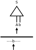
Assume we are using predictive parsing and, as illustrated in the diagram to the right, we are at A in the parse tree and b in the input. Since lookahead=b and b is in FIRST(RHS) for the bottom A production, we would choose that production to expand A. But this could be wrong! Remember that we don't look ahead in the tree just in the input. So we would not have noticed that the next node in the tree (i.e., in the frontier) is b. This is possible since b is in FOLLOW(A). So perhaps we should use the second A production to produce ε in the tree, and then the next node b would match the input b.
The goal is to produce a table telling us at each situation which
production to apply.
A situation
means a nonterminal in the parse tree and an
input symbol in lookahead.
So we produce a table with rows corresponding to nonterminals and columns corresponding to input symbols (including $, the endmarker). In an entry we put the production to apply when we are in that situation.
We start with an empty table M and populate it as follows. (2e has typo; it has FIRST(A) instead of FIRST(α).) For each production A → α
strange) condition above. If ε is in FIRST(α), then α⇒*ε. Hence we could (should??) apply the production A→α, have the α go to ε and then the b (or $), which follows A will match the b in the input.
When we have finished filling in the table M, what do we do if an slot has
LL(1) grammarsSomeone erred when they said the grammar generated an LL(1) language. Since the language is not LL(1), we must use a different technique. One possibility is to use bottom-up parsing, which we study next. Another is to modify the procedure for this non-terminal to look further ahead (typically one more token) to decide what action to perform.
Example: Work out the parsing table for
    E  → T E'
    E' → + T E' | ε
    T  → F T'
    T' → * F T' | ε
    F  → ( E ) | id
| FIRST | FOLLOW | |
|---|---|---|
| E | ( id | $ ) |
| E' | ε + | $ ) |
| T | ( id | + $ ) |
| T' | ε * | + $ ) |
| F | ( id | * + $ ) |
We already computed FIRST and FOLLOW as shown on the right. The table skeleton is
| Nonter- minal | Input Symbol | |||||
|---|---|---|---|---|---|---|
| + | * | ( | ) | id | $ | |
| E | ||||||
| E' | ||||||
| T | ||||||
| T' | ||||||
| F | ||||||
Homework: Produce the predictive parsing table for
This illustrates the standard technique for eliminating recursion by keeping the stack explicitly. The runtime improvement can be considerable.
Skipped.
Now we start with the input string, i.e., the bottom (leaves) of what will become the parse tree, and work our way up to the start symbol.
For bottom up parsing, we are not as fearful of left recursion as we were with top down. Our first few examples will use the left recursive expression grammar
    E → E + T | T
    T → T * F | F
    F → ( E ) | id
Remember that running a production in reverse
, i.e., replacing
the RHS by the LHS is called reducing.
So our goal is to reduce the input string to the start symbol.
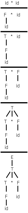
On the right is a movie of parsing id*id in a bottom-up fashion. Note the way it is written. For example, from step 1 to 2, we don't just put F above id*id. We draw it as we do because it is the current top of the tree (really forest) and not the bottom that we are working on so we want the top to be in horizontal line and hence easy to read.
The tops of the forest are the roots of the subtrees present in the
diagram.
For the movie those are
id * id, F * id, T * F, T, E
Note that (since the reduction successfully reaches the start
symbol) each of these sets of roots is a sentential form.
The steps from one frame of the movie, when viewed going down the
page, are reductions (replace the RHS of a production by the LHS).
Naturally, when viewed going up the page, we have a derivation
(replace LHS by RHS).
For our example the derivation is
E ⇒ T ⇒ T * F ⇒
T * id ⇒ F * id ⇒ id * id
Note that this is a rightmost derivation and hence each of the sets of roots identified above is a right sentential form. So the reduction we did in the movie was a rightmost derivation in reverse.
Remember that for a non-ambiguous grammar there is only one rightmost derivation and hence there is only one rightmost derivation in reverse.
Remark: You cannot simply scan the string (the
roots of the forest) from left to right and choose the first
substring that matches the RHS of some production.
If you try it in our movie you will reduce T to E right after T
appears.
The result is not a right sentential form.
| Right Sentential Form | Handle | Reducing Production |
|---|---|---|
| id1 * id2 | id1 | F → id |
| F * id2 | F | T → F |
| T * id2 | id2 | F → id |
| T * F | T * F | E → T * F |
The strings that are reduced during the reverse of a rightmost derivation are called the handles. For our example, this is shown in the table on the right.
Note that the string to the right of the handle must contain only terminals. If there was a non-terminal to the right, it would have been reduced in the RIGHTmost derivation that leads to this right sentential form.
Often instead of referring to a derivation A→α as a handle, we call α the handle. I should say a handle because there can be more than one if the grammar is ambiguous.
So (assuming a non-ambiguous grammar) the rightmost derivation in reverse can be obtained by constantly reducing the handle in the current string.
Homework: 4.23 a c
We use two data structures for these parsers.
shifted(see below) onto the stack will be terminals, but some are
reducedto nonterminals. The bottom of the stack is marked with $ and initially the stack is empty (i.e., has just $).
| Stack | Input | Action |
|---|---|---|
| $ | id1*id2$ | shift |
| $id1 | *id2$ | reduce F→id |
| $F | *id2$ | reduce T→F |
| $T | *id2$ | shift |
| $T* | id2$ | shift |
| $T*id2 | $ | reduce F→id |
| $T*F | $ | reduce T→T*F |
| $T | $ | reduce E→T |
| $E | $ | accept |
A technical point, which explains the usage of a stack is that a handle is always at the TOS. See the book for a proof; the idea is to look at what rightmost derivations can do (specifically two consecutive productions) and then trace back what the parser will do since it does the reverse operations (reductions) in the reverse order.
We have not yet discussed how to decide whether to shift or reduce when both are possible. We have also not discussed which reduction to choose if multiple reductions are possible. These are crucial question for bottom up (shift-reduce) parsing and will be addressed.
Homework: 4.23 b
There are grammars (non-LR) for which no viable algorithm can decide whether to shift or reduce when both are possible or which reduction to perform when several are possible. However, for most languages, choosing a good lexer yields an LR(k) language of tokens. For example, ada uses () for both function calls and array references. If the lexer returned id for both array names and procedure names then a reduce/reduce conflict would occur when the stack was ... id ( id and the input ) ... since the id on TOS should be reduced to parameter if the first id was a procedure name and to expr if the first id was an array name. A better lexer (and an assumption, which is true in ada, that the declaration must precede the use) would return proc-id when it encounters a lexeme corresponding to a procedure name. It does this by constructing the symbol table it builds.
I will have much more to say about SLR than the other LR schemes. The reason is that SLR is simpler to understand, but does capture the essence of shift-reduce, bottom-up parsing. The disadvantage of SLR is that there are LR grammars that are not SLR.
The text's presentation is somewhat controversial.
Most commercial compilers use hand-written top-down parsers of the
recursive-descent (LL not LR) variety.
Since the grammars for these languages are not LL(1), the
straightforward application of the techniques we have seen will not
work.
Instead the parsers actually look ahead further than one token, but
only at those few places where the grammar is in fact not LL(1).
Recall that (hand written) recursive descent compilers have a
procedure for each nonterminal so we can customize as needed
.
These compiler writers claim that they are able to produce much
better error messages than can readily be obtained by going to LR
(with its attendant requirement that a parser-generator be used since
the parsers are too large to construct by hand).
Note that compiler error messages is a very important user interface
issue and that with recursive descent one can augment the procedure
for a nonterminal with statements like
if (nextToken == X) then error(expected Y here
)
Nonetheless, the claims made by the text are correct, namely.
We now come to grips with the big question
:
How does a shift-reduce parser know when to shift and when to
reduce?
This will take a while to answer in a satisfactory manner.
The unsatisfactory answer is that the parser has tables that say in
each situation
whether to shift or reduce (or announce error,
or announce acceptance).
To begin the path toward the answer, we need several definitions.
An item is a production with a marker saying how far the parser has gotten with this production. Formally,
Definition: An (LR(0)) item of a grammar is a production with a dot added somewhere to the RHS.
Examples:
The item E → E · + T signifies that the parser has just processed input that is derivable from E and will look for input derivable from + T.
Line 4 indicates that the parser has just seen the entire
RHS and must consider reducing it to E.
Important: consider reducing
does not mean
reduce
.
The parser groups certain items together into states. As we shall see, the items with a given state are treated similarly.
Our goal is to construct first the canonical LR(0)
collection of states and then a DFA called the LR(0) automaton
(technically not a DFA since it has no dead state
).
To construct the canonical LR(0) collection formally and present the parsing algorithm in detail we shall
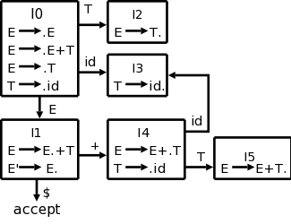
Augmenting the grammar is easy. We simply add a new start state S' and one production S'→S· The purpose is to detect success, which occurs when the parser is ready to reduce S to S'.
So our example grammar
    E → E + T | T
    T → T * F | F
    F → ( E ) | id
is augmented by adding the production E' → E·.
I hope the following interlude will prove helpful. In preparing to present SLR, I was struck how it looked like we were working with a DFA that came from some (unspecified and unmentioned) NFA. It seemed that by first doing the NFA, I could give some rough insight. Since for our current example the NFA has more states and hence a bigger diagram, let's consider the following extremely simple grammar.
    E → E + T
    E → T
    T → id
When augmented this becomes
   E' → E
    E → E + T
    E → T
    T → id
When the dots are added we get 10 items (4 from the second
production, 2 each from the other three).
See the diagram at the right.
We begin at E'→.E since it is the start item.
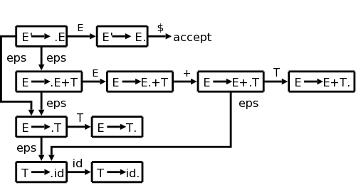
Note that there are really four kinds
of edges.
If we were at the item E→E·+T (the dot indicating that we have seen an E and now need a +) and shifted a + from the input to the stack we would move to the item E→E+·T. If the dot is before a non-terminal, the parser needs a reduction with that non-terminal as the LHS.
Now we come to the idea of closure, which I illustrate in the diagram with the ε's. Please note that this is rough, we are not doing regular expressions again, but I hope this will help you understand the idea of closure, which like ε in regular production leads to nondeterminism.
Look at the start state. The placement of the dot indicates that we next need to see an E. Since E is a nonterminal, we won't see it in the input, but will instead have to generate it via a production. Thus by looking for an E, we are also looking for any production that has E on the LHS. This is indicated by the two ε's leaving the top left box. Similarly, there are ε's leaving the other three boxes where the dot is immediately to the left of a nonterminal.
 As with regular expressions, we combine
 n-items
connected by
an ε arc into a d-item
.
The actual terminology used is that we combine these items into a
set of items (later referred to as a state).
There is another combination that occurs.
The top two n-items in the left column are combined into the same
d-item and both n-items have E transitions (outgoing arcs labeled
E).
Since we are considering these two n-items to be the same d-item and
the arcs correspond to the same transition, the two targets (the
top two n-items in the 2nd column) are combined.
A d-item has all the outgoing arcs of the original n-items
it contains.
This is the way we converted an NFAs into a DFA in the previous
chapter.