================ Start Lecture #5 ================
Remark: Please don't confuse the homework numbers. An assignment like 6 if given in section 5.2.4 means that you go to the problems section of 5.2 (which is 5.2.x for x the largest possible value) and do problem 6 there. The problem would be labeled 5.2.6.
How lexer-generators like Lex work. Since your lab2 is to produce a lexer, this is also a section on how you should solve lab2.
We have seen simulators for DFAs and NFAs.
The remaining large question is how is the lex input converted into one of these automatons.
Also
In this section we will use transition graphs. Of course lexer-generators do not draw pictures; instead they use the equivalent transition tables.
Recall that the regular definitions in Lex are mere conveniences
that can easily be converted to REs and hence we need only convert
REs into an FSA.
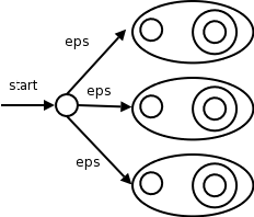
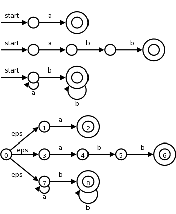
We already know how to convert a single RE into an NFA. But lex input will contain several REs (since it wishes to recognize several different tokens). The solution is to
Label each of the accepting states (for all NFAs constructed in step 1) with the actions specified in the lex program for the corresponding pattern.
We use the algorithm for simulating NFAs presented in 3.7.2.
The simulator starts reading characters and calculates the set of states it is at.
At some point the input character does not lead to any state or we have reached the eof. Since we wish to find the longest lexeme matching the pattern we proceed backwards from the current point (where there was no state) until we reach an accepting state (i.e., the set of NFA states, N-states, contains an accepting N-state). Each accepting N-state corresponds to a matched pattern. The lex rule is that if a lexeme matches multiple patterns we choose the pattern listed first in the lex-program.
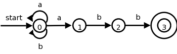
| Pattern | Action to perform |
|---|---|
| a | Action1 |
| abb | Action2 |
| a*bb* | Action3 |
Consider the example on the right with three patterns and their
associated actions and consider processing the input aaba.
optimization.
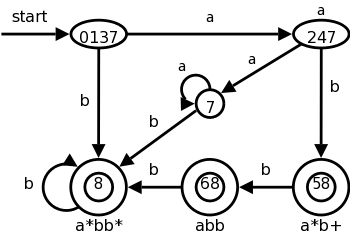
We could also convert the NFA to a DFA and simulate that. The resulting DFA is on the right. Note that it shows the same D-states (i.e., sets of N-states) we saw in the previous section, plus some other D-states that arise from inputs other than aaba.
We label the accepting states with the pattern matched. If multiple patterns are matched (because the accepting D-state contains multiple accepting N-states), we use the first pattern listed (assuming we are using lex conventions).
Technical point. For a DFA, there must be a outgoing edge from each D-state for each possible character. In the diagram, when there is no NFA state possible, we do not show the edge. Technically we should show these edges, all of which lead to the same D-state, called the dead state, and corresponds to the empty subset of N-states.
There are trade-offs depending on how much you want to do by hand and how much you want to program. At the extreme you could write a program that reads in the regular expression for the tokens and produces a lexer, i.e., you could write a lexical-analyzer-generator. I very much advise against this, especially since the first part of the lab requires you to draw the transition diagram anyway.
The two reasonable alternatives are.
This has some tricky points; we are basically skipping it. This lookahead operator is for when you must look further down the input but the extra characters matched are not part of the lexeme. We write the pattern r1/r2. In the NFA we match r1 then treat the / as an ε and then match s1. It would be fairly easy to describe the situation when the NFA has only one ε-transition at the state where r1 is matched. But it is tricky when there are more than one such transition.
Skipped
Skipped
Skipped
Skipped
Skipped
Homework: Read Chapter 4.
As we saw in the previous chapter the parser calls the lexer to obtain the next token.
Conceptually, the parser accepts a sequence of tokens and produces a parse tree. In practice this might not occur.
There are three classes for grammar-based parsers.
The universal parsers are not used in practice as they are inefficient; we will not discuss them.
As expected, top-down parsers start from the root of the tree and proceed downward; whereas, bottom-up parsers start from the leaves and proceed upward.
The commonly used top-down and bottom parsers are not universal. That is, there are (context-free) grammars that cannot be used with them.
The LL and LR parsers are important in practice. Hand written parsers are often LL. Specifically, the predictive parsers we looked at in chapter two are for LL grammars.
The LR grammars form a larger class. Parsers for this class are usually constructed with the aid of automatic tools.
Expressions with + and *
    E → E + T | T
    T → T * F | F
    F → ( E ) | id
This takes care of precedence, but as we saw before, gives us trouble since it is left-recursive and we did top-down parsing. So we use the following non-left-recursive grammar that generates the same language.
    E  → T E'
    E' → + T E' | ε
    T  → F T'
    T' → * F T' | ε
    F  → ( E ) | id
The following ambiguous grammar will be used for illustration, but in general we try to avoid ambiguity. This grammar does not enforce precedence.
E → E + E | E * E | ( E ) | id
There are different levels
of errors.
off by oneusage of < instead of <=.
The goals are clear, but difficult.
Print an error message when parsing cannot continue and then terminate parsing.
The first level improvement. The parser discards input until it encounters a synchronizing token. These tokens are chosen so that the parser can make a fresh beginning. Good examples are ; and }.
Locally replace some prefix of the remaining input by some string. Simple cases are exchanging ; with , and = with ==. Difficulties occur when the real error occurred long before an error was detected.
Include productions for common errors
.
Change the input I to the closest
correct input I' and
produce the parse tree for I'.
I don't use these without saying so.
This is mostly (very useful) notation.
Assume we have a production A → α.
We would then say that A derives α and write
A ⇒ α
We generalize this.
If, in addition, β and γ are strings, we say that
βAγ derives βαγ and write
βAγ ⇒ βαγ
We generalize further.
If x derives y and y derives z, we say x derives z and write
x ⇒* z.
The notation used is ⇒ with a * over it (I don't see it in
html).
This should be read derives in zero or more steps
.
Formally,
Definition: If S is the start symbol and S ⇒* x, we say x is a sentential form of the grammar.
A sentential form may contain nonterminals and terminals. If it contains only terminals it is a sentence of the grammar and the language generated by a grammar G, written L(G), is the set of sentences.
Definition: A language generated by a (context-free) grammar is called a context free language.
Definition: Two grammars generating the same language are called equivalent.
Examples: Recall the ambiguous grammar above
E → E + E | E * E | ( E ) | id
We see that id + id is a sentence.
Indeed it can be derived in two ways from the start symbol E.
    E ⇒ E + E ⇒ id + E ⇒ id + id
    E ⇒ E + E ⇒ E + id ⇒ id + id
In the first derivation, we replaced the leftmost nonterminal by the body of a production having the nonterminal as head. This is called a leftmost derivation. Similarly the second derivation in which the rightmost nonterminal is replaced is called a rightmost derivation or a canonical derivation.
When one wishes to emphasize that a (one step) derivation is leftmost they write an lm under the ⇒. To emphasize that a (general) derivation is leftmost, one writes an lm under the ⇒*. Similarly one writes rm to indicate that a derivation is rightmost. I won't do this in the notes but will on the board.
Definition: If x can be derived using a leftmost derivation, we call x a left-sentential form. Similarly for right-sentential form.
Homework: 1(ab), 2(ab).
The leaves of a parse tree (or of any other tree), when read left to right, are called the frontier of the tree. For a parse tree we also call them the yield of the tree.
If you are given a derivation starting with a single nonterminal,
A ⇒ x1 ⇒ x2 ... ⇒ xn
it is easy to write a parse tree with A as the root and
xn as the leaves.
Just do what (the production contained in) each step of the
derivation says.
The LHS of each production is a nonterminal in the frontier of the
current tree so replace it with the RHS to get the next tree.
Do this for both the leftmost and rightmost derivations of id+id above.
So there can be many derivations that wind up with the same final tree.
But for any parse tree there is a unique leftmost derivation the
produces that tree (always choose the leftmost unmarked nonterminal
to be the LHS and mark it).
Similarly, there is a unique rightmost derivation that produces the
tree.
There may be others as well (e.g., sometime choose the leftmost
unmarked nonterminal to expand and other times choose the rightmost;
or choose a
middle
unmarked nonterminal).
Homework: 1c
Recall that an ambiguous grammar is one for which there is more than one parse tree for a single sentence. Since each parse tree corresponds to exactly one leftmost derivation, a grammar is ambiguous if and only if it permits more than one leftmost derivation of a given sentence. Similarly, a grammar is ambiguous if and only if it permits more than one rightmost of a given sentence.
We know that the grammar
E → E + E | E * E | ( E ) | id
is ambiguous because we have seen (a few lectures ago) two parse
trees for
    E ⇒ E + E          E ⇒ E * E
      ⇒ id + E           ⇒ E + E * E
      ⇒ id + E * E       ⇒ id + E * E
      ⇒ id + id * E      ⇒ id + id * E
      ⇒ id + id * id     ⇒ id + id * E
As we stated before we prefer unambiguous grammars. Failing that, we want disambiguation rules.
Skipped
Alternatively context-free languages vs regular languages.
Given an RE, construct an NFA as in chapter 3.
From that NFA construct a grammar as follows.
If you trace an NFA accepting a sentence, it just corresponds to the constructed grammar deriving the same sentence. Similarly, follow a derivation and notice that at any point prior to acceptance there is only one nonterminal; this nonterminal gives the state in the NFA corresponding to this point in the derivation.
The book starts with (a|b)*abb and then uses the short NFA on the left below. Recall that the NFA generated by our construction is the longer one on the right.
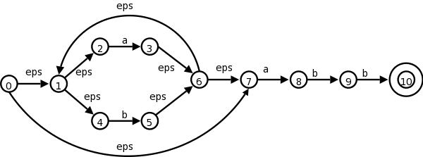
The book gives the simple grammar for the short diagram.
Let's be ambitious and try the long diagram
    A0 → A1 | A7
    A1 → A2 | A4
    A2 → a A3
    A3 → A6
    A4 → b A5
    A5 → A6
    A6 → A1 | A7
    A7 → a A8
    A8 → b A9
    A9 → b A10
    A10 → ε
Now trace a path in the NFA and see that it is just a derivation. The same is true in reverse (derivation gives path). The key is that at every stage you have only one nonterminal.
The grammar
A → a A b | ε
generates all strings of the form anbn, where
there are the same number of a's and b's.
In a sense the grammar has counted.
No RE can generate this language (proof in book).
Why have separate lexer and parser?
Recall the ambiguous grammar with the notorious dangling
else
problem.
    stmt → if expr then stmt
         | if expr then stmt else stmt
         | other
This has two leftmost derivations for
if E1 then S1 else if E2 then S2 else S3
Do these on the board. They differ in the beginning.
In this case we can find a non-ambiguous, equivalent grammar.
        stmt → matched-stmt | open-stmt
matched-stmp → if expr then matched-stmt else matched-stmt
	     | other
   open-stmt → if expr then stmt
	     | if expr then matched-stmt else open-stmt
On the board try to find leftmost derivations of the problem sentence above.
We did special cases in chapter 2.
Now we do it right
(tm).
Previously we did it separately for one production and for two productions with the same nonterminal on the LHS. Not surprisingly, this can be done for n such productions (together with other non-left recursive productions involving the same nonterminal).
Specifically we start with
A → A x1 | A x2 | ... A xn | y1 | y2 | ... ym
where the x's and y's are strings, no x is ε, and no y
begins with A.
The equivalent non-left recursive grammar is
    A  → y1 A' | ... | ym A'
    A' → x1 A' | ... | xn A' | ε
The idea is as follows. Look at the left recursive grammar. At some point you stop producing more As and have the A (which is on the left) become one of the ys. So the final string starts with a y. Up to this point all the As became xA for one of the xs. So the final string is a y followed by a bunch of xs, which is exactly what the non-left recursive definition says.
Example: Assume n=m=1, x1 is + and y1 is *.
With the recursive grammar, we have the following lm derivation.
A ⇒ A + ⇒ A + + ⇒ * + +
With the non-recursive grammar we have
A ⇒ * A' ⇒ * + A' ⇒ * + + A' ⇒ * + +
This removes direct left recursion where a production with A on the left hand side begins with A on the right. If you also had direct left recursion with B, you would apply the procedure twice.
The harder general case is where you permit indirect left recursion, where, for example one production has A as the LHS and begins with B on the RHS, and a second production has B on the LHS and begins with A on the RHS. Thus in two steps we can turn A into something starting again with A. Naturally, this indirection can involve more than 2 nonterminals.
Theorem: All left recursion can be eliminated.
Proof: The book proves this for grammars that have
no ε-productions and no cycles
and has exercises
asking the reader to prove that cycles and ε-productions can
be eliminated.
We will try to avoid these hard cases.
Homework: Eliminate left recursion in the
following grammar for simple postfix expressions.
S → S S + | S S * | a
If two productions with the same LHS have their RHS beginning with the same symbol, then the FIRST sets will not be disjoint so predictive parsing (chapter 2) will be impossible and more generally top down parsing (defined later this chapter) will be more difficult as a longer lookahead will be needed to decide which production to use.
So convert A → x y1 | x y2 into
    A → x A'
   A' → y1 | y2
In other words factor outthe x.
Homework: Left factor your answer to the previous homework.
Although our grammars are powerful, they are not all-powerful. For example, we cannot write a grammar that checks that all variables are declared before used.
We did an example of top down parsing, namely predictive parsing, in chapter 2.
For top down parsing, we
The above has two nondeterministic choices (the nonterminal, and the production) and requires luck at the end. Indeed, the procedure will generate the entire language. So we have to be really lucky to get the input string.
Let's reduce the nondeterminism in the above algorithm by specifying which nonterminal to expand. Specifically, we do a depth-first (left to right) expansion. This corresponds to a leftmost derivation.
We leave the choice of production nondeterministic.
We also process the terminals in the RHS, checking that they match the input. By doing the expansion depth-first, left to right, we ensure that we encounter the terminals in the order they will appear in the frontier of the final tree. Thus if the terminal does not match the corresponding input symbol now, it never will and the expansion so far will not produce the input string as desired.
Now our algorithm is
for i = 1 to n
  if Xi is a nonterminal
    process Xi  // recursive
  else if Xi (a terminal) matches current input symbol
    advance input to next symbol
  else // trouble Xi doesn't match and never will
Note that the trouble
mentioned at the end of the algorithm
does not signify an erroneous input.
We may simply have chosen the wrong
production in step 2.
In a general recursive descent (top-down) parser, we would support backtracking, that is when we hit the trouble, we would go back and choose another production. Since this is recursive, it is possible that no productions work for this nonterminal, because the wrong choice was made earlier.
The good news is that we will work with grammars where we can control the nondeterminism much better. Recall that for predictive parsing, the use of 1 symbol of lookahead made the algorithm fully deterministic, without backtracking.
We used FIRST(RHS) when we did predictive parsing.
Now we learn the whole truth about these two sets, which proves to be quite useful for several parsing techniques (and for error recovery).
The basic idea is that FIRST(α) tells you what the first symbol can be when you fully expand the string α and FOLLOW(A) tells what terminals can immediately follow the nonterminal A.
Definition: For any string α of grammar symbols, we define FIRST(α) to be the set of terminals that occur as the first symbol in a string derived from α. So, if α⇒*xQ for x a terminal and Q a string, then x is in FIRST(α). In addition if α⇒*ε, then ε is in FIRST(α).
Definition: For any nonterminal A, FOLLOW(A) is the set of terminals x, that can appear immediately to the right of A in a sentential form. Formally, it is the set of terminals x, such that S⇒*αAxβ. In addition, if A can be the rightmost symbol in a sentential form, the endmarker $ is in FOLLOW(A).
Note that there might have been symbols between A and x during the derivation, providing they all derived ε and eventually x immediately follows A.
Unfortunately, the algorithms for computing FIRST and FOLLOW are not as simple to state as the definition suggests, in large part caused by ε-productions.