Compilers
================ Start Lecture #1 ================
G22.2130: Compiler Construction
2006-07 Spring
Allan Gottlieb
Tuesday 5-6:50pm Rm 109 Ciww
Chapter 0: Administrivia
I start at Chapter 0 so that when we get to chapter 1, the
numbering will agree with the text.
0.1: Contact Information
- <my-last-name> AT nyu DOT edu (best method)
- http://cs.nyu.edu/~gottlieb
- 715 Broadway, Room 712
- 212 998 3344
0.2: Course Web Page
There is a web site for the course.
You can find it from my home page listed above.
- You can also find these lecture notes on the course home page.
Please let me know if you can't find it.
- The notes are updated as bugs are found or improvements made.
- I will also produce a separate page for each lecture after the
lecture is given.
These individual pages might not get updated as quickly as the
large page.
0.3: Textbook
The course text is Aho, Lam, Seithi, and Ullman:
Compilers: Principles, Techniques, and Tools,
second edition
- Available in bookstore.
- We will cover most of the first 8 chapters (plus some asides).
- The first edition is a descendant of the classic
Principles of Compiler Design
- Independent of the titles, each of the books is called
“The Dragon Book”, due to the cover picture.
0.4: Computer Accounts and Mailman Mailing List
- You are entitled to a computer account on one of the departmental
sun machines.
If you do not have one already, please get it asap.
- Sign up for the Mailman mailing list for the course.
You can do so by clicking
here
- If you want to send mail just to me, use the address given above, not
the mailing list.
- Questions on the labs should go to the mailing list.
You may answer questions posed on the list as well.
Note that replies are sent to the list.
- I will respond to all questions; if another student has answered the
question before I get to it, I will confirm if the answer given is
correct.
- Please use proper mailing list etiquette.
- Send plain text messages rather than (or at least in
addition to) html.
- Use Reply to contribute to the current thread, but NOT
to start another topic.
- If quoting a previous message, trim off irrelevant parts.
- Use a descriptive Subject: field when starting a new topic.
- Do not use one message to ask two unrelated questions.
- Do NOT make the mistake of sending your completed lab
assignment to the mailing list.
This is not a joke; several students have made this mistake in
past semesters.
0.5: Grades
Your grade will be a function of your final exam and laboratory
assignments (see below).
I am not yet sure of the exact weightings
for each lab and the final, but the final will be roughly half the
grade (very likely between 40% and 60%).
0.6: The Upper Left Board
I use the upper left board for lab/homework assignments and
announcements.
I should never erase that board.
If you see me start to erase an announcement, please let me know.
I try very hard to remember to write all announcements on the upper
left board and I am normally successful.
If, during class, you see
that I have forgotten to record something, please let me know.
HOWEVER, if I forgot and no one reminds me, the
assignment has still been given.
0.7: Homeworks and Labs
I make a distinction between homeworks and labs.
Labs are
- Required.
- Due several lectures later (date given on assignment).
- Graded and form part of your final grade.
- Penalized for lateness.
- Most often are computer programs you must write.
Homeworks are
- Optional.
- Due the beginning of Next lecture.
- Not accepted late.
- Mostly from the book.
- Collected and returned.
- Able to help, but not hurt, your grade.
0.7.1: Homework Numbering
Homeworks are numbered by the class in which they are assigned. So
any homework given today is homework #1. Even if I do not give
homework today, the homework assigned next class will be homework
#2. Unless I explicitly state otherwise, all homeworks assignments
can be found in the class notes. So the homework present in the
notes for lecture #n is homework #n (even if I inadvertently forgot
to write it to the upper left board).
0.7.2: Doing Labs on non-NYU Systems
You may solve lab assignments on any system you wish, but ...
- You are responsible for any non-nyu machine.
I extend deadlines if the nyu machines are down, not if yours are.
- Be sure to upload your assignments to the
nyu systems.
- In an ideal world, a program written in a high level language
like Java, C, or C++ that works on your system would also work
on the NYU system used by the grader.
Sadly this ideal is not always achieved despite marketing
claims to the contrary.
So, although you may develop you lab on any system,
you must ensure that it runs on the nyu system assigned to the
course.
- If somehow your assignment is misplaced by me and/or a grader,
we need a to have a copy ON AN NYU SYSTEM
that can be used to verify the date the lab was completed.
- When you complete a lab (and have it on an nyu system), do
not edit those files. Indeed, put the lab in a separate
directory and keep out of the directory. You do not want to
alter the dates.
0.7.3: Obtaining Help with the Labs
Good methods for obtaining help include
- Asking me during office hours (see web page for my hours).
- Asking the mailing list.
- Asking another student, but ...
Your lab must be your own.
That is, each student must submit a unique lab.
Naturally, simply changing comments, variable names, etc. does
not produce a unique lab.
0.7.4: Computer Language Used for Labs
You may write your lab in Java, C, or C++.
Other languages may be possible, but please ask in advance.
I need to ensure that the TA is comfortable with the language.
0.8: A Grade of “Incomplete”
The rules for incompletes and grade changes are set by the school
and not the department or individual faculty member.
The rules set by GSAS state:
The assignment of the grade Incomplete Pass(IP)
or Incomplete Fail(IF) is at the discretion of
the instructor. If an incomplete grade is not
changed to a permanent grade by the instructor
within one year of the beginning of the course,
Incomplete Pass(IP) lapses to No Credit(N), and
Incomplete Fail(IF) lapses to Failure(F).
Permanent grades may not be changed unless the
original grade resulted from a clerical error.
0.9: An Introductory Compiler Course with a Programming Prerequisite
0.9.1: This is an introductory course ...
I do not assume you have had a compiler course as an undergraduate,
and I do not assume you have had experience
developing/maintaining a compiler.
If you have already had a compiler class,
this course is probably not appropriate.
For example, if you can explain the following concepts/terms,
the course is probably too elementary for you.
- Parsing
- Lexical Analysis
- Syntax analysis
- Register allocation
- LALR Grammar
... with a Programming Prerequisite
I do assume you are an experienced programmer.
There will be
non-trivial programming assignments during this course.
Indeed, you
will write a compiler for a simple programming language.
I also assume that you have at least a passing familiarity with
assembler language.
In particular, your compiler may need to produce
assembler language.
We will also be using addressing modes found in typical assemblers.
We will not, however, write significant
assembly-language programs.
0.10: Academic Integrity Policy
Our policy on academic integrity, which applies to all graduate
courses in the department, can be found
here.
Roadmap of the Course
- Chapter 1 touches on all the material.
- Chapter 2 constructs (the front end of) a simple compiler.
- Chapters 3-8 fill in the (considerable) gaps, as well as
the beginnings of the back end.
- I tend to spend too much time on introductory chapters, but will
try not to.
Chapter 1: Introduction to Compiling
Homework Read chapter 1.
1.1: Language Processors
A Compiler is a translator from one language, the input
or source language, to another language, the output
or target language.
Often, but not always, the target language is an assembler language
or the machine language for a computer processor.
Note that using a compiler requires a two step process to run a
program.
- Execute the compiler (and possibly an assembler) to translate
the source program into a machine language program.
- Execute the resulting machine language program, supplying
appropriate input.
This should be compared with an interpreter, which accepts
the source language program and the appropriate
input, and itself produces the program output.
Sometimes both compilation and interpretation are used.
For example, consider typical Java implementations.
The (Java) source code is translated (i.e., compiled)
into bytecodes, the machine language for an
idealized virtual machine
, the Java Virtual Machine or JVM.
Then an interpreter of the JVM (itself normally called a JVM)
accepts the bytecodes and the appropriate input,
and produces the output.
This technique was quite popular in academia, with the Pascal
programming language and P-code.
The compilation tool chain
For large programs, the compiler is actually part of a multistep
tool chain
[preprocessor] → [compiler] → [assembler]
→ [linker] → [loader]
We will be primarily focused on the second element of the chain,
the compiler.
Our target language will be assembly language.
I give a very short description of the other components, including
some historical comments.
Preprocessors
Preprocessors are normally fairly simple as in the C language,
providing primarily the ability to include files and expand macros.
There are exceptions, however.
IBM's PL/I, another Algol-like language had quite an extensive
preprocessor, which made available at preprocessor time, much of the
PL/I language itself (e.g., loops and I believe procedure calls).
Some preprocessors essentially augment the base language, to add
additional capabilities.
One could consider them as compilers in their own right, having as
source this augmented language (say Fortran augmented with
statements for multiprocessor execution in the guise of Fortran
comments) and as target the original base language (in this case
Fortran).
Often the “preprocessor” inserts procedure calls to
implement the extensions at runtime.
Assemblers
Assembly code is an mnemonic version of machine code in which
names, rather than binary values, are used for machine instructions,
and memory addresses.
Some processors have fairly regular operations and as a result
assembly code for them can be fairly natural and not-too-hard to
understand.
Other processors, in particular Intel's x86 line, have let us
charitably say more interesting
instructions with certain
registers used for certain things.
My laptop has one of these latter processors (pentium 4) so my gcc
compiler produces code that from a pedagogical viewpoint is less
than ideal.
If you have a mac with a ppc processor (newest macs are x86), your
assembly language is cleaner.
NYU's ACF features sun computers with sparc processors, which also
have regular instruction sets.
Two pass assembly
No matter what the assembly language is, an assembler needs to
assign memory locations to symbols (called identifiers) and use the
numeric location address in the target machine language produced.
Of course the same address must be used for all occurrences of a
given identifier and two different identifiers must (normally) be
assigned two different locations.
The conceptually simplest way to accomplish this is to make two
passes over the input (read it once, then read it again from the
beginning).
During the first pass, each time a new identifier is
encountered, an address is assigned and the pair (identifier,
address) is stored in a symbol table.
During the second
pass, whenever an identifier is encountered, its address is looked
up in the symbol table and this value is used in the generated
machine instruction.
Linkers
Linkers, a.k.a. linkage editors combine the output of the assembler
for several different compilations.
That is the horizontal line of
the diagram above should really be a collection of lines converging
on the linker.
The linker has another input, namely libraries, but
to the linker the libraries look like other programs compiled and
assembled.
The two primary tasks of the linker are
- Relocating relative addresses.
- Resolving external references (such as the procedure xor() above).
Relocating relative addresses
The assembler processes one file at a time.
Thus the symbol table
produced while processing file A is independent of the symbols
defined in file B, and conversely.
Thus, it is likely that the same
address will be used for different symbols in each program.
The
technical term is that the (local) addresses in the symbol table for
file A are relative to file A; they must be relocated
by the linker.
This is accomplished by adding the starting address
of file A (which in turn is the sum of the lengths of all the files
processed previously in this run) to the relative address.
Resolving external references
Assume procedure f, in file A, and procedure g, in file B, are
compiled (and assembled) separately.
Assume also that f invokes g.
Since the compiler and assembler do not see g when processing f, it
appears impossible for procedure f to know where in memory to find
g.
The solution is for the compiler to indicated in the output of the
file A compilation that the address of g is needed.
This is called a use of g.
When processing file B, the compiler outputs the (relative) address
of g.
This is called the definition of g.
The assembler passes this information to the linker.
The simplest linker technique is to again make two passes.
During the first pass, the linker records in its “external
symbol table” (a table of external symbols, not a symbol table
that is stored externally) all the definitions encountered.
During the second pass, every use can be resolved by access to the
table.
I will be covering the linker in more detail tomorrow at 5pm in
2250, OS Design
Loaders
After the linker has done its work, the resulting “executable
file” can be loaded by the operating system into central
memory.
The details are OS dependent.
With early single-user
operating systems all programs would be loaded into a fixed address
(say 0) and the loader simply copies the file to memory.
Today it
is much more complicated since (parts of) many programs reside in
memory at the same time.
Hence the compiler/assembler/linker cannot
know the real location for an identifier.
Indeed, this real location can change.
More information is given in any OS course
(e.g., 2250 given wednesdays at 5pm).
Homework: 1, 4
Remark
Unless state otherwise, homeworks are
from the book and specifically from the end of the second level
section we are discussing.
Even more specifically, we are in section 1.1, so you are to do the
first and fourth problem at the end of section 1.1.
These two problems are numbered 1.1.1 and 1.1.4 in the book.
End of Remark
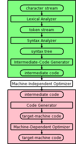
1.2: The Structure of a Compiler
Modern compilers contain two (large) parts, each of which is often
subdivided.
These two parts are the front end, shown in green on the right
and the back end, shown in pink.
The front end analyzes the source program, determines its
constituent parts, and constructs an intermediate representation of
the program.
Typically the front end is independent of the target language.
The back end synthesizes the target program from the
intermediate representation produced by the front end.
Typically the back end is independent of the source language.
This front/back division very much reduces the work for a compiling
system that can handle several (N) source languages and several (M)
target languages.
Instead of NM compilers, we need N front ends and M back ends.
For gcc (originally standing for Gnu C Compiler, but now standing
for Gnu Compiler Collection), N=7 and M~30 so the savings is
considerable.
Multiple Phases
The front and back end are themselves each divided into
multiple phases.
The input to each phase is the output of the previous.
Sometime a phase changes the representation of the input.
For example, the lexical analyzer converts a character stream input
into a token stream output.
Sometimes the representation is unchanged.
For example, the machine-dependent optimizer transforms
target-machine code into (hopefully improved) target-machine code.
The diagram is definitely not drawn to scale, in terms of effort or
lines of code.
In practice the optimizers, especially the machine-dependent one,
dominate.
Conceptually, there are three phases of analysis with the output of
one phase the input of the next.
The phases are called lexical analysis
or scanning, syntax analysis or parsing,
and semantic analysis.
1.2.1: Lexical Analysis (or Scanning)
The character stream input is grouped into meaningful units
called lexemes, which are then mapped
into tokens, the latter constituting the output of
the lexical analyzer.
For example, any one of the following
  x3 = y + 3;
  x3  =   y   +   3   ;
  x3   =y+ 3  ;
but not
x 3 = y + 3;
would be grouped into the lexemes x3, =, y, +, 3, and ;.
A token is a <token-name,attribute-value> pair.
For example
- The lexeme x3 would be mapped to a token such as <id,1>.
The name id is short for identifier.
The value 1 is the index of the entry for x3 in the symbol table
produced by the compiler.
This table is used to pass information to subsequent phases.
- The lexeme = would be mapped to the token <=>.
In reality it is probably mapped to a pair, whose second
component is ignored.
The point is that there are many different identifiers so we
need the second component, but there is only one assignment
symbol =.
- The lexeme y is mapped to the token <id,2>
- The lexeme + is mapped to the token <+>.
- The lexeme 3 is somewhat interesting and is discussed further
in subsequent chapters.
It is mapped to <number,something>, but what is the
something.
On the one hand there is only one 3 so we could just use the
token <number,3>.
However, there can be a difference between how this should be
printed (e.g., in an error message produced by subsequent
phases) and how it should be stored (fixed vs. float vs double).
Perhaps the token should point to the symbol table where an
entry for
this kind of 3
is stored.
Another possibility is to have a separate numbers table
.
- The lexeme ; is mapped to the token <;>.
Note that non-significant blanks are normally removed during
scanning.
In C, most blanks are non-significant.
Blanks inside strings are an exception.
Note that we can define identifiers, numbers, and the various
symbols and punctuation without using recursion (compare
with parsing below).
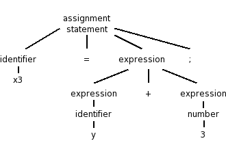
1.2.2: Syntax Analysis (or Parsing)
Parsing involves a further grouping in which tokens are grouped
into grammatical phrases, which are often represented in a parse
tree.
For example
x3 = y + 3;
would be parsed into the tree on the right.
This parsing would result from a grammar containing rules such as
    asst-stmt → id = expr ;
    expr      → number
              |  id
              |  expr + expr
Note the recursive definition of expression (expr). Note also the
hierarchical decomposition in the figure on the right.
The division between scanning and parsing is somewhat arbitrary,
but invariably if a recursive definition is involved, it is
considered parsing not scanning.
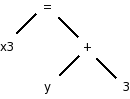
Often we utilize a simpler tree called the syntax tree with
operators as interior nodes and operands as the children of the
operator.
The syntax tree on the right corresponds to the parse
tree above it.
(Technical point.)
The syntax tree represents an assignment expression not an
assignment statement.
In C an assignment statement includes the trailing semicolon.
That is, in C (unlike in Algol) the semicolon is a statement
terminator not a statement separator.
1.2.3: Semantic Analysis
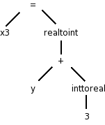
There is more to a front end than simply syntax.
The compiler
needs semantic information, e.g., the types (integer, real, pointer
to array of integers, etc) of the objects involved.
This enables
checking for semantic errors and inserting type conversion where necessary.
For example, if y was declared to be a real and x3 an integer, we
need to insert (unary, i.e., one operand) conversion operators
“inttoreal” and “realtoint” as shown on the
right.
1.2.4: Intermediate code generation
Many compilers first generate code for an “idealized
machine”.
For example, the intermediate code generated would assume that the
target has an unlimited number of registers and that any register
can be used for any operation.
Another common assumption is that machine operations take (up to) three
operands, two source and one target.
With these assumptions one generates three-address code
by
walking the semantic tree.
Our example C instruction would produce
temp1 = inttoreal(3)
temp2 = id2 + temp1
temp3 = realtoint(temp2)
id1 = temp3
We see that three-address code can include instructions
with fewer than 3 operands.
Sometimes three-address code is called quadruples because one can
view the previous code sequence as
inttoreal temp1 3     --
add       temp2 id2   temp1
realtoint temp3 temp2 --
assign    id1   temp3 --
Each “quad” has the form
operation target source1 source2
1.2.5: Code optimization
This is a very serious subject, one that we will not really
do justice to in this introductory course.
Some optimizations are fairly easy to see.
- Since 3 is a constant, the compiler can perform the int to
real conversion and replace the first two quads with
add temp2 id2 3.0
- The last two quads can be combined into
realtoint id1 temp2
1.2.6: Code generation
Modern processors have only a limited number of register.
Although some processors, such as the x86, can perform operations
directly on memory locations, we will for now assume only register
operations.
Some processors (e.g., the MIPS architecture) use three-address
instructions.
However, some processors permit only two addresses; the result
overwrites one of the sources.
With these assumptions, code something like the following would be
produced for our example, after first assigning memory locations to
id1 and id2.
    LD   R1,  id2
    ADDF R1,  R1, #3.0    // add float
    RTOI R2,  R1          // real to int
    ST   id1, R2
1.2.7: Symbol-Table Management
The the symbol table stores information about program variables
that will be used across phases.
Typically, this includes type information and storage location.
A possible point of confusion: the storage location
does not give the location where the compiler has
stored the variable.
Instead, it gives the location where the compiled program will store
the variable.
1.2.8: The Grouping of Phases into Passes
Logically each phase is viewed as a separate program that reads
input and produces output for the next phase, i.e., a pipeline.
In practice some phases are combined into a pass.
For example one could have the entire front end as one pass.
The term pass is used to indicate that the entire input is
read during this activity.
So two passes, means that the input is read twice.
We have discussed two pass approaches for both
assemblers
and linkers.
If we implement each phase separately and use multiple passes for
some of them, the compiler will perform a large number of I/O
operations, an expensive undertaking.
As a result techniques have been developed to reduce the number of
passes.
We will see in the next chapter how to combine the scanner, parser,
and semantic analyzer into one phase.
Consider the parser.
When it needs another token, rather than reading the input file
(presumably produced by the scanner), the parser calls the scanner
instead.
At selected points during the production of the syntax
tree, the parser calls the intermediate-code generator
which
performs semantic analysis as well as generating a portion of the
intermediate code.
For pedagogical reasons, we will not be employing this technique.
Thus your compiler will consist of separate programs for
the scanner, parser, and semantic analyzer / intermediate code
generator.
Indeed, these will very likely be labs 2, 3, and 4.
Reducing the number of passes
One problem with combining phases, or with implementing a single
phase in one pass, is that it appears that an internal form of the
entire program will need to be stored in memory.
This problem
arises because the downstream phase may need early in its execution,
information that the upstream phase produces only late in its
execution.
This motivates the use of symbol tables and a two pass approach.
However, a clever one-pass approach is often possible.
Consider the assembler (or linker).
The good case is when the definition precedes all uses so that the
symbol table contains the value of the symbol prior to that value
being needed.
Now consider the harder case of one or more uses preceding the
definition.
When a not-yet-defined symbol is first used, an entry is placed in
the symbol table, pointing to this use and indicating that the
definition has not yet appeared.
Further uses of the same symbol attach their addresses to a linked
list of “undefined uses” of this symbol.
When the definition is finally seen, the value is placed in the
symbol table, and the linked list is traversed inserting the value
in all previously encountered uses.
Subsequent uses of the symbol will find its definition in the table.
This technique is called backpatching.
1.2.9: Compiler-construction tools
Originally, compilers were written “from scratch”, but
now the situation is quite different.
A number of tools are
available to ease the burden.
We will study tools that generate scanners and parsers.
This will
involve us in some theory, regular expressions for scanners and
various grammars for parsers.
These techniques are fairly
successful.
One drawback can be that they do not execute as fast as
“hand-crafted” scanners and parsers.
We will also see tools for syntax-directed translation and
automatic code generation.
The automation in these cases is not as complete.
Finally, there is the large area of optimization.
This is not
automated; however, a basic component of optimization is
“data-flow analysis” (how values are transmitted between
parts of a program) and there are tools to help with this task.
1.3: The Evolution of Programming Languages
1.3.1: The Move to Higher-level Languages
Skipped.
Assumed knowledge (only one page).
1.3.2: Impacts on Compilers
High performance compilers (i.e., the code generated performs well)
are crucial for the adoption of new language concepts and computer
architectures.
Also important is the resource utilization of the compiler itself.
Modern compilers are large.
On my laptop the compressed source of gcc is 38MB so uncompressed it
must be about 100MB.
1.4: The Science of Building a Compiler
1.4.1: Modeling in Compiler Design and Implementation
We will encounter several aspects of computer science during the
course.
Some, e.g., trees, I'm sure you already know well.
Other, more theoretical aspects, such as nondeterministic finite
automata, may be new.
1.4.2: The Science of Code Optimization
We will do very little optimization.
That topic is typically the subject of a second compiler course.
Considerable theory has been developed for optimization, but sadly
we will see essentially none of it.
We can, however, appreciate the pragmatic requirements.
- The optimizations must be correct (in all
cases).
- Performance must be improved for most programs.
- The increase in compilation time must be reasonable.
- The implementation effort must be reasonable.
1.5: Applications of Compiler Technology
1.5.1: Implementation of High-Level Programming Languages
- Abstraction: All modern languages support abstraction.
Data-flow analysis permits optimizations that significantly reduce
the execution time cost of abstractions.
- Inheritance: The increasing use of smaller, but more numerous,
methods has made interprocedural analysis important.
Also optimizations have improved virtual method dispatch.
- Array bounds checking in Java and Ada: Optimizations have been
produced that eliminate many checks.
- Garbage collection in Java: Improved algorithms.
- Dynamic compilation in Java: Optimizations to predict/determine
parts of the program that will be heavily executed and thus should
be the first/only parts dynamically compiled into native code.
1.5.2: Optimization for Computer Architectures
Parallelism
Major research efforts had lead to improvements in
- Automatic parallelization: Examine serial programs to determine
and expose potential parallelism.
- Compilation of explicitly parallel languages.
Memory Hierarchies
All machines have a limited number of registers, which can be
accessed much faster than central memory.
All but the simplest compilers devote effort to using this scarce
resource effectively.
Modern processors have several levels of caches and advanced
compilers produce code designed to utilize the caches well.
1.5.3: Design of New Computer Architectures
RISC (Reduced Instruction Set Computer)
RISC computers have comparatively simple instructions, complicated
instructions require several RISC instructions.
A CISC, Complex Instruction Set Computer, contains both complex and
simple instructions.
A sequence of CISC instructions would be a larger sequence of
RISC instructions.
Advanced optimizations are able to find commonality in this larger
sequence and lower the total number of instructions.
The CISC Intel x86 processor line 8086/80286/80386/... had a major
change with the 686 (a.k.a. pentium pro).
In this processor, the CISC instructions were decomposed into RISC
instructions by the processor itself.
Currently, code for x86 processors normally achieves highest
performance when the (optimizing) compiler emits primarily simple
instructions.
Specialized Architectures
A great variety has emerged.
Compilers are produced before the processors are
fabricated.
Indeed, compilation plus simulated execution of the generated
machine code is used to evaluate proposed designs.s
1.5.4: Program Translations
Binary Translation
This means translating from one machine language to another.
Companies changing processors sometimes use binary translation to
execute legacy code on new machines.
Apple did this when converting from Motorola CISC processors to the
PowerPC.
An alternative is to have the new processor execute programs in both
the new and old instruction set.
Intel had the Itanium processor also execute x86 code.
Apple, however, did not produce their own processors.
With the recent dominance of x86 processors, binary translators
from x86 have been developed so that other microprocessors can be
used to execute x86 software.
Hardware Synthesis
In the old days integrated circuits were designed by hand.
For example, the NYU Ultracomputer research group in the 1980s
designed a VLSI chip for rapid interprocessor coordination.
The design software we used essentially let you paint.
You painted blue lines where you wanted metal, green for
polysilicon, etc.
Where certain colors crossed, a transistor appeared.
Current microprocessors are much too complicated to permit such a
low-level approach.
Instead, designers write in a high level description language which
is compiled down the specific layout.
Database Query Interpreters
The optimization of database queries and transactions is quite a
serious subject.
Compiled Simulation
Instead of simulating a designs on many inputs, it may be faster to
compiler the design first into a lower level representation and then
execute the compiled version.
1.5.5: Software Productivity Tools
Dataflow techniques developed for optimizing code are also useful
for finding errors.
Here correctness is not an absolute requirement, a good thing since
finding all errors in undecidable.
Type Checking
Techniques developed to check for type correctness (we will see
some of these) can be extended to find other errors such as using an
uninitialized variable.
Bounds Checking
As mentioned above optimizations have been developed to eliminate
unnecessary bounds checking for languages like Ada and Java that
perform the checks automatically.
Similar techniques can help find potential buffer overflow
errors that can be a serious security threat.
Memory-Management Tools
Languages (e.g., Java) with garbage collection cannot have memory
leaks (failure to free no longer accessible memory).
Compilation techniques can help to find these leaks in languages
like C that do not have garbage collection.
1.6: Programming Language Basics
Skipped (prerequisite).