Remark: This is chapter 9 in 1e.
Homework: Read Chapter 8.
Goal: Transform intermediate code + tables into final machine (or assembly) code. Code generation + Optimization is the back end of the compoiler.
As expected the input is the output of the intermediate code generator. We assume that all syntactic and semantic error checks have been done by the front end. Also all needed type conversions are already done and any type errors have been detected.
We are using three address instructions for our intermediate language. The these instructions have several representations, quads, triples, indirect triples, etc. In this chapter I will tend to write quads (for brevity) when I should write three-address instructions.
A RISC (Reduced Instruction Set Computer), e.g. PowerPC, Sparc, MIPS (popular for embedded systems), is characterized by
Onlyloads and stores touch memory
A CISC (Complex Instruct Set Computer), e.g. x86, x86-64/amd64 is characterized by
A stack-based computer is characterized by
Noregisters
IBM 701/704/709/7090/7094 (Moon shot, MIT CTSS) were accumulator based.
Stack based machines were believed to be good compiler targets. They became very unpopular when it was believed that register architecture would perform better. Better compilation (code generation) techniques appeared that could take advantage of the multiple registers.
Pascal P-code and Java byte-code are the machine instructions for a hypothetical stack-based machine, the JVM (Java Virtual Machine) in the case of Java. This code can be interpreted, or compiled to native code.
RISC became all the rage in the 1980s.
CISC made a gigantic comeback in the 90s with the intel pentium
pro.
A key idea of the pentium pro is that the hardware would
dynamically translate a complex x86 instruction into a series of
simpler RISC-like
instructions called ROPs (RISC ops).
The actual execution engine dealt with ROPs.
The jargon would be that, while the architecture (the ISA) remained
the x86, the micro-architecture was quite different and more like
the micro-architecture seen in previous RISC processors.
For maximum compilation speed, the compiler accepts the entire
program at once and produces code that can be loaded and executed
(the compilation system can include a simple loader and can start
the compiled program).
This was popular for student jobs
when computer time was
expensive.
The alternative, where each procedure can be compiled separately,
requires a linkage editor.
It eases the compiler's task to produce assembly code instead of machine code and we will do so. This decision increased the total compilation time since it requires an extra assembler pass (or two).
A big question is the level of code quality we seek to attain.
For example can we simply translate one quadruple at a time.
The quad
x = y + z
can always (assuming x, y, and z are statically allocated, i.e.,
their address is a compile time constant off the sp) be compiled
into
    LD  R0, y
    ADD R0, R0, z
    ST  x, R0
But if we apply this to each quad separately (i.e., as a separate.
problem) then
    LD  R0, b
    ADD R0, R0, c
    ST  a, R0
    LD  R0, a
    ADD R0, e
    ST  d, R0
The fourth statement is clearly not needed since we are loading into
R0 the same value that it contains.
The inefficiency is caused by our compiling the second quad with no
knowledge of how we compiled the first quad.
Since registers are the fastest memory in the computer, the ideal solution is to store all values in registers. However, there are normally not nearly enough registers for this to be possible. So we must choose which values are in the registers at any given time.
Actually this problem has two parts.
The reason for the second problem is that often there are register requirements, e.g., floating-point values in floating-point registers and certain requirements for even-odd register pairs (e.g., 0&1 but not 1&2) for multiplication/division.
Sometimes better code results if the quads are reordered. One example occurs with modern processors that can execute multiple instructions concurrently, providing certain restrictions are met (the obvious one is that the input operands must already be evaluated).
This is a delicate compromise between RISC and CISC.
The goal is to be simple but to permit the study of nontrivial
addressing modes and the corresponding optimizations.
A charging
scheme is instituted to reflect that complex addressing
modes are not free.
We postulate the following (RISC-like) instruction set
Load. LD dest, addr loads the register dest with the contents of the address addr.
LD reg1, reg2 is a register copy.
A question is whether dest can be a memory location or whether it must be a register. This is part of the RISC/CISC debate. In CISC parlance, no distinction is made between load and store, both are examples of the general move instruction that can have an arbitrary source and an arbitrary destination.
We will normally not use a memory location for the destination of a load (or the target of a store). That is we do not permit memory to memory copy in one instruction.
As will be see below we charge more for a memory location than for a register.
The addressing modes are not RISC-like at first glance, as they permit memory locations to be operands. Again, note that we shall charge more for these.
Indexed address. The address a(r), where a is a variable name and r is a register (number) specifies the address that is, the value-in-r bytes past the address specified by a.
LD r1, a(r2) sets (the contents of R1) equal to
contents(a+contents(r2)) NOT
contents(contents(a)+contents(r2))
That is, the l-value of a and not the r-value is used.
If permitted outside a load or store instruction, this addressing mode would plant the CISC flag firmly in the ground.
For many quads the standard naive (RISC-like) translation is 4 instructions.
Array assignment statements are also four instructions. We can't do A[i]=B[j] because that needs four addresses.
The instruction x=A[i] becomes (assuming each element of A is 4 bytes)
    LD  R0, i
    MUL R0, R0, #4
    LD  R0, A(R0)
    ST  x, R0
Similarly A[i]=x becomes
    LD  R0, x
    LD  R1, i
    MUL R1, R1, #4
    ST  A(R1), R0
The pointer reference x = *p becomes
    LD  R0, p
    LD  R0, 0(R0)
    ST  x, R0
The assignment through a pointer *p = x becomes
    LD  R0, x
    LD  R1, p
    ST  0(R1), R0
Finally if x < y goto L becomes
    LD   R0, x
    LD   R1, y
    SUB  R0, R0, R1
    BNEG R0, L
The run-time cost of a program depends on (among other factors)
Here we just determine the first cost, and use quite a simple metric. We charge for each instruction one plus the cost of each addressing mode used.
Addressing modes using just registers have zero cost, while those involving memory addresses or constants are charged one. This corresponds to the size of the instruction since a memory address or a constant is assumed to be stored in a word right after the instruction word itself.
You might think that we are measuring the memory (or space) cost of the program not the time cost, but this is mistaken: The primary space cost is the size of the data, not the size of the instructions. One might say we are charging for the pressure on the I-cache.
For example, LD R0, *50(R2) costs 2, the additional cost is for the constant 50.
Homework: 9.1, 9.3
There are 4 possibilities for addresses that must be generated depending on which of the following areas the address refers to.
Returning to the glory days of Fortran, we consider a system with static allocation. Remember, that with static allocation we know before execution where all the data will be stored. There are no recursive procedures; indeed, there is no run-time stack of activation records. Instead the ARs are statically allocated by the compiler.
In this simplified situation, calling a parameterless procedure just
uses static addresses and can be implemented by two instructions.
Specifically,
call procA
can be implemented by
    ST  callee.staticArea, #here+20
    BR  callee.codeArea
We are assuming, for convenience, that the return address is the first location in the activation record (in general it would be a fixed offset from the beginning of the AR). We use the attribute staticArea for the address of the AR for the given procedure (remember again that there is no stack and heap).
What is the mysterious #here+20?
The # we know signifies an immediate constant. We use here to represent the address of the current instruction (the compiler knows this value since we are assuming that the entire program, i.e., all procedures, are compiled at once). The two instructions listed contain 3 constants, which means that the entire sequence takes 5 words or 20 bytes. Thus here+20 is the address of the instruction after the BR, which is indeed the return address.
With static allocation, the compiler knows the address of the the AR for the callee and we are assuming that the return address is the first entry. Then a procedure return is simply
BR *callee.staticArea
We consider a main program calling a procedure P and then
halting.
Other actions by Main and P are indicated by subscripted uses
of other
.
  // Quadruples of Main
  other1
  call P
  other2
  halt
  // Quadruples of P
  other3
  return
Let us arbitrarily assume that the code for Main starts in location 1000 and the code for P starts in location 2000 (there might be other procedures in between). Also assume that each otheri requires 100 bytes (all addresses are in bytes). Finally, we assume that the ARs for Main and P begin at 3000 and 4000 respectively. Then the following machine code results.
  // Code for Main
  1000: Other1
  1100: ST 4000, #1120    // P.staticArea, #here+20
  1112: BR 2000           // Two constants in previous instruction take 8 bytes
  1120: other2
  1220: HALT
        ...
  // Code for P
  2000: other3
  2100: BR *4000
        ...
  // AR for Main
  3000:                   // Return address stored here (not used)
  3004:                   // Local data for Main starts here
        ...
  // AR for P
  4000:                   // Return address stored here
  4004:                   // Local data for P starts here
We now need to access the ARs from the stack. The key distinction is that the location of the current AR is not known at compile time. Instead a pointer to the stack must be maintained dynamically.
We dedicate a register, call it SP, for this purpose. In this chapter we let SP point to the bottom of the current AR, that is the entire AR is above the SP. (I do not know why last chapter it was decided to be more convenient to have the stack pointer point to the end of the statically known portion of the activation. However, since the difference between the two is known at compile time it is clear that either can be used.)
The first procedure (or the run-time library code called before
any user-written procedure) must initialize SP with
LD SP, #stackStart
were stackStart is a known-at-compile-time (even -before-) constant.
The caller increments SP (which now points to the beginning of its AR) to point to the beginning of the callee's AR. This requires an increment by the size of the caller's AR, which of course the caller knows.
Is this size a compile-time constant?
Both editions treat it as a constant. The only part that is not known at compile time is the size of the dynamic arrays. Strictly speaking this is not part of the AR, but it must be skipped over since the callee's AR starts after the caller's dynamic arrays.
Perhaps for simplicity we are assuming that there are no dynamic arrays being stored on the stack. If there are arrays, their size must be included in some way.
The code generated for a parameterless call is
  ADD SP, SP, #caller.ARSize
  ST  *SP, #here+16              // save return address
  BR  callee.codeArea
The return requires code from both the Caller and Callee.
The callee transfers control back to the caller with
BR *0(SP)
upon return the caller restore the stack pointer with
SUB SP, SP, caller.ARSize
We again consider a main program calling a procedure P and then halting. Other actions by Main and P are indicated by subscripted uses of `other'.
  // Quadruples of Main
  other[1]
  call P
  other[2]
  halt
  // Quadruples of P
  other[3]
  return
Recall our assumptions that the code for Main starts in location 1000, the code for P starts in location 2000, and each other[i] requires 100 bytes. Let us assume the stack begins at 9000 (and grows to larger addresses) and that the AR for Main is of size 400 (we don't need P.ARSize since P doesn't call any procedures). Then the following machine code results.
  // Code for Main
  1000; LD  SP, 9000
  1008: Other[1]
  1108: ADD SP, SP, #400
  1116: ST  *SP, #1132
  1124: BR, 2000
  1132: SUB SP, SP, #400
  1140: other[2]
  1240: HALT
        ...
  // Code for P
  2000: other[3]
  2100: BR *0(SP)
        ...
  // AR for Main
  9000:                   // Return address stored here (not used)
  9004:                   // Local data for Main starts here
  9396:                   // Last word of the AR is bytes 9396-9399
        ...
  // AR for P
  9400:                   // Return address stored here
  9404:                   // Local data for P starts here
Basically skipped. A technical fine point about static allocation and (in 1e only) a corresponding point about the display.
Homework: 9.2
As we have seen, for may quads it is quite easy to generate a series of machine instructions to achieve the same effect. As we have also seen, the resulting code can be quite inefficient. For one thing the last instruction generated for a quad is often a store of a value that is then loaded right back in the next quad (or one or two quads later).
Another problem is that we don't make much use of the registers. That is translating a single quad needs just one or two registers so we might as well throw out all the other registers on the machine.
Both of the problems are due to the same cause: Our horizon is too limited. We must consider more than one quad at a time. But wild flow of control can make it unclear which quads are dynamically near each other. So we want to consider, at one time, a group of quads within which the dynamic order of execution is tightly controlled. We then also need to understand how execution proceeds from one group to another. Specifically the groups are called basic blocks and the execution order among them is captured by the flow graph.
Definition: A basic block is a maximal collection of consecutive quads such that
Definition: A flow graph has the basic blocks as vertices and has edges from one block to each possible dynamic successor.
Constructing the basic blocks is not hard. Once you find the start of a block, you keep going until you hit a label or jump. But, as usual, to say it correctly takes more words.
Definition: A basic block leader (i.e., first instruction) is any of the following (except for the instruction just past the entire program).
Given the leaders, a basic block starts with a leader and proceeds up to but not including the next leader.
The following code produces a 10x10 identity matrix
  for i from 1 to 10 do
    for j from 1 to 10 do
      a[i,j] = 0
    end
  end
  for i from 1 to 10 do
    a[i,i] = 0
  end
The following quads do the same thing
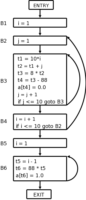
   1)  i = 1
   2)  j = 1
   3)  t1 = 10 * i
   4)  t2 = t1 + j            // element [i,j]
   5)  t3 = 8 * t2            // offset for a[i,j] (8 byte numbers)
   6)  t4 = t3 - 88           // we start at [1,1] not [0,0]
   7)  a[t4] = 0.0
   8)  j = j + 1
   9)  if J <= 10 goto (3)
  10)  i = i + 1
  11)  if i <= 10 goto (2)
  12)  i = 1
  13)  t5 = i - 1
  14)  t6 = 88 * t5
  15)  a[t6] = 1.0
  16)  i = i + 1
  17)  if i <= 10 goto (13)
Which quads are leaders?
1 is a leader by definition. The jumps are 9, 11, and 17. So 10 and 12 are leaders as are the targets 3, 2, and 13.
The leaders are then 1, 2, 3, 10, 12, and 13.
The basic blocks are {1}, {2}, {3,4,5,6,7,8,9}, {10,11}, {12}, and {13,14,15,16,17}.
Here is the code written again with the basic blocks indicated.
1) i = 12) j = 13) t1 = 10 * i 4) t2 = t1 + j // element [i,j] 5) t3 = 8 * t2 // offset for a[i,j] (8 byte numbers) 6) t4 = t3 - 88 // we start at [1,1] not [0,0] 7) a[t4] = 0.0 8) j = j + 1 9) if J <= 10 goto (3)10) i = i + 1 11) if i <= 10 goto (2)12) i = 113) t5 = i - 1 14) t6 = 88 * t5 15) a[t6] = 1.0 16) i = i + 1 17) if i <= 10 goto (13)
We can see that once you execute the leader you are assured of executing the rest of the block in order.
We want to record the flow of information from instructions that compute a value to those that use the value. One advantage we will achieve is that if we find a value has no subsequent uses, then it is dead and the register holding that value can be used for another value.
Assume that a quad p assigns a value to x (some would call this a def of x).
Definition: Another quad q uses the value computed at p (uses the def) and x is live at q if q has x as an operand and there is a possible execution path from p to q that does not pass any other def of x.
Since the flow of control is trivial inside a basic block, we are able to compute the live/dead status and next use information for at the block leader by a simple backwards scan of the quads (algorithm below).
Note that if x is dead (i.e., not live) on entrance to B the register containing x can be reused in B.
Our goal is to determine whether a block uses a value and if so in which statement.
  Initialize all variables in B as being live
  Examine the quads of the block in reverse order.
    Let the quad q compute x and read y and z
    Mark x as dead; mark y and z as live and used at q
When the loop finishes those values that are read before being are marked as live and their first use is noted. The locations x that are set before being read are marked dead meaning that the value of x on entrance is not used.
The nodes of the flow graph are the basic blocks and there is an edge from P (predecessor) to S (successor) if the last statement of P
Two nodes are added: entry
and exit
.
An edge is added from entry to the first basic block.
Edges to the exit are added from any block that could be the last block executed. Specifically edges are added from
The flow graph for our example is shown on the right.
Note that jump targets are no longer quads but blocks. The reason is that various optimizations within blocks will change the instructions and we would have to change the jump to reflect this.
Of course most of a program's execution time is within loops so we want to identify these.
Definition: A collection of basic blocks forms a loop L with loop entry E if
The flow graph on the right has three loops.
Homework: Consider the following program for matrix multiplication.
  for (i=0; i<10; i++)
      for (j=0; j<10; j++)
          c[i][j] = 0;
  for (i=0; i<10; i++)
      for (j=0; j<10; j++)
          for (k=0; k<10; k++)
              c[i][j] = c[i][j] + a[i][k] * b[k][j];