Compilers

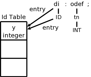
On the board, construct the parse tree, starting from the declaration for
      y = integer ;
We should get the diagram on the right.

Now let's consider arrays. We need to include td (type-definition) and tn (type-name) as well as an additional production for od (object-definition). For td we need the restriction that tn is a basic type since we cannot define higher dimensional arrays.

I put in many type checks to distinguish the array case from the scalar case; possibly some are superfluous.

Once again all attributes are synthesized (including those with side effects) so we have an S-attributed SDD.

Array Declarations

Production	Semantic Rules
d → od	d.width = od.width
d → td	d.width = 0
od → di : odef ;	addType(di.entry, odef.type) od.width = odef.width
di → ID	di.entry = ID.entry
odef → tn	odef.type = tn.type
	odef.width = tn.width
	tn.type must be integer or real
odef → tn [ NUM ]	odef.type = array(NUM.value, getBaseType(tn.entry.type)
	odef.width = sizeof(odef.type)     = NUM.value*sizeof(getBaseType(tn.entry.type))
	tn must be ID
td → TYPE di IS ARRAY OF tn ;	addType(di.entry, Array(*, tn.type))
	tn.type must be integer or real
tn → ID	tn.entry = ID.entry
	ID.entry.type must be array()
tn → INT	tn.type = integer
	tn.width = 4
tn → REAL	tn.type = real
	tn.width = 8

The top diagram on the right shows the result of applying the semantic actions in the table above to to the declaration
      type t is array of real;

The bottom diagram shows the result after
      x : t[10];

6.3.5: Sequences of Declarations

The Run Time Storage of Objects

Be careful to distinguish three methods used to store and pass information.

1. Atrributes. These are variables in a phase (semantics analyzer; also intermediate code generator) of the compiler.
2. Identifier (and other) table. This is longer lived data; often passed between phases.
3. Run time storage. This is storage established by the compiler, but not used by the compiler. It is allocated and used during run time.

To summarize, the identifier table (and others we have used) are not present when the program is run. But there must be run time storage for objects. We need to know the address each object will have during execution. Specifically, we need to know its offset from the start of the area used for object storage.

For just one object, it is trivial: the offset is zero.

Multiple Declarations

The goal is to permit multiple declarations in the same procedure (or program or function). For C/java like languages this can occur in two ways.

1. Multiple objects in a single declaration.
2. Multiple declarations in a single procedure.

In either case we need to associate with the object being declared its storage location. Specifically we include in the table entry for the object, its offset from the beginning of the current procedure. We initialize this offset at the beginning of the procedure and increment it after each object declaration.

The programming languages Ada and Pascal do not permit multiple objects in a single declaration. Both languages are of the
    object : type
school. Thus lab 3, which follows Ada, and 1e, which follows pascal, do not support multiple objects in a single declaration. C/Java certainly does permit multiple objects, but surprisingly the 2e grammar does not.

Naturally, the way to permit multiple declarations is to have a list of declarations in the natural right-recursive way. The 2e C/Java grammar has D which is a list of semicolon-separated T ID's
    D → T ID ; D | ε

The lab 3 grammar has a list of declarations (each of which ends in a semicolon). Shortening declarations to ds we have
    ds → d ds | ε

As mentioned, we need to maintain an offset, the next storage location to be used by an object declaration. The 2e snippet below introduces a nonterminal P for program that gives a convenient place to initialize offset.

    P →                { offset = 0; }
        D
    D → T ID ;         { top.put(id.lexeme, T.type, offset);
                              offset = offset + T.width; }
        D1
    D → ε
  

The name top is used to signify that we work with the top symbol table (when we have nested scopes for record definitions we need a stack of symbol tables). Top.put places the identifier into this table with its type and storage location. We then bump offset for the next variable or next declaration.

Rather that figure out how to put this snippet together with the previous 2e code that handled arrays, we will just present the snippets and put everything together on the lab 3 grammar.

In the function-def (fd) and procedure-def (pd) productions we add the inherited attribute offset to declarations (ds.offset) and set it to zero. We then inherit this offset down to an individual declaration. If this is an object declaration, we store it in the entry for the identifier being declared and we increment the offset by the size of this object. When we get the to the end of the declarations (the ε-production), the offset value is the total size needed. So we turn it around and send it back up the tree.

Multiple Declarations

Production	Semantic Rules	Kind
fd → FUNC di ( ps ) RET tn IS ds BEG s ss END ;	ds.offset = 0	Inherited
pd → PROC di ( ps ) IS ds BEG s ss END ;	ds.offset = 0	Inherited
	s.next = newlabel()	Inherited
	ss.next = newlabel()	Inherited
	pd.code = s.code || label(s.next) || ss.code || label(ss.next)	Synthesized
ds → d ds1	d.offset = ds.offset	Inherited
	ds1.offset = d.newoffset	Inherited
	ds.totalSize = ds1.totalSize	Synthesized
ds → ε	ds.totalSize = ds.offset	Synthesized
d → od	od.offset = d.offset	Inherited
	d.newoffset = d.offset + od.width	Synthesized
d → td	d.newoffset = d.offset	Synthesized
od → di : odef ;	addType(di.entry, odef.type)	Synthesized
	od.width = odef.width	Synthesized
	addOffset(di.entry, od.offset)	Synthesized
di → ID	di.entry = ID.entry	Synthesized
odef → tn	odef.type = tn.type	Synthesized
	odef.width = tn.width	Synthesized
	tn.type must be integer or real
odef → tn [ NUM ]	odef.type = array(NUM.value, getBaseType(tn.entry.type))	Synthesized
	odef.width = sizeof(odef.type)	Synthesized
	tn must be ID
td → TYPE di is ARRAY OF tn ;	addType(di.entry, array(*, tn.type))	Synthesized
	tn.type must be integer or real
tn → ID	tn.entry = ID.entry	Synthesized
	ID.entry.type must be array()
tn → INT	tn.type = integer	Synthesized
	tn.width = 4	Synthesized
tn → REAL	tn.type = real	Synthesized
	tn.width = 8	Synthesized

Now show what happens when the following program is parsed and the semantic rules above are applied.

    procedure test () is
        y : integer;
        type t is array of real;
        x : t[10];
    begin
        y = 5;        // we haven't yet done statements
        x[2] = y;     // type error?
    end;
  

6.3.6: Fields in Records and Classes

Since records can essentially have a bunch of declarations inside, we only need add
T → RECORD { D }
to get the syntax right. For the semantics we need to push the environment and offset onto stacks since the namespace inside a record is distinct from that on the outside. The width of the record itself is the final value of (the inner) offset.

    T → record {         { Env.push(top);  top = new Env()
                           Stack.puch(offset); offset = 0; }
    D }                  { T.type = record(top); T.width = offset;
                           top = Env.pop(); offset = Stack.pop(); }
  

This does not apply directly to the lab 3 grammar since the grammar does not have records. It does, however, have procedures that can be nested. If we wanted to generate code for nested procedures we would need to stack the symbol table as done here in 2e.

Homework: Determine the types and relative addresses for the identifiers in the following sequence of declarations.

   float x;
   record { float x; float y; } rec;
   float y;
 

6.4: Translation of Expressions

Remark: See 8.3 in 1e.

The goal is to generate 3-address code for expressions. We will generate them using the natural notation of 6.2. In fact we assume there is a function gen() that given the pieces needed does the proper formatting so gen(x = y + z) will output the corresponding 3-address code. gen() is often called with addresses rather than lexemes like x. The constructor Temp() produces a new address in whatever format gen needs. Hopefully this will be clear in the tables that follow

6.4.1: Operations Within Expressions

In fact, we do a little more and generate code for assignment statements.

We will use two attributes code and address. For a parse tree node the code attribute gives the three address code to evaluate the input derived from that node. In particular, code at the root performs the entire assignment statement. there.

The attribute addr at a node is the address that holds the value calculated by the code at the node. Recall that unlike real code for a real machine our 3-address code doesn't reuse addresses.

As one would expect for expressions, all the attributes in the table to the right are synthesized. The table is for the expression part of the lab 3 grammar. To save space let's use as for assignment-statement, lv for lvalue, e for expression, t for term, and f for factor. Since we will be covering arrays a little later, we do not consider LET array-element.

6.4.2: Incremental Translation

We saw this in chapter 2.

The method in the previous section generates long strings and we walk the tree. By using SDT instead of using SDD, you can output parts of the string as each node is processed.

6.4.3: Addressing Array Elements

The idea is that you associate the base address with the array name. That is, the offset stored in the identifier table is the address of the first element of the array. The indices and the array bounds are used to compute the amount, often called the offset (unfortunately, we have already used that term), by which the address of the referenced element differs from the base address.

One Dimensional Arrays

For one dimensional arrays, this is especially easy: The address increment is the width of each element times the index (assuming indexes start at 0). So the address of A[i] is the base address of A plus i times the width of each element of A.

The width of each element is the width of what we have called the base type. So for an ID the element width is sizeof(getBaseType(ID.entry.type)). For convenience we define getBaseWidth by the formula

        getBaseWidth(ID.entry) = sizeof(getBaseType(ID.entry.type))

Two Dimensional Arrays

Let us assume row major ordering. That is, the first element stored is A[0,0], then A[0,1], ... A[0,k-1], then A[1,0], ... . Modern languages use row major ordering.

With the alternative column major ordering, after A[0,0] comes A[1,0], A[2,0], ... .

For two dimensional arrays the address of A[i,j] is the sum of three terms

1. The base address of A.
2. The distance from A to the start of row i. This is i times the width of a row, which is i times the number of elements in a row times the width of an element. The number of elements in a row is the column array bound.
3. The distance from the start of row i to element A[i,j]. This is j times the width of an element.

(In some languages A[i,j] is written A[i][j].)

Higher Dimensional Arrays

The generalization to higher dimensional arrays is clear.