Compilers

Remark: See the new section Evaluating L-Attributed Definitions in section 5.2.4.

5.3: Applications of Syntax-Directed Translations

5.3.1: Construction of Syntax Trees

Production	Semantic Rules
E → E 1 + T	E.node = new Node('+',E1.node,T.node)
E → E 1 - T	E.node = new Node('-',E1.node,T.node)
E → T	E.node = T.node
T → ( E )	T.node = E.node
T → ID	T.node = new Leaf(ID,ID.entry)
T → NUM	T.node = new Leaf(NUM,NUM.val)

Recall that in a syntax tree (technically an abstract syntax tree) we just have the essentials. For example 7+3*5, would have one + node, one *, and the three numbers. Lets see how to construct the syntax tree from an SDD.

Assume we have two functions Leaf(op,val) and Node(op,c1,...,cn), that create leaves and interior nodes respectively of the syntax tree. Leaf is called for terminals. Op is the label of the node (op for operation) and val is the lexical value of the token. Node is called for nonterminals and the ci's refer (are pointers) to the children.

Production	Semantic Rules	Type
E → T E'	E.node=E'.syn	Synthesized
	E'node=T.node	Inherited
E' → + T E'1	E'1.node=new Node('+',E'.node,T.node)	Inherited
	E'.syn=E'1.syn	Synthesized
E' → - T E'1	E'1.node=new Node('-',E'.node,T.node)	Inherited
	E'.syn=E'1.syn	Synthesized
E' → ε	E'.syn=E'.node	Synthesized
T → ( E )	T.node=E.node	Synthesized
T → ID	T.node=new Leaf(ID,ID.entry)	Synthesized
T → NUM	T.node=new Leaf(NUM,NUM.val)	Synthesized

The upper table on the right shows a left-recursive grammar that is S-attributed (so all attributes are synthesized).

Try this for x-2+y and see that we get the syntax tree.

When we eliminate the left recursion, we get the lower table on the right. It is a good illustration of dependencies. Follow it through and see that you get the same syntax tree as for the left-recursive version.

Remarks:

1. In the first edition (section 8.1) we have nearly the same table. The main difference is the switch from algol/pascal-like notation (mknode) to a java/object-like new.
2. These two functions, new Node and new Leaf (or their equivalent), are needed for lab 3 (part 4), if you are doing a recursive-descent parser. When processing a production
   1. Create a parse tree node for the LHS.
   2. Call subroutines for RHS symbols and connect the resulting nodes to the node created in i.
   3. Return a reference to the new node so the parent can hook it into the parse tree.
3. It is the lack of a call to new in the third and fourth productions that causes the (abstract) syntax tree to be produced rather than the parse (concrete syntax) tree.
4. Production compilers do not produce a parse tree, but only the syntax tree. The syntax tree is smaller, and hence more (space and time) efficient for subsequent passes that walk the tree. The parse tree might be (I believe) very slightly easier to construct as you don't have to decide which nodes to produce; you simply produce them all.

5.3.2: The structure of a Type

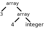
This course emphasizes top-down parsing (at least for the labs) and hence we must eliminate left recursion. The resulting grammars need inherited attributes, since operations and operands are in different productions. But sometimes the language itself demands inherited attributes. Consider two ways to describe a 3x4, two-dimensional array.

    array [3] of array [4] of int    and     int[3][4]
  

Assume that we want to produce a structure like the one the right for the array declaration given above. This structure is generated by calling a function array(num,type). Our job is to create an SDD so that the function gets called with the correct arguments.

For the first language representation of arrays (found in Ada and similar to that in lab 3), it is easy to generate an S-attributed (non-left-recursive) grammar based on
A → ARRAY [ NUM ] OF A | INT | FLOAT
This is shown in the table on the left.

Production	Semantic Rules	Type
T → B C	T.t=C.t	Synthesized
	C.b=B.t	Inherited
B → INT	B.t=integer	Synthesized
B → FLOAT	B.t=float	Synthesized
C → [ NUM ] C1	C.t=array(NUM.val,C1.t)	Synthesized
	C1.b=C.b	Inherited
C → ε	C.t=C.b	Synthesized

Production	Semantic Rule
A → ARRAY [ NUM ] OF A1	A.t=array(NUM.val,A1.t)
A → INT	A.t=integer
A → FLOAT	A.t=float

On the board draw the parse tree and see that simple synthesized attributes above suffice.

For the second language representation of arrays (the C-style), we need some smarts (and some inherited attributes) to move the int all the way to the right. Fortunately, the result, shown in the table on the right, is L-attributed and therefore all is well.

Homework: 5.6

5.4: Syntax-Directed Translation Schemes (SDTs)

Basically skipped.

The idea is that instead of the SDD approach, which requires that we build a parse tree and then perform the semantic rules in an order determined by the dependency graph, we can attach semantic actions to the grammar (as in chapter 2) and perform these actions during parsing, thus saving the construction of the parse tree.

But except for very simple languages, the tree cannot be eliminated. Modern commercial quality compilers all make multiple passes over the tree, which is actually the syntax tree (technically, the abstract syntax tree) rather than the parse tree (the concrete syntax tree).

5.4.1: Postfix Translation Schemes

If parsing is done bottom up and the SDD is S-attributed, one can generate an SDT with the actions at the end (hence, postfix). In this case the action is perform at the same time as the RHS is reduced to the LHS.

5.4.2: Parser-Stack Implementation of Postfix SDTs

Skipped.

5.4.3: SDTs with Actions Inside Productions

Skipped

5.4.4: Eliminating Left Recursion from SDTs

Skipped

5.4.5: SDTs For L-Attributed Definitions

Skipped

5.5: Implementing L-Attributed SDD's

A good summary of the available techniques.

1. Build the parse tree and annotate. Works as long as no cycles are present (guaranteed by L- or S-attributed).
2. Build the parse tree, add actions, and execute the actions in preorder. Works for any L-attributed definition. Can add actions based on the semantic rules of the SDD.
3. Translate During Recursive Descent Parsing. See below.
4. Generate Code on the Fly. Also uses recursive descent, but is restrictive.
5. Implement an SDT during LL-parsing. Skipped.
6. Implement an SDT during LR-parsing of an LL Language. Skipped.

5.5.1: Translation During Recursive-Descent Parsing

Recall that in recursive-descent parsing there is one procedure for each nonterminal. Assume the SDD is L-attributed. Pass the procedure the inherited attributes it might need (different productions with the same LHS need different attributes). The procedure keeps variables for attributes that will be needed (inherited for nonterminals in the body; synthesized for the head). Call the procedures for the nonterminals. Return all synthesized attributes for this nonterminal.

5.5.2: On-the-fly Code Generation

5.5.3: L-attributed SDDs and LL Parsing

5.5.4: Bottom-Up Parsing of L-Attributed SDDs

Requires an LL (not just LR) language.

What is this all used for?

Assume we have a parse tree as produced, for example, by your lab3. You now want to write the semantics analyzer, or intermediate code generator, and you have these semantic rules or actions that need to be performed. Assume the grammar is L-attributed, so we don't have to worry about dependence loops.

You start to write

As described in 5.5.1 above, you have received as parameters (in addition to tree-node), the attributes you are to inherit. You then call yourself recursively, with the tree-node argument set to your leftmost child, then call again using the next child, etc. Each time, you pass to the child the attributes it needs to inherit (You may be giving it too many since you know the nonterminal represented by this child but not the production; you could find out the production by examining the child's children, but probably don't bother doing so.)

When each child returns, it supplies as its return value the synthesized attributes it is passing back to you.

After the last child returns, you return to your caller, passing back the synthesized attributes you are to calculate.

Variations

1. Instead of a giant switch, you could have separate routines for each nonterminal as done in the parser and just switch on the productions having this nonterminal as LHS.
2. You could have separate routines for each production (requires looking 2-deep, as mentioned above).
3. If you like actions instead of rules, perform the actions where indicated in the SDT.
4. Global variable can be used (with care) instead of parameters.
5. As illustrated earlier in the notes, you can call routines instead of setting an attribute (see addType in 5.2.5).

Chapter 6: Intermediate-Code Generation

Remark: This corresponds to chapters 6 and 8 in the first edition. The change is that storage management is now done after intermediate code generation.

Homework: Read Chapters 6 and 8.

6.1: Variants of Syntax Trees

Remark: This is 8.1 in 1e.

6.1.1: Directed Acyclic Graphs for Expressions

The difference between a syntax DAG and a syntax tree is that the former can have undirected cycles. DAGs are useful where there are multiple, identical portions in a given input. The common case of this is for expressions where there often are common subexpressions. For example in the expression
X + a + b + c - X + ( a + b + c )
each individual variable is a common subexpression. But a+b+c is not since the first occurrence has the X already added. This is a real difference when one considers the possibility of overflow or of loss of precision. The easy case is
x + y * z * w - ( q + y * z * w )
where y*z*w is a common subexpression.

It is easy to find these. The constructor Node() above checks if an identical node exists before creating a new one. So Node ('/',left,right) first checks if there is a node with op='/' and children left and right. If so, a reference to that node is returned; if not, a new node is created as before.

Homework: Construct the DAG for
((x+y)-((x+y)*(x-y)))+((x+y)*(x-y))

6.1.2: The Value-Number Method for Constructing DAGS

Often one stores the tree or DAG in an array, one entry per node. Then references to the array index of a node is called the node's value-number. Searching an unordered array is slow; there are many better data structures to use. Hash tables are a good choice.

6.2: Three-Address Code

Instructions of the form op a,b,c, where op is a primitive operator. For example

    lshift a,b,4   // left shift b by 4 and place result in a
    add    a,b,c   // a = b + c
    a = b + c      // alternate (more natural) representation of above
  

If we are starting with a DAG (or syntax tree if less aggressive), then transforming into 3-address code is just a topological sort and an assignment of a 3-address operation with a new name for the result to each interior node (the leaves already have names and values).

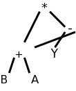
For example, (B+A)*(Y-(B+A)) produces the DAG on the right, which yields the following 3-address code.

    t1 = B + A
    t2 = Y - t1
    t3 = t1 * t2
  

6.2.1: Addresses and Instructions

We use the term 3-address when we view the (intermediate-) code as having one elementary operation with three operands, each of which is an address. Typically two of the addresses represent source operands or arguments of the operation and the third represents the result. Some of the 3-address operations have fewer than three addresses; we simply think of the missing addresses as unused (or ignored) fields in the instruction.

Possible addresses

1. (Source program) Names. Really the intermediate code would contain a reference to the (identifier) table entry for the name. For convenience, the actually identifier is often written.
2. Constants. Again, this would often be a reference to a table entry. An important issue is type conversion that will be discussed later. Type conversion also applies to identifiers.
3. (Compiler-generated) Temporaries. Although it may at first seem wasteful, modern practice assigns a new name to each temporary, rather than reusing the same temporary. (Remember that a DAG node is considered one temporary even if it has many parents.) Later phases can combine several temporaries into one (e.g., if they have disjoint lifetimes).

Possible three-address instructions

There is no universally agreed to set of three-address instructions or to whether 3-address code should be the intermediate code for the compiler. Some prefer a set close to a machine architecture. Others prefer a higher-level set closer to the source, for example, subsets of C have been used. Others prefer to have multiple levels of intermediate code in the compiler with one phase of compilation being converting from the high-level intermediate code into the low-level intermediate code. What follows is the set proposed in the 2ed; it looks to be essentially the same as that in the 1e.

In the list below, x, y, and z are addresses, i is an integer, and L is a symbolic label, as used in chapter 2. The instructions can be thought of as numbered and the labels can be converted to the numbers with another pass over the output or via backpatching, which is discussed below.

1. Binary ops. x = y op z
2. Unary ops. x = op y (includes copy, where op is the identity f(x)=x)
3. Junp. goto L.
4. Conditional unary op jumps. if x goto L   ifFalse x goto L.
5. Conditional binary op jumps. if x relop y goto L
6. Procedure/Function Calls and Returns.
     param x     call p,n     y = call p,n     return     return y.
7. Indexed Copy ops. x = y[i]   x[i] = y.
8. Address and pointer ops. x = &y   x = *y   *x

Homework: 8.1

6.2.2: Quadruples (Quads)

An easy way to represent the three address instructions: put the op into the first of four fields and the addresses into the remaining three. Some instructions do not use all the fields. Many operands will be references to entries in tables (e.g., the identifier table).

6.2.3: (Indirect) Triples

Optimization to save a field. The result field of a quad is omitted in a triple since the result is often a temporary.

When this result occurs as a source operand of a subsequent instruction, we indicate it by writing the value-number of the first instruction (distinguished some way, say with parens) as the operand of the second.

If the result field of a quad is not a temporary then two triples may be needed: One to do the operation and place the result into a temporary (which is not a field of the instruction). The second operation is a copy operation from the temporary to the final home. Recall that a copy does not use all the fields of a quad no fits into a triple without omitting the result.

When an optimizing compiler reorders instructions for increased performance, extra work is needed with triples since the instruction numbers, which have changed, are used implicitly. Hence the triples must be regenerated with correct numbers as operands.

Indirect triples. Keep an array of pointers to triples and, if it is necessary to reorder instructions, just reorder these pointers. This has two advantages.

1. The pointers are (probably) smaller than the triples so faster to move. This is a generic advantage and could be used for quads and many other reordering applications (e.g., sorting large records).
2. Since the triples don't move, the references they contain to past results remain accurate. This is specific to triples (or similar situations).

Homework: 8.2

6.2.4: Static Single-Assignment (SSA) Form

This has become a big deal in modern optimizers, but we will largely ignore it. The idea is that you have all assignments go to unique (temporary) variables. So if the code is
if x then y=4 else y=5
it is treated as though it was
if x then y1=4 else y2=5
The interesting part comes when y is used later in the program and the compiler must choose between y1 and y2.

6.3: Types and Declarations

Much of the early part of this section is really programming languages. In 1e this is section 6.1 (back from chapter 8).

6.3.1: Type Expressions

A type expression is either a basic type or the result of applying a type constructor.

6.3.2: Type Equivalence

There are two camps, name equivalence and structural equivalence.

Consider the following for example.

    declare
       type MyInteger is new Integer;
       MyX : MyInteger;
       x   : Integer := 0;
    begin
       MyX := x;
    end
  

When you have an object of an anonymous type as in
    x : array [5] of integer;
it doesn't have the same type as any other object even
    y : array [5] of integer;
But x[2] has the same type as y[3]; both are integers.

6.3.3: Declarations

The following from 2ed uses C/Java array notation. The 1ed has pascal-like material (section 6.2). Although I prefer Ada-like constructs as in lab 3, I realize that the class knows C/Java best so like the authors I will go with the 2ed. I will try to give lab3-like grammars as well.

This grammar gives C/Java like records/structs/methodless-classes as well as multidimensional arrays (really arrays of arrays).

    D → T id ; D | ε
    T → B C | RECORD { D }
    B → INT | FLOAT
    C → [ NUM ] C | ε
  

The lab 3 grammar doesn't support records and the support for multidimensional arrays is flawed (you can define the type, but not a (constrained) object). Here is the part of the lab3 grammar that handles declarations of ints, reals and arrays.

    declarations         → declaration declarations | ε
    declaration          → object-declaration | type-declaration
    object-declaration   → defining-identifier : object-definition ;
    object-definition    → type-name | type-name [ NUMBER ]
    type-declaration     → TYPE defining-identifier IS ARRAY OF type-name ;
    defining-identifier  → IDENTIFIER
    type-name            → IDENTIFIER | INT | REAL
  

    ds   → d ds | ε
    d    → od | td
    od   → di : odef ;
    odef → tn | tn [ NUM ]
    td   → TYPE di IS ARRAY OF tn ;
    di   → ID
    tn   → ID | INT | REAL
  

Ada Constrained vs Unconstrained Array Types (unofficial)

Ada supports both constrained array types such as
    type t1 is array [5] of integer
and unconstrained array types (as in lab 3) such as
    type t2 is array of integer
With the latter, the constraint is specified when the array (object) itself is declared.
    x1 : t1
    x2 : t2[5]
The grammar in lab3 supports t2 and x2, but not t1 and x1. The deficiency of the lab3 grammar is that for two dimensional array types
    type t3 is array of t2
we have no way to supply the two array bounds in the array (object) definition. Ada, which as said above, has both constrained and unconstrained array types, forbids the latter from appearing after is array of.

You might wonder why we want the unconstrained type. These types permit a procedure to have a parameter that is an array of integers of unspecified size. Remember that the declaration of a procedure specifies only the type of the parameter; the object is determined at the time of the procedure call.

6.3.4: Storage Layout for Local Names

See section 8.2 in 1e (we are going back to chapter 8 from 6, so perhaps Doc Brown from BTTF should give the lecture).

We are considering here only those types for which the storage can be computed at compile time. For others, e.g., string variables, dynamic arrays, etc, we would only be reserving space for a pointer to the structure; the structure itself is created at run time and is discussed in the next chapter.

The idea is that the basic type determines the width of the data, and the size of an array determines the height. These are then multiplied to get the size (area) of the data.

The book uses semantic actions (i.e., a syntax directed translation SDT). I added the corresponding semantic rules so that we have an SDD as well.

Remember that for an SDT, the placement of the actions withing the production is important. Since it aids reading to have the actions lined up in a column, we sometimes write the production itself on multiple lines. For example the production T→BC has the B and C on separate lines so that the action can be in between even though it is written to the right of both.

The actions use global variables t and w to carry the base type (INT or FLOAT) and width down to the ε-production, where they are then sent on their way up and become multiplied by the various dimensions. In the rules I use inherited attributes bt and bw. This is similar to the comment above that instead of having the identifier table passed up and down via attributes, the bullet is bitten and a globally visible table is used.

The base types and widths are set by the lexer or are constants in the parser.

Using the Lab 3 Grammar

First let's ignore arrays. Then we get the simple table on the right. All the attributes are Synthesized so we have an S-attributed grammar.

We dutifully synthesize the width attribute all the way to the top and then do not use it. We shall use it in the next section when we consider multiple declarations.

Recall that addType is viewed as a synthesized since its parameters come from the RHS, i.e., from children of this node. It has a side effect (of modifying the identifier table) so we must be sure that we are not depending on some order of evaluation that is not simply parent after children. In fact, later when we evaluate expressions, we will need some of this information. We will need to enforce declaration before use since we will be looking up information that we are setting here. So in evaluation, we check the entry in the identifier table to be sure that the type (for example) has already been set.

Note the comment tn.type must be integer or real. This is an example of a type check, a key component of semantic analysis, that we will learn about soon. The reason for it here is that we are only able to handle 1 dimensional arrays with the lab3 grammar. (It would be a more complicated grammar with other type check rules to handle the general case found in ada).