================ Start Lecture #7 ================
Say I is a set of items and one of these items is A→α·Bβ. This item represents the parser having seen α and records that the parser might soon see the remainder of the RHS. For that to happen the parser must first see a string derivable from B. Now consider any production starting with B, say B→γ. If the parser is to making progress on A→α·Bβ, it will need to be making progress on one such B→·γ. Hence we want to add all the latter productions to any state that contains the former. We formalize this into the notion of closure.
Definition: For any set of items I, CLOSURE(I) is formed as follows.
Example: Recall our main example
   E' → E
    E → E + T | T
    T → T * F | F
    F → ( E ) | id
CLOSURE({E' → E})
contains 7 elements.
The 6 new elements are the 6 original productions each with a dot
right after the arrow.
If X is a grammar symbol, then moving from A→α·Xβ to A→αX·β signifies that the parser has just processed (input derivable from) X. The parser was in the former position and X was on the input; this caused the parser to go to the latter position. We (almost) indicate this by writing GOTO(A→α·Xβ,X) is A→αX·β. I said almost because GOTO is actually defined from item sets to item sets not from items to items.
Definition: If I is an item set and X is a grammar symbol, then GOTO(I,X) is the closure of the set of items A→αX·β where A→α·Xβ is in I.
I really believe this is very clear, but I understand that the formalism makes it seem confusing. Let me begin with the idea.
We augment the grammar and get this one new production; take its closure. That is the first element of the collection; call it Z. Try GOTOing from Z, i.e., for each grammar symbol, consider GOTO(Z,X); each of these (almost) is another element of the collection. Now try GOTOing from each of these new elements of the collection, etc. Start with jane smith, add all her friends F, then add the friends of everyone in F, called FF, then add all the friends of everyone in FF, etc
The (almost)
is because GOTO(Z,X) could be empty so formally
we construct the canonical collection of LR(0) items, C, as follows
This GOTO gives exactly the arcs in the DFA I constructed earlier. The formal treatment does not include the NFA, but works with the DFA from the beginning.
Homework:
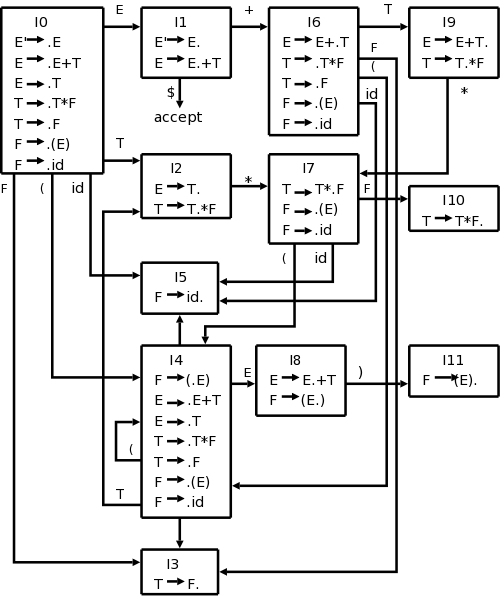
Our main example is larger than the toy I did before. The NFA would have 2+4+2+4+2+4+2=20 states (a production with k symbols on the RHS gives k+1 N-states since there k+1 places to place the dot). This gives rise to 11 D-states. However, the development in the book, which we are following now, constructs the DFA directly. The resulting diagram is on the right.
Start constructing the diagram on the board. Begin with {E' → ·E}, take the closure, and then keep applying GOTO.
The LR-parsing algorithm must decide when to shift and when to reduce (and in the latter case, by which production). It does this by consulting two tables, ACTION and GOTO. The basic algorithm is the same for all LR parsers, what changes are the tables ACTION and GOTO.
We have already seen GOTO (for SLR).
Technical point that may, and probably should, be ignored: our GOTO was defined on pairs [item-set,grammar-symbol]. The new GOTO is defined on pairs [state,nonterminal]. A state (except the initial state) is an item set together with the grammar symbol that was used to generate it (via the old GOTO). We will not use the new GOTO on terminals so we just define it on nonterminals.
Given a state i and a terminal a (or the endmarker), ACTION[i,a] can be
So ACTION is the key to deciding shift vs. reduce. We will soon see how this table is computed for SLR.
Since ACTION is defined on [state,terminal] pairs and GOTO is defined on [state,nonterminal], we can combine these tables into one defined on [state,grammar-symbol] pairs.
This formalism is useful for stating the actions of the parser precisely, but I believe it can be explained without it.
As mentioned above the Symbols column is redundant so a configuration of the parser consists of the current stack and the remainder of the input. Formally it is
The parser consults the combined ACTION-GOTO table for its current state (TOS) and next input symbol, formally this is ACTION[sm,ai], and proceeds as follows based on the value in the table. We have done this informally just above; here we use the formal treatment
The missing piece of the puzzle is finally revealed.
The book (both editions) and the rest of the world seem to use GOTO for both the function defined on item sets and the derived function on states. As a result we will be defining GOTO in terms of GOTO. (I notice that the first edition uses goto for both; I have been following the second edition, which uses GOTO. I don't think this is a real problem.) Item sets are denoted by I or Ij, etc. States are denoted by s or si or (get ready) i. Indeed both books use i in this section. The advantage is that on the stack we placed integers (i.e., i's) so this is consistent. The disadvantage is that we are defining GOTO(i,A) in terms of GOTO(Ii,A), which looks confusing. Actually, we view the old GOTO as a function and the new one as an array (mathematically, they are the same) so we actually write GOTO(i,A) and GOTO[Ii,A].
We start with an augmented grammar (i.e., we added S' → S).
shift j, where GOTO(Ii,b)=Ij.
reduce A→α.
accept.
error.
| State | ACTION | GOTO | |||||||
|---|---|---|---|---|---|---|---|---|---|
| id | + | * | ( | ) | $ | E | T | F | |
| 0 | s5 | s4 | 1 | 2 | 3 | ||||
| 1 | s6 | acc | |||||||
| 2 | r2 | s7 | r2 | r2 | |||||
| 3 | r4 | r4 | r4 | r4 | |||||
| 4 | s5 | s4 | 8 | 2 | 3 | ||||
| 5 | r6 | r6 | r6 | r6 | |||||
| 6 | s5 | s4 | 9 | 3 | |||||
| 7 | s5 | s4 | 10 | ||||||
| 8 | s6 | s11 | |||||||
| 9 | r1 | s7 | r1 | r1 | |||||
| 10 | r3 | r3 | r3 | r3 | |||||
| 11 | r5 | r5 | r5 | r5 | |||||
shift and go to state 5.
reduce by production number 2, where we have numbered the productions as follows.
The shift actions can be read directly off the DFA. For example I1 with a + goes to I6, I6 with an id goes to I5, and I9 with a * goes to I7.
The reduce actions require FOLLOW.
Consider I5={F→id·}.
Since the dot is at the end, we are ready to reduce, but we must
check if the next symbol can follow the F we are reducing to.
Since FOLLOW(F)={+,*,),$}, in row 5 (for I5) we put
r6 (for reduce by production 6
) in the columns for
+, *, ), and $.
The GOTO columns can also be read directly off the DFA. Since there is an E-transition (arc labeled E) from I0 to I1, the column labeled E in row 0 contains a 1.
Since the column labeled + is blank for row 7, we see that it would be an error if we arrived in state 7 when the next input character is +.
Finally, if we are in state 1 when the input is exhausted ($ is the next input character), then we have a successfully parsed the input.
| Stack | Symbols | Input | Action |
|---|---|---|---|
| 0 | id*id+id$ | shift | |
| 05 | id | *id+id$ | reduce by F→id |
| 03 | F | *id+id$ | reduct by T→id |
| 02 | T | *id+id$ | shift |
| 027 | T* | id+id$ | shift |
| 0275 | T*id | +id$ | reduce by F→id |
| 027 10 | T*F | +id$ | reduce by T→T*F |
| 02 | T | +id$ | reduce by E→T |
| 01 | E | +id$ | shift |
| 016 | E+ | id$ | shift |
| 0165 | E+id | $ | reduce by F→id |
| 0163 | E+F | $ | reduce by T→F |
| 0169 | E+T | $ | reduce by E→E+T |
| 01 | E | $ | accept |
Homework:
Construct the SLR parsing table for the
following grammar
X → S S + | S S * | a
You already constructed the LR(0) automaton for this example in
the previous homework.
Skipped.
We consider very briefly two alternatives to SLR, canonical-LR or LR, and lookahead-LR or LALR.
SLR used the LR(0) items, that is the items used were productions with an embedded dot, but contained no other (lookahead) information. The LR(1) items contain the same productions with embedded dots, but add a second component, which is a terminal (or $). This second component becomes important only when the dot is at the extreme right (indicating that a reduction can be made if the input symbol is in the appropriate FOLLOW set). For LR(1) we do that reduction only if the input symbol is exactly the second component of the item. This finer control of when to perform reductions, enables the parsing of a larger class of languages.
Skipped.
Skipped.
For LALR we merge various LR(1) item sets together, obtaining nearly the LR(0) item sets we used in SLR. LR(1) items have two components, the first, called the core, is a production with a dot; the second a terminal. For LALR we merge all the item sets that have the same cores by combining the 2nd components (thus permitting reductions when any of these terminals is the next input symbol). Thus we obtain the same number of states (item sets) as in SLR since only the cores distinguish item sets.
Unlike SLR, we limit reductions to occurring only for certain specified input symbols. LR(1) gives finer control; it is possible for the LALR merger to have reduce-reduce conflicts when the LR(1) items on which it is based is conflict free.
Although these conflicts are possible, they are rare and the size reduction from LR(1) to LALR is quite large. LALR is the current method of choice for bottom-up, shift-reduce parsing.
Skipped.
Skipped.
Skipped.
Dangling-ElseAmbiguity
Skipped.
Skipped.
The tool corresponding to Lex for parsing is yacc, which (at least originally) stood for yet another compiler compiler. This name is cute but somewhat misleading since yacc (like the previous compiler compilers) does not produce a compiler, just a parser.
The structure of the user input is similar to that for lex, but instead of regular definitions, one includes productions with semantic actions.
There are ways to specify associativity and precedence of operators. It is not done with multiple grammar symbols as in a pure parser, but more like declarations.
Use of Yacc requires a serious session with its manual.
Skipped.
Skipped
Skipped
Homework: Read Chapter 5.
Again we are redoing, more formally and completely, things we briefly discussed when breezing over chapter 2.
Recall that a syntax-directed definition (SDD) adds semantic rules
to the productions of a grammar.
For example to the production T → T1 / F we might add the rule
T.code = T1.code || F.code || '/'
if we were doing an infix to postfix translator.
Rather than constantly copying ever larger strings to finally
output at the root of the tree after a depth first traversal, we can
perform the output incrementally by embedding semantic actions
within the productions themselves.
The above example becomes
T → T1 / F { print '/' }
Since we are generating postfix, the action comes at the end (after
we have generated the subtrees for T1 and F, and hence
performed their actions).
In general the actions occur within the production, not necessarily
after the last symbol.
For SDD's we conceptually need to have the entire tree available after the parse so that we can run the depth first traversal. (It is depth first since we are doing postfix; we will see other orders shortly.) Semantic actions can be performed during the parse, without saving the tree.
Formally, attributes are values (of any type) that are associated with grammar symbols. Write X.a for the attribute a of symbol X. You can think of attributes as fields in a record/struct/object.
Semantic rules (rules for short) are associated with productions.
Terminals can have synthesized attributes, that are given to it by the lexer (not the parser). There are no rules in an SDD giving values to attributes for terminals. Terminals do not have inherited attributes. A nonterminal A can have both inherited and synthesized attributes. The difference is how they are computed by rules associated with a production at a node N of the parse tree. We sometimes refer to the production at node N as production N.
The arithmetic division example above was synthesized.
| Production | Semantic Rules |
|---|---|
| L → E $ | L.val = E.val |
| E → E1 + T | E.val = E1.val + T.val |
| E → E1 - T | E.val = E1.val - T.val |
| E → T | E.val = T.val |
| T → T1 * F | T.val = T1.val * F.val |
| T → T1 / F | T.val = T1.val / F.val |
| T → F | T.val = F.val |
| F → ( E ) | F.val = E.val |
| F → num | F.val = num.lexval |
Example: The SDD at the right gives a left-recursive grammar for expressions with an extra nonterminal L added as the start symbol. The terminal num is given a value by the lexer, which corresponds to the value stored in the numbers table for lab 2.
Draw the parse tree for 7+6/3 on the board and verify that L.val is 9, the value of the expression.
Definition: This example use only synthesized attributes; such SDDs are called S-attributed and have the property that the rules give the attribute of the LHS in terms of attributes of the RHS.
Inherited attributes are more complicated since the node N of the parse tree with which it is associated (which is also the natural node to store the value) does not contain the production with the corresponding semantic rule.
Definition: An inherited attribute of a nonterminal B at node N (where B is the LHS) is defined by a semantic rule of the production at the parent of N (where B occurs in the RHS). The value depends only on attributes at N, N's siblings, and N's parent.
Note that when viewed from the parent node P (the site of the semantic rule), the inherited attribute depends on values at P and at P's children (the same as for synthesized attributes). However, and this is crucial, the nonterminal B is the LHS of a child of P and hence the attribute is naturally associated with that child. It is possibly stored there and is shown there in the diagrams below.
We will see an example with inherited attributes soon.
Definition:Often the attributes are just evaluations without side effects. In such cases we call the SDD an attribute grammar.