Compilers

Remark: If you find a particular homework question challenging, ask on the mailing list and an answer will be produced.

Remark: I forgot to assign homework for section 3.6. I have added one problem spread into three parts. It is not assigned but it is a question I believe you should be able to do.

3.7.1: Converting an NFA to a DFA

(This is item #3 above and is done in section 3.6 in the first edition.)

The book gives a detailed proof; I am just trying to motivate the ideas.

Let N be an NFA, we construct a DFA D that accepts the same strings as N does. Call a state of N an N-state, and call a state of D a D-state.

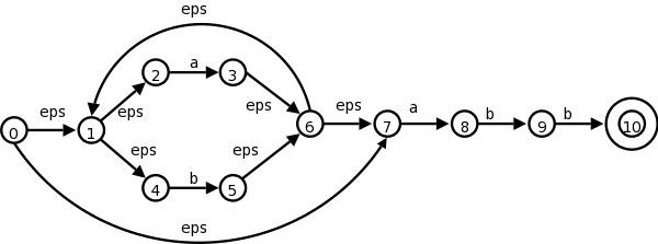
The idea is that D-state corresponds to a set of N-states and hence this is called the subset algorithm. Specifically for each string X of symbols we consider all the N-states that can result when N processes X. This set of N-states is a D-state. Let us consider the transition graph on the right, which is an NFA that accepts strings satisfying the regular expression
(a|b)^*abb.

NFA states	DFA state	a	b
{0,1,2,4,7}	D0	D1	D2
{1,2,3,4,6,7,8}	D1	D1	D3
{1,2,4,5,6,7}	D2	D1	D2
{1,2,4,5,6,7,9}	D3	D1	D4
{1,2,3,5,6,7,10}	D4	D1	D2

The start state of D is the set of N-states that can result when N processes the empty string ε. This is called the ε-closure of the start state s₀ of N, and consists of those N-states that can be reached from s₀ by following edges labeled with ε. Specifically it is the set {0,1,2,4,7} of N-states. We call this state D₀ and enter it in the transition table we are building for D on the right.

Next we want the a-successor of D₀, i.e., the D-state that occurs when we start at D₀ and move along an edge labeled a. We call this successor D₁. Since D₀ consists of the N-states corresponding to ε, D₁ is the N-states corresponding to εa=a. We compute the a-successor of all the N-states in D₀ and then form the ε-closure.

Next we compute the b-successor of D₀ the same way and call it D₂.

We continue forming a- and b-successors of all the D-states until no new D-states result (there is only a finite number of subsets of all the N-states so this process does indeed stop).

This gives the table on the right. D₄ is the only D-accepting state as it is the only D-state containing the (only) N-accepting state 10.

Theoretically, this algorithm is awful since for a set with k elements, there are 2^k subsets. Fortunately, normally only a small fraction of the possible subsets occur in practice.

Homework: Convert the NFA from the homework for section 3.6 to a DFA.

3.7.2: Simulating an NFA

Instead of producing the DFA, we can run the subset algorithm as a simulation itself. This is item #2 in my list of techniques

  S = ε-closure(s0);
  c = nextChar();
  while ( c != eof ) {
    S = ε-closure(move(S,c));
    c = nextChar();
  }
  if ( S ∩ F != φ ) return yes;   // F is accepting states
  else return no;

3.7.3: Efficiency of NFA Simulation

Slick implementation.

3.7.4: Constructing an NFA from a Regular Expression

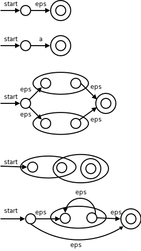
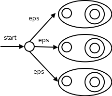
I give a pictorial proof by induction. This is item #1 from my list of techniques.

1. The base cases are the empty regular expression and the regular expression consisting of a single symbol a in the alphabet.
2. The inductive cases are.
   1. s | t for s and t regular expressions
   2. st for s and t regular expressions
   3. s^*
   4. (s), which is trivial since the nfa for s works for (s).

The pictures on the right illustrate the base and inductive cases.

Remarks:

1. The generated NFA has at most twice as many states as there are operators and operands in the RE. This is important for studying the complexity of the NFA.
2. The generated NFA has one start and one accepting state. The accepting state has no outgoing arcs and the start state has no incoming arcs.
3. Note that the diagram for st correctly indicates that the final state of s and the initial state of t are merged. This uses the previous remark that there is only one start and final state.
4. Except for the accepting state, each state of the generated NFA has either one outgoing arc labeled with a symbol or two outgoing arcs labeled with ε.

Do the NFA for (a|b)^*abb and see that we get the same diagram that we had before.

Do the steps in the normal leftmost, innermost order (or draw a normal parse tree and follow it).

Homework: 3.16 a,b,c

3.7.5: Efficiency of String-Processing Algorithms

(This is on page 127 of the first edition.) Skipped.

3.8: Design of a Lexical-Analyzer Generator

How lexer-generators like Lex work.

3.8.1: The structure of the generated analyzer

We have seen simulators for DFAs and NFAs.

The remaining large question is how is the lex input converted into one of these automatons.

Also

1. Lex permits functions to be passed through to the yy.lex.c file. This is fairly straightforward to implement.
2. Lex also supports actions that are to be invoked by the simulator when a match occurs. This is also fairly straight forward.
3. The lookahead operator is not so simple in the general case and is discussed briefly below.

In this section we will use transition graphs, lexer-generators do not draw pictures; instead they use the equivalent transition tables.

Recall that the regular definitions in Lex are mere conveniences that can easily be converted to REs and hence we need only convert REs into an FSA.

We already know how to convert a single RE into an NFA. But lex input will contain several REs (since it wishes to recognize several different tokens). The solution is to

1. Produce an NFA for each RE.
2. Introduce a new start state.
3. Introduce an ε transition from the new start state to the start of each NFA constructed in step 1.
4. When one reaches one of the accepting states,they do NOT stop. See below for an explanation.

At each of the accepting states (one for each NFA in step 1), the simulator executes the actions specified in the lex program for the corresponding pattern.

3.8.2: Pattern Matching Based on NFAs

We use the algorithm for simulating NFAs presented in 3.7.2.

The simulator starts reading characters and calculates the set of states it is at.

At some point the input character does not lead to any state or we have reached the eof. Since we wish to find the longest lexeme matching the pattern we proceed backwards from the current point (where there was no state) until we reach an accepting state (i.e., the set of NFA states, N-states, contains an accepting N-state). Each accepting N-state corresponds to a matched pattern. The lex rule is that if a lexeme matches multiple patterns we choose the pattern listed first in the lex-program.

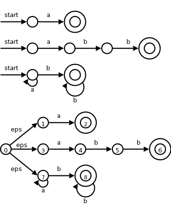
Pattern	Action to perform
a	Action1
abb	Action2
a*b+	Action3

Example

Consider the example on the right with three patterns and their associated actions and consider processing the input aaba.

1. We begin by constructing the three NFAs. To save space, the third NFA is not the one that would be constructed by our algorithm, but is an equivalent smaller one. For example, some unnecessary ε-transitions have been eliminated. If one view the lex executable as a compiler transforming lex source into NFAs, this would be considered an optimization.
2. We introduce a new start state and ε-transitions as in the previous section.
3. We start at the ε-closure of the start state, which is {0,1,3,7}.
4. The first a (remember the input is aaba) takes us to {2,4,7}. This includes an accepting state and indeed we have matched the first patten. However, we do not stop since we may find a longer match.
5. The next a takes us to {7}.
6. The b takes us to {8}.
7. The next a fails since there are no a-transitions out of state 8. So we must back up to before trying the last a.
8. We are back in {8} and ask if one of these N-states (I know there is only one, but there could be more) is an accepting state.
9. Indeed state 8 is accepting for third pattern. If there were more than one accepting state in the list, we would choose the one in the earliest listed pattern.
10. Action3 would now be performed.

3.8.3: DFA's for Lexical Analyzers

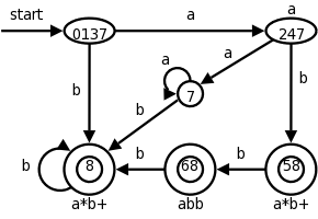
We label the accepting states with the pattern matched. If multiple patterns are matched (because the accepting D-state contains multiple accepting N-states), we use the first pattern listed (assuming we are using lex conventions).

Technical point. For a DFA, there must be a outgoing edge from each D-state for each possible character. In the diagram, when there is no NFA state possible, we do not show the edge. Technically we should show these edges, all of which lead to the same D-state, called the dead state, and corresponds to the empty subset of N-states.

3.8.4: Implementing the Lookahead Operator

This has some tricky points. Recall that this lookahead operator is for when you must look further down the input but the extra characters matched are not part of the lexeme. We write the pattern r1/r2. In the NFA we match r1 then treat the / as an ε and then match s1. It would be fairly easy to describe the situation when the NFA has only ε-transition at the state where r1 is matched. But it is tricky when there are more than one such transition.

3.9: Optimization of DFA-Based Pattern Matchers

Skipped

3.9.1: Important States of an NFA

Skipped

3.9.2: Functions Computed form the Syntax Tree

Skipped

3.9.3: Computing nullable, firstpos, and lastpos

Skipped

3.9.4: Computing followpos

Skipped

Chapter 4: Syntax Analysis

Homework: Read Chapter 4.

4.1: Introduction

4.1.1: The role of the parser

Conceptually, the parser accepts a sequence of tokens and produces a parse tree.

As we saw in the previous chapter the parser calls the lexer to obtain the next token. In practice this might not occur.

1. The source program might have errors.
2. Instead of explicitly constructing the parse tree, the actions that the downstream components of the front end would do on the tree can be integrated with the parser and done incrementally on components of the tree.

There are three classes for grammar-based parsers.

1. universal
2. top-down
3. bottom-up

The universal parsers are not used in practice as they are inefficient.

As expected, top-down parsers start from the root of the tree and proceed downward; whereas, bottom-up parsers start from the leaves and proceed upward.

The commonly used top-down and bottom parsers are not universal. That is, there are grammars that cannot be used with them.

The LL and LR parsers are important in practice. Hand written parsers are often LL. Specifically, the predictive parsers we looked at in chapter two are for LL grammars.

The LR grammars form a larger class. Parsers for this class are usually constructed with the aid of automatic tools.

4.1.2: Representative Grammars

Expressions with + and *

    E → E + T | T
    T → T * F | F
    F → ( E ) | id
  

This takes care of precedence, but as we saw before, gives us trouble since it is left-recursive and we did top-down parsing. So we use the following non-left-recursive grammar that generates the same language.

    E  → T E'
    E' → + T E' | ε
    T  → F T'
    T' → * F T' | ε
    F  → ( E ) | id
  

The following ambiguous grammar will be used for illustration, but in general we try to avoid ambiguity. This grammar does not enforce precedence.

    E → E + E | E * E | ( E ) | id
  

4.1.3: Syntax Error Handling

There are different levels of errors.

1. Lexical errors: For example, spelling.
2. Syntactic errors: For example missing ; .
3. Semantic errors: For example wrong number of array indexes.
4. Logical errors: For example off by one usage of < instead of <=.

4.1.4: Error-Recovery Strategies

The goals are clear, but difficult.

• Report errors clearly and accurately. One difficulty is that one error can mask another and can cause correct code to look faulty.
• Recover quickly enough to not miss other errors.
• Add minimal overhead.

Trivial Approach: No Recovery

Print an error message when parsing cannot continue and then terminate parsing.

Panic-Mode Recovery

The first level improvement. The parser discards input until it encounters a synchronizing token. These tokens are chosen so that the parser can make a fresh beginning. Good examples are ; and }.

Phrase-Level Recovery

Locally replace some prefix of the remaining input by some string. Simple cases are exchanging ; with , and = with ==. Difficulty is when real error occurred long before the error was detected.

Error Productions

Include productions for common errors.

Global Correction

Change the input I to the closest correct input I' and produce the parse tree for I'.

4.2: Context-Free Grammars

4.2.1: Formal Definition

1. Terminals: The basic components found by the lexer. They are sometimes called token names, i.e., the first component of the token as produced by the lexer.
2. Nonterminals: Syntactic variables that help define the syntactic structure of the language.
3. Start Symbol: A start symbol that is the root of the parse tree.
4. Productions:
   1. Head or left (hand) side or LHS. A single nonterminal.
   2. →
   3. Body or right (hand) side or RHS. A string of terminals and nonterminals.

4.2.2: Notational Conventions

I don't use these without saying so.

4.2.3: Derivations

This is mostly (very useful) notation.

Assume we have a production A → α. We would then say that A derives α and write
A ⇒ α

We generalize this. If, in addition, β and γ are strings, we say that βAγ derives βαγ and write
βAγ ⇒ βαγ

We generalize further. If x derives y and y derives z, we say x derives z and write
x ⇒* z.

The notation used is ⇒ with a * over it (I don't see it in html). This should be read derives in zero or more steps. Formally,

1. x ⇒* x, for any string x.
2. If x ⇒* y and y ⇒ z, then x ⇒* z.

Definition: If S is the start symbol and S ⇒* x, we say x is a sentential form of the grammar.

A sentential form may contain nonterminals and terminals. If it contains only terminals it is a sentence of the grammar and the language generated by a grammar G, written L(G), is the set of sentences.

Definition: A language generated by a (context-free) grammar is called a context free language.

Definition: Two grammars generating the same language are called equivalent.

Examples: Recall the ambiguous grammar above

    E → E + E | E * E | ( E ) | id
  

    E ⇒ E + E ⇒ id + E ⇒ id + id
    E ⇒ E + E ⇒ E + id ⇒ id + id
  

In the first derivation, we replaced the leftmost nonterminal by the body of a production having the nonterminal as head. This is called a leftmost derivation. Similarly the second derivation in which the rightmost nonterminal is replaced is called a rightmost derivation or a canonical derivation.

When one wishes to emphasize that a (one step) derivation is leftmost they write an lm under the ⇒. To emphasize that a (general) derivation is leftmost, one writes an lm under the ⇒*. Similarly one writes rm to indicate that a derivation is rightmost. I won't do this in the notes but will on the board.

Definition: If x can be derived using a leftmost derivation, we call x a left-sentential form. Similarly for right-sentential form.