Remarks:
Objective: Given a string of tokens and a grammar, produce a parse tree yielding that string (or at least determine if such a tree exists).
We will learn both top-down (begin with the start symbol, i.e. the root of the tree) and bottom up (begin with the leaves) techniques.
In the remainder of this chapter we just do top down, which is easier to implement by hand, but is less general. Chapter 4 covers both approaches.
Tools (so called “parser generators”) often use bottom-up techniques.
In this section we assume that the lexical analyzer has already
scanned the source input and converted it into a sequence of tokens.
Consider the following simple language, which derives a subset of the types found in the (now somewhat dated) programming language Pascal. I am using the same example as the book so that the compiler code they give will be applicable.
We have two nonterminals, type, which is the start symbol, and simple, which represents the “simple” types.
There are 8 terminals, which are tokens produced by the lexer and correspond closely with constructs in pascal itself. I do not assume you know pascal. (The authors appear to assume the reader knows pascal, but do not assume knowledge of C.) Specifically, we have.
The productions are
type → simple
type → ↑ id
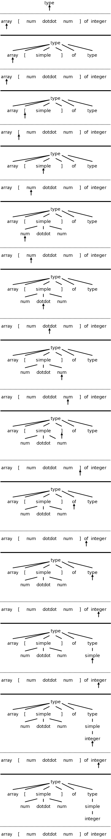
type → array [ simple ] of type
simple → integer
simple → char
simple → num dotdot num
Parsing is easy in principle and for certain grammars (e.g., the two above) it actually is easy. The two fundamental steps (we start at the root since this is top-down parsing) are
When programmed this becomes a procedure for each nonterminal that chooses a production for the node and calls procedures for each nonterminal in the RHS. Thus it is recursive in nature and descends the parse tree. We call these parsers “recursive descent”.
The big problem is what to do if the current node is the LHS of more than one production. The small problem is what do we mean by the “next” node needing a subtree.
The easiest solution to the big problem would be to assume that there is only one production having a given terminal as LHS. There are two possibilities
    expr → term + term - 9
    term → factor / factor
    factor → digit
    digit → 7
But this is very boring. The only possible sentence
is 7/7+7/7-9
    expr → term + term
    term → factor / factor
    factor → ( expr )
This is even worse; there are no (finite) sentences. Only an
infinite sentence beginning (((((((((.
So this won't work. We need to have multiple productions with the same LHS.
How about trying them all? We could do this! If we get stuck where the current tree cannot match the input we are trying to parse, we would backtrack.
Instead, we will look ahead one token in the input and only choose productions that can yield a result starting with this token. Furthermore, we will (in this section) restrict ourselves to predictive parsing in which there is only production that can yield a result starting with a given token. This solution to the big problem also solves the small problem. Since we are trying to match the next token in the input, we must choose the leftmost (nonterminal) node to give children to.
Let's return to pascal array type grammar and consider the three
productions having type as LHS. Even when I write the short
form
type → simple | ↑ id | array [ simple ] of type
I view it as three productions.
For each production P we wish to consider the set FIRST(P) consisting of those tokens that can appear as the first symbol of a string derived from the RHS of P. We actually define FIRST(RHS) rather than FIRST(P), but I often say “first set of the production” when I should really say “first set of the RHS of the production”.
Definition: Let r be the RHS of a production P. FIRST(r) is the set of tokens that can appear as the first symbol in a string derived from r.
To use predictive parsing, we make the following
Assumption: Let P and Q be two productions with the same LHS. Then FIRST(P) and FIRST(Q) are disjoint. Thus, if we know both the LHS and the token that must be first, there is (at most) one production we can apply. BINGO!
This table gives the FIRST sets for our pascal array type example.
| Production | FIRST |
|---|---|
| type → simple | { integer, char, num } |
| type → ↑ id | { ↑ } |
| type → array [ simple ] of type | { array } |
| simple → integer | { integer } |
| simple → char | { char } |
| simple → num dotdot num | { num } |
The three productions with type as LHS have disjoint FIRST sets. Similarly the three productions with simple as LHS have disjoint FIRST sets. Thus predictive parsing can be used. We process the input left to right and call the current token lookahead since it is how far we are looking ahead in the input to determine the production to use. The movie on the right shows the process in action.
Homework:
A. Construct the corresponding table for
  rest → + term rest | - term rest | term
  term → 1 | 2 | 3
B. Can predictive parsing be used?
End of Homework:.
Not all grammars are as friendly as the last example. The first complication is when ε occurs in a RHS. If this happens or if the RHS can generate ε, then ε is included in FIRST.
But ε would always match the current input position!
The rule is that if lookahead is not in FIRST of any production with the desired LHS, we use the (unique!) production (with that LHS) that has ε as RHS.
The second edition, which I just obtained now does a C instead of a pascal example. The productions are
stmt → expr ;
| if ( expr ) stmt
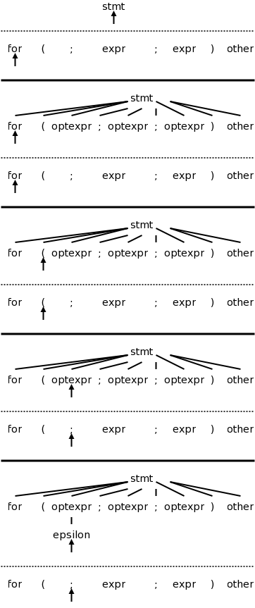
| for ( optexpr ; optexpr ; optexpr ) stmt
| other
optexpr → expr | ε
For completeness, on the right is the beginning of a movie for the C example. Note the use of the ε-production at the end since no other entry in FIRST will match ;
Predictive parsers are fairly easy to construct as we will now see. Since they are recursive descent parsers we go top-down with one procedure for each nonterminal. Do remember that we must have disjoint FIRST sets for all the productions having a given nonterminal as LHS.
The book has code at this point. We will see code later in this chapter.
Another complication. Consider
expr → expr + term
expr → term
For the first production the RHS begins with the LHS. This is called left recursion. If a recursive descent parser would pick this production, the result would be that the next node to consider is again expr and the lookahead has not changed. An infinite loop occurs.
Consider instead
expr → term rest
rest → + term rest
rest → ε
Both pairs of productions generate the same possible token strings,
namely
term + term + ... + term
The second pair is called right recursive since the RHS ends (has on
the right) the LHS.
If you draw the parse trees generated, you will see
that, for left recursive productions, the tree grows to the left; whereas,
for right recursive, it grows to the right.
Note also that, according to the trees generated by the first pair,
the additions are performed right to left; whereas, for the second
pair, they are performed left to right.
That is, for
term + term + term
the tree from the first pair has the left + at the top (why?);
whereas, the tree from the second pair has the right + at the top.
In general, for any A, R, α, and β, we can replace the pair
A → A α | β
with the triple
A → β R
R → α R | ε
For the example above A is “expr”, R is “rest”, α is “+ term”, and β is “term”.
Objective: an infix to postfix translator for expressions. We start with just plus and minus, specifically the expressions generated by the following grammar. We include a set of semantic actions with the grammar. Note that finding a grammar for the desired language is one problem, constructing a translator for the language given a grammar is another problem. We are tackling the second problem.
  expr → expr + term { print('+') }
  expr → expr - term { print('-') }
  expr → term
  term → 0           { print('0') }
  . . .
  term → 9           { print('9') }
One problem that we must solve is that this grammar is left recursive.
We prefer not to have superfluous nonterminals as they make the parsing less efficient. That is why we don't say that a term produces a digit and a digit produces each of 0,...,9. Ideally the syntax tree would just have the operators + and - and the 10 digits 0,1,...,9. That would be called the abstract syntax tree. A parse tree coming from a grammar is technically called a concrete syntax tree.
We eliminate the left recursion as we did in 2.4. This time there
are two operators + and - so we replace the triple
A → A α | A β | γ
with the quadruple
A → γ R
R → α R | β R | ε
This time we have actions so, for example
α is + term { print('+') }
However, the formulas still hold and we get
  expr → term rest
  rest → + term { print('+') } rest
       | - term { print('-') } rest
       | ε
  term → 0           { print('0') }
       . . .
       | 9           { print('9') }
The C code is in the book. Note the else ; in rest(). This corresponds to the epsilon production. As mentioned previously. The epsilon production is only used when all others fail (that is why it is the else arm and not the then or the else if arms).
These are (useful) programming techniques.
In the first edition this is about 40 lines of C code, 12 of which are single { or }. The second edition has equivalent code in java.
Converts a sequence of characters (the source) into a sequence of tokens. A lexeme is the sequence of characters comprising a single token.
These do not become tokens so that the parser need not worry about them.
The 2nd edition moves the discussion about
x<y versus x<=y
into this new section.
I have left it 2 sections ahead to more closely agree with our
(first edition).
This chapter considers only numerical integer constants. They are computed one digit at a time by value=10*value+digit. The parser will therefore receive the token num rather than a sequence of digits. Recall that our previous parsers considered only one digit numbers.
The value of the constant is stored as the attribute of the token num. Indeed <token,attribute> pairs are passed from the scanner to the parser.
The C statement
sum = sum + x;
contains 4 tokens. The scanner will convert the input into
id = id + id ; (id standing for identifier).
Although there are three id tokens, the first and second represent
the lexeme sum; the third represents x. These must be
distinguished. Many language keywords, for example
“then”, are syntactically the same as identifiers.
These also must be distinguished. The symbol table will accomplish
these tasks.
Care must be taken when one lexeme is a proper subset of another.
Consider
x<y versus x<=y
When the < is read, the scanner needs to read another character
to see if it is an =. But if that second character is y, the
current token is < and the y must be “pushed back”
onto the input stream so that the configuration is the same after
scanning < as it is after scanning <=.
Also consider then versus thenewvalue, one is a keyword and the other an id.
As indicated the scanner reads characters and occasionally pushes one back to the input stream. The “downstream” interface is to the parser to which <token,attribute> pairs are passed.
A few comments on the program given in the text. One inelegance is that, in order to avoid passing a record (struct in C) from the scanner to the parser, the scanner returns the next token and places its attribute in a global variable.
Since the scanner converts digits into num's we can shorten the grammar. Here is the shortened version before the elimination of left recursion. Note that the value attribute of a num is its numerical value.
  expr   → expr + term    { print('+') }
  expr   → expr - term    { print('-') }
  expr   → term
  term   → num            { print(num,value) }
In anticipation of other operators with higher precedence, we
introduce factor and, for good measure, include parentheses for
overriding the precedence. So our grammar becomes.
  expr   → expr + term    { print('+') }
  expr   → expr - term    { print('-') }
  expr   → term
  term   → factor
  factor → ( expr ) | num { print(num,value) }
The factor() procedure follows the familiar recursive descent pattern: find a production with lookahead in FIRST and do what the RHS says.
The symbol table is an important data structure for the entire compiler. For the simple translator, it is primarily used to store and retrieve <lexeme,token> pairs.
insert(s,t) returns the index of a new entry storing the
pair (lexeme s, token t).
lookup(s) returns the index for x or 0 if not there.
Simply insert them into the symbol table prior to examining any input. Then they can be found when used correctly and, since their corresponding token will not be id, any use of them where an identifier is required can be flagged.
insert("div",div)Probably the simplest would be
  struct symtableType {
    char lexeme[BIGNUMBER];
    int  token;
  } symtable[ANOTHERBIGNUMBER];
The space inefficiency of having a fixed size entry for all lexemes is
poor, so the authors use a (standard) technique of concatenating all
the strings into one big string and storing pointers to the beginning
of each of the substrings.
One form of intermediate representation is to assume that the target machine is a simple stack machine (explained very soon). The the front end of the compiler translates the source language into instructions for this stack machine and the back end translates stack machine instructions into instructions for the real target machine.
We use a very simple stack machine
Consider Q := Z; or A[f(x)+B*D] := g(B+C*h(x,y));. (I follow the text and use := for the assignment op, which is written = in C/C++. I am using [] for array reference and () for function call).
From a macroscopic view, we have three tasks.
Note the differences between L-values and R-values
| push v | push v (onto stack) |
|---|---|
| rvalue l | push contents of (location) l |
| lvalue l | push address of l |
| pop | pop |
| := | r-value on tos put into the location specified by l-value 2nd on the stack; both are popped |
| copy | duplicate the top of stack |
Machine instructions to evaluate an expression mimic the postfix form of the expression. That is we generate code to evaluate the left operand, then code to evaluate the write operand, and finally the code to evaluate the operation itself.
For example y := 7 * xx + 6 * (z + w) becomes
  lvalue y
  push 7
  rvalue xx
  *
  push 6
  rvalue z
  rvalue w
  +
  *
  +
  :=
To say this more formally we define two attributes. For any nonterminal, the attribute t gives its translation and for the terminal id, the attribute lexeme gives its string representation.
Assuming we have already given the semantic rules for expr (i.e., assuming that the annotation expr.t is known to contain the translation for expr) then the semantic rule for the assignment statement is
  stmt → id := expr
      { stmt.t := 'lvalue' || id.lexime || expr.t || := }
There are several ways of specifying conditional and unconditional jumps. We choose the following 5 instructions. The simplifying assumption is that the abstract machine supports “symbolic” labels. The back end of the compiler would have to translate this into machine instructions for the actual computer, e.g. absolute or relative jumps (jump 3450 or jump +500).
| label l | target of jump |
|---|---|
| goto l | |
| gofalse | pop stack; jump if value is false |
| gotrue | pop stack; jump if value is true |
| halt |
Fairly simple. Generate a new label using the assumed function newlabel(), which we sometimes write without the (), and use it. The semantic rule for an if statement is simply
  stmt → if expr then stmt1 { out := newlabel();
                           stmt.t := expr.t || 'gofalse' out || stmt1.t || 'label' out
Rewriting the above as a semantic action (rather than a rule) we get the following, where emit() is a function that prints its arguments in whatever form is required for the abstract machine (e.g., it deals with line length limits, required whitespace, etc).
  stmt → if
	 expr      { out := newlabel; emit('gofalse', out); }
	 then
         stmt1     { emit('label', out) }
Don't forget that expr is itself a nonterminal. So by the time we reach out:=newlabel, we will have already parsed expr and thus will have done any associated actions, such as emit()'ing instructions. These instructions will have left a boolean on the tos. It is this boolean that is tested by the emitted gofalse.
More precisely, the action written to the right of expr will be the third child of stmt in the tree. Since a postorder traversal visits the children in order, the second child “expr” will have been visited (just) prior to visiting the action.
Look how simple it is! Don't forget that the FIRST sets for the productions having stmt as LHS are disjoint!
  procedure stmt
    integer test, out;
    if lookahead = id then       // first set is {id} for assignment
      emit('lvalue', tokenval);  // pushes lvalue of lhs
      match(id);                 // move past the lhs]
      match(':=');               // move past the :=
      expr;                      // pushes rvalue of rhs on tos
      emit(':=');                // do the assignment (Omitted in book)
    else if lookahead = 'if' then
      match('if');               // move past the if
      expr;                      // pushes boolean on tos
      out := newlabel();
      emit('gofalse', out);      // out is integer, emit makes a legal label
      match('then');             // move past the then
      stmt;                      // recursive call
      emit('label', out)         // emit again makes out legal
    else if ...                  // while, repeat/do, etc
    else error();
  end stmt;
Full code for a simple infix to postfix translator. This uses the concepts developed in 2.5-2.7 (it does not use the abstract stack machine material from 2.8). Note that the intermediate language we produced in 2.5-2.7, i.e., the attribute .t or the result of the semantic actions, is essentially the final output desired. Hence we just need the front end.
The grammar with semantic actions is as follows. All the actions come at the end since we are generating postfix. this is not always the case.
   start → list eof
    list → expr ; list
    list →  ε                   // would normally use | as below
    expr → expr + term      { print('+') }
         | expr - term      { print('-'); }
         | term
    term → term * factor    { print('*') }
         | term / factor    { print('/') }
         | term div factor  { print('DIV') }
         | term mod factor  { print('MOD') }
         | factor
  factor → ( expr )
         | id               { print(id.lexeme) }
         | num              { print(num.value) }
Eliminate left recursion to get
        start → list eof
	 list → expr ; list
	      | ε
	 expr → term moreterms
    moreterms → + term { print('+') } moreterms
	      | - term { print('-') } moreterms
	      | ε
         term | factor morefactors
  morefactors → * factor { print('*') } morefactors
	      | / factor { print('/') } morefactors
	      | div factor { print('DIV') } morefactors
	      | mod factor { print('MOD') } morefactors
	      | ε
       factor → ( expr )
              | id               { print(id.lexeme) }
              | num              { print(num.value) }
Show “A+B;” on board starting with “start”.
Contains lexan(), the lexical analyzer, which is called by the parser to obtain the next token. The attribute value is assigned to tokenval and white space is stripped.
| lexme | token | attribute value |
|---|---|---|
| white space | ||
| sequence of digits | NUM | numeric value |
| div | DIV | |
| mod | MOD | |
| other seq of a letter then letters and digits | ID | index into symbol table |
| eof char | DONE | |
| other char | that char | NONE |
Using a recursive descent technique, one writes routines for each nonterminal in the grammar. In fact the book combines term and morefactors into one routine.
  term() {
    int t;
    factor();
    // now we should call morefactorsl(), but instead code it inline
    while(true)              // morefactor nonterminal is right recursive
       switch (lookahead) {  // lookahead set by match()
       case '*': case '/': case DIV: case MOD: // all the same
          t = lookahead;     // needed for emit() below
          match(lookahead)   // skip over the operator
          factor();          // see grammar for morefactors
          emit(t,NONE);
          continue;          // C semantics for case
       default:              // the epsilon production
          return;
Other nonterminals similar.
The routine emit().
The insert(s,t) and lookup(s) routines described previously are in symbol.c The routine init() preloads the symbol table with the defined keywords.
Does almost nothing. The only help is that the line number, calculated by lexan() is printed.
One reason is that much was deliberately simplified. Specifically note that
Also, I presented the material way too fast to expect full understanding.
Homework: Read chapter 3.
Two methods to construct a scanner (lexical analyzer).
Note that the speed (of the lexer not of the code generated by the compiler) and error reporting/correction are typically much better for a handwritten lexer. As a result most production-level compiler projects write their own lexers
The lexer is called by the parser when the latter is ready to process another token.
The lexer also might do some housekeeping such as eliminating whitespace and comments. Some call these tasks scanning, but others call the entire task scanning.
After the lexer, individual characters are no longer examined by the compiler; instead tokens (the output of the lexer) are used.
Why separate lexical analysis from parsing? The reasons are basically software engineering concerns.
Note the circularity of the definitions for lexeme and pattern.
Common token classes.
Homework: 3.3.
We saw an example of attributes in the last chapter.
For tokens corresponding to keywords, attributes are not needed since the name of the token tells everything. But consider the token corresponding to integer constants. Just knowing that the we have a constant is not enough, subsequent stages of the compiler need to know the value of the constant. Similarly for the token identifier we need to distinguish one identifier from another. The normal method is for the attribute to specify the symbol table entry for this identifier.
We saw in this movie an example where parsing got “stuck” because we reduced the wrong part of the input string. We also learned about FIRST sets that enabled us to determine which production to apply when we are operating left to right on the input. For predictive parsers the FIRST sets for a given nonterminal are disjoint and so we know which production to apply. In general the FIRST sets might not be disjoint so we have to try all the productions whose FIRST set contains the lookahead symbol.
All the above assumed that the input was error free, i.e. that the source was a sentence in the language. What should we do when the input is erroneous and we get to a point where no production can be applied?
The simplest solution is to abort the compilation stating that the program is wrong, perhaps giving the line number and location where the parser could not proceed.
We would like to do better and at least find other errors. We could perhaps skip input up to a point where we can begin anew (e.g. after a statement ending semicolon), or perhaps make a small change to the input around lookahead so that we can proceed.