================ Start Lecture #1 ================
I start at Chapter 0 so that when we get to chapter 1, the numbering will agree with the text.
There is a web site for the course. You can find it from my home page listed above.
The course text is Aho, Seithi, and Ullman: Compilers: Principles, Techniques, and Tools
Your grade will be a function of your final exam and laboratory assignments (see below). I am not yet sure of the exact weightings for each lab and the final, but will let you know soon.
I use the upper left board for lab/homework assignments and announcements. I should never erase that board. If you see me start to erase an announcement, please let me know.
I try very hard to remember to write all announcements on the upper left board and I am normally successful. If, during class, you see that I have forgotten to record something, please let me know. HOWEVER, if I forgot and no one reminds me, the assignment has still been given.
I make a distinction between homeworks and labs.
Labs are
Homeworks are
Homeworks are numbered by the class in which they are assigned. So any homework given today is homework #1. Even if I do not give homework today, the homework assigned next class will be homework #2. Unless I explicitly state otherwise, all homeworks assignments can be found in the class notes. So the homework present in the notes for lecture #n is homework #n (even if I inadvertently forgot to write it to the upper left board).
You may solve lab assignments on any system you wish, but ...
Good methods for obtaining help include
You may write your lab in Java, C, or C++. Other languages may be possible, but please ask in advance. I need to ensure that the TA is comfortable with the language.
The rules for incompletes and grade changes are set by the school and not the department or individual faculty member. The rules set by GSAS state:
The assignment of the grade Incomplete Pass(IP) or Incomplete Fail(IF) is at the discretion of the instructor. If an incomplete grade is not changed to a permanent grade by the instructor within one year of the beginning of the course, Incomplete Pass(IP) lapses to No Credit(N), and Incomplete Fail(IF) lapses to Failure(F).
Permanent grades may not be changed unless the original grade resulted from a clerical error.
I do not assume you have had a compiler course as an undergraduate, and I do not assume you have had experience developing/maintaining a compiler.
If you have already had a compiler class, this course is probably not appropriate. For example, if you can explain the following concepts/terms, the course is probably too elementary for you.
I do assume you are an experienced programmer. There will be non-trivial programming assignments during this course. Indeed, you will write a compiler for a simple programming language.
I also assume that you have at least a passing familiarity with assembler language. In particular, your compiler will produce assembler language. We will not, however, write significant assembly-language programs.
Our policy on academic integrity, which applies to all graduate courses in the department, can be found here.
Homework Read chapter 1.
A Compiler is a translator from one language, the input or source language, to another language, the output or target language.
Often, but not always, the target language is an assembler language or the machine language for a computer processor.
Modern compilers contain two (large) parts, each of which is often subdivided. These two parts are the front end and the back end.
The front end analyzes the source program, determines its constituent parts, and constructs an intermediate representation of the program. Typically the front end is independent of the target language.
The back end synthesizes the target program from the intermediate representation produced by the front end. Typically the back end is independent of the source language.
This front/back division very much reduces the work for a compiling
system that can handle several (N) source languages and several (M)
target languages. Instead of NM compilers, we need N front ends and
M back ends. For gcc (originally standing for Gnu C Compiler, but
now standing for Gnu Compiler Collection), N=7 and M~30 so the
savings is considerable.
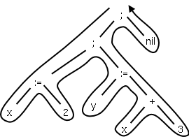
Often the intermediate form produced by the front end is
a syntax tree. In simple cases, such as that shown to the
right corresponding to the C statement sequence
x := 2; y := x + 3;
this tree has constants and
variables (and nil) for leaves and operators for internal nodes.
The back end traverses the tree in “Euler-tour” order and
generates code for each node. (This is quite oversimplified.)
Other “compiler like” applications also use analysis and synthesis. Some examples include
[preprocessor] --> [compiler] --> [assembler] --> [linker] --> [loader]
We will be primarily focused on the second element of the chain, the compiler. Our target language will be assembly language.
Preprocessors are normally fairly simple as in the C language, providing primarily the ability to include files and expand macros. There are exceptions, however. IBM's PL/I, another Algol-like language had quite an extensive preprocessor, which made available at preprocessor time, much of the PL/I language itself (e.g., loops and I believe procedure calls).
Some preprocessors essentially augment the base language, to add additional capabilities. One could consider them as compilers in their own right having as source this augmented language (say fortran augmented with statements for multiprocessor execution in the guise of fortran comments) and as target the original base language (in this case fortran). Often the “preprocessor” inserts procedure calls to implement the extensions at runtime.
Assembly code is an mnemonic version of machine code in which names, rather than binary values, are used for machine instructions, and memory addresses.
Some processors have fairly regular operations and as a result assembly code for them can be fairly natural and not-too-hard to understand. Other processors, in particular Intel's x86 line, have let us charitably say more “interesting” instructions with certain registers used for certain things.
My laptop has one of these latter processors (pentium 4) so my gcc compiler produces code that from a pedagogical viewpoint is less than ideal. If you have a mac with a ppc processor (newest macs are x86), your assembly language is cleaner. NYU's ACF features sun computers with sparc processors, which also have regular instruction sets.
No matter what the assembly language is, an assembler needs to assign memory locations to symbols (called identifiers) and use the numeric location address in the target machine language produced. Of course the same address must be used for all occurrences of a given identifier and two different identifiers must (normally) be assigned two different locations.
The conceptually simplest way to accomplish this is to make two passes over the input (read it once, then read it again from the beginning). During the first pass, each time a new identifier is encountered, an address is assigned and the pair (identifier, address) is stored in a symbol table. During the second pass, whenever an identifier is encountered, its address is looked up in the symbol table and this value is used in the generated machine instruction.
Consider the following trivial C program that computes and returns the xor of the characters in a string.
    int xor (char s[])		// native C speakers say char *s
    {
	int ans = 0;
	int i = 0;

	while (s[i] != 0) {
	    ans = ans ^ s[i];
	    i = i + 1;
	}

	return ans;
    }
The corresponding assembly language program (produced by gcc -S -fomit-frame-pointer) is
	.file	"xor.c"
	.text
.globl xor
	.type	xor, @function
xor:
	subl	$8, %esp
	movl	$0, 4(%esp)
	movl	$0, (%esp)
.L2:
	movl	(%esp), %eax
	addl	12(%esp), %eax
	cmpb	$0, (%eax)
	je	.L3
	movl	(%esp), %eax
	addl	12(%esp), %eax
	movsbl	(%eax),%edx
	leal	4(%esp), %eax
	xorl	%edx, (%eax)
	movl	%esp, %eax
	incl	(%eax)
	jmp	.L2
.L3:
	movl	4(%esp), %eax
	addl	$8, %esp
	ret
	.size	xor, .-xor
	.section	.note.GNU-stack,"",@progbits
	.ident	"GCC: (GNU) 3.4.6 (Gentoo 3.4.6-r1, ssp-3.4.5-1.0, pie-8.7.9)"
You should be able to follow everything from xor: to ret. Indeed most of the rest can be omitted (.globl g is needed). That is the following assembly program gives the same results.
.globl xor
xor:
	subl	$8, %esp
	movl	$0, 4(%esp)
	movl	$0, (%esp)
.L2:
	movl	(%esp), %eax
	addl	12(%esp), %eax
	cmpb	$0, (%eax)
	je	.L3
	movl	(%esp), %eax
	addl	12(%esp), %eax
	movsbl	(%eax),%edx
	leal	4(%esp), %eax
	xorl	%edx, (%eax)
	movl	%esp, %eax
	incl	(%eax)
	jmp	.L2
.L3:
	movl	4(%esp), %eax
	addl	$8, %esp
	ret
What is happening in this program?
Lab assignment 1 is available on the class web site. The programming is trivial; you are just doing inclusive (i.e., normal) OR rather than XOR I just did. The point of the lab is to give you a chance to become familiar with your compiler and assembler.
Linkers, a.k.a. linkage editors combine the output of the assembler for several different compilations. That is the horizontal line of the diagram above should really be a collection of lines converging on the linker. The linker has another input, namely libraries, but to the linker the libraries look like other programs compiled and assembled. The two primary tasks of the linker are
The assembler processes one file at a time. Thus the symbol table produced while processing file A is independent of the symbols defined in file B, and conversely. Thus, it is likely that the same address will be used for different symbols in each program. The technical term is that the (local) addresses in the symbol table for file A are relative to file A; they must be relocated by the linker. This is accomplished by adding the starting address of file A (which in turn is the sum of the lengths of all the files processed previously in this run) to the relative address.
Assume procedure f, in file A, and procedure g, in file B, are compiled (and assembled) separately. Assume also that f invokes g. Since the compiler and assembler do not see g when processing f, it appears impossible for procedure f to know where in memory to find g.
The solution is for the compiler to indicated in the output of the file A compilation that the address of g is needed. This is called a use of g When processing file B, the compiler outputs the (relative) address of g. This is called the definition of g. The assembler passes this information to the linker.
The simplest linker technique is to again make two passes. During the first pass, the linker records in its “external symbol table” (a table of external symbols, not a symbol table that is stored externally) all the definitions encountered. During the second pass, every use can be resolved by access to the table.
I will be covering the linker in more detail tomorrow at 5pm in 2250, OS Design
After the linker has done its work, the resulting “executable file” can be loaded by the operating system into central memory. The details are OS dependent. With early single-user operating systems all programs would be loaded into a fixed address (say 0) and the loader simply copies the file to memory. Today it is much more complicated since (parts of) many programs reside in memory at the same time. Hence the compiler/assembler/linker cannot know the real location for an identifier. Indeed, this real location can change.
More information is given in any OS course (e.g., 2250 given wednesdays at 5pm).
Conceptually, there are three phases of analysis with the output of one phase the input of the next. The phases are called lexical analysis or scanning, syntax analysis or parsing, and semantic analysis.
The character stream input is grouped into tokens. For example, any one of the following
  x3 := y + 3;
  x3  :=   y   +   3   ;
  x3   :=y+ 3  ;
but not
x 3 := y + 3;would be grouped into
Note that non-significant blanks are normally removed during scanning. In C, most blanks are non-significant. Blanks inside strings are an exception.
Note that we could define identifiers, numbers, and the various
symbols and punctuation can be defined without recursion (compare
with parsing below).
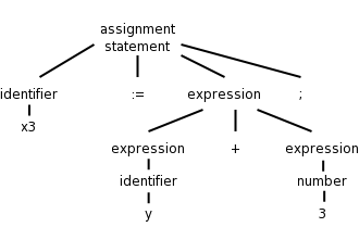
Parsing involves a further grouping in which tokens are grouped into grammatical phrases, which are normally represented in a parse tree. For example
x3 := y + 3;would be parsed into the tree on the right.
This parsing would result from a grammar containing rules such as
  asst-stmt --> id := expr ;
  expr --> number
        |  id
        |  expr + expr
Note the recursive definition of expression (expr). Note also the hierarchical decomposition in the figure on the right.
The division between scanning and parsing is somewhat arbitrary,
but invariably if a recursive definition is involved, it is
considered parsing not scanning.
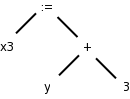
Often we utilize a simpler tree called the syntax tree with operators as interior nodes and operands as the children of the operator. The syntax tree on the right corresponds to the parse tree above it.
(Technical point.) The syntax tree represents an assignment expression not an assignment statement. In C an assignment statement includes the trailing semicolon. That is, in C (unlike in Algol) the semicolon is a statement terminator not a statement separator.
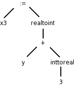
There is more to a front end than simply syntax. The compiler needs semantic information, e.g., the types (integer, real, pointer to array of integers, etc) of the objects involved. This enables checking for semantic errors and inserting type conversion where necessary.
For example, if y was declared to be a real and x3 an integer, We need to insert (unary, i.e., one operand) conversion operators “inttoreal” and “realtoint” as shown on the right.
Illustrates the use of hierarchical grouping for formatting languages (Tex and EQN are used as examples). For example shows how you can get subscripted superscripts (or superscripted subscripts)
[scanner]→[parser]→[sem anal]→[inter code gen]→[opt1]→[code gen]→[opt2]
We just examined the first three phases. Modern, high-performance
compilers, are dominated by their extensive optimization
phases, which occur before, during, and after code generation. Note
that optimization is most assuredly an inaccurate, albeit standard,
terminology, as the resulting code is not optimal.
As we have seen when discussing assemblers and linkers, a symbol table is used to maintain information about symbols. The compiler uses a symbol to maintain information across phases as well as within each phase. One key item stored with each symbol is the corresponding type, which is determined during semantic and used (among other places) during code generation.
As you have doubtless noticed, not all programming efforts produce correct programs. If the input to the compiler is not a legal source language program, errors must be detected and reported. It is often much easier to detect that the program is not legal (e.g., the parser reaches a point where the next token cannot legally occur) than to deduce what is the actual error (which may have occurred earlier). It is even harder to reliably deduce what the intended correct program should be.
The scanner converts
x3 := y + 3;into
id1 := id2 + 3 ;where id is short for identifier.
This is processed by the parser and semantic analyzer to produce the two trees shown above here and here. On some systems, the tree would not contain the symbols themselves as shown in the figures. Instead the tree would contain leaves of the form idi which in turn would refer to the corresponding entries in the symbol table.
Many compilers first generate code for an “idealized machine”. For example, the intermediate code generated would assume that the target has an unlimited number of registers and that any register can be used for any operation. Another common assumption is that all machine operations take three operands, two source and one target.
With these assumptions one generates “three-address code” by walking the semantic tree. Our example C instruction would produce
temp1 := inttoreal(3)
temp2 := id2 + temp1
temp3 := realtoint(temp2)
id1 := temp3
We see that three-address code can include instructions with fewer than 3 operands.
Sometimes three-address code is called quadruples because one can view the previous code sequence as
inttoreal temp1 3     --
add       temp2 id2   temp1
realtoint temp3 temp2 --
assign    id1   temp3 --
Each “quad” has the form
operation target source1 source2
This is a very serious subject, one that we will not really do justice to in this introductory course. Some optimizations are fairly easy to see.
add temp2 id2 3.0
realtoint id1 temp2
Modern processors have only a limited number of register. Although some processors, such as the x86, can perform operations directly on memory locations, we will for now assume only register operations. Some processors (e.g., the MIPS architecture) use three-address instructions. However, some processors permit only two addresses; the result overwrites the second source. With these assumptions, code something like the following would be produced for our example, after first assigning memory locations to id1 and id2.
MOVE id2,  R1
ADD  #3.0, R1
RTOI R1,   R2
MOVE R2,   id1
I found it more logical to treat these topics (preprocessors, assemblers, linkers, and loaders) earlier.
Logically each phase is viewed as a separate program that reads input and produces output for the next phase, i.e., a pipeline. In practice some phases are combined.
We discussed this previously.
Aho, Sethi, Ullman assert only limited success in producing several compilers for a single machine using a common back end. That is a rather pessimistic view and I wonder if the 2nd edition will change in this area.
The term pass is used to indicate that the entire input is read during this activity. So two passes, means that the input is read twice. We have discussed two pass approaches for both assemblers and linkers. If we implement each phase separately and use multiple phases for some of them, the compiler will perform a large number of I/O operations, an expensive undertaking.
As a result techniques have been developed to reduce the number of passes. We will see in the next chapter how to combine the scanner, parser, and semantic analyzer into one phase. Consider the parser. When it needs another token, rather than reading the input file (presumably produced by the scanner), the parser calls the scanner instead. At selected points during the production of the syntax tree, the parser calls the “code generator”, which performs semantic analysis as well as generating a portion of the intermediate code.
One problem with combining phases, or with implementing a single phase in one pass, is that it appears that an internal form of the entire program will need to be stored in memory. This problem arises because the downstream phase may need early in its execution information that the upstream phase produces only late in its execution. This motivated the use of symbol tables and a two pass approach. However, a clever one-pass approach is often possible.
Consider the assembler (or linker). The good case is when the definition precedes all uses so that the symbol table contains the value of the symbol prior to that value being needed. Now consider the harder case of one or more uses preceding the definition. When a not yet defined symbol is first used, an entry is placed in the symbol table, pointing to this use and indicating that the definition has not yet appeared. Further uses of the same symbol attach their addresses to a linked list of “undefined uses” of this symbol. When the definition is finally seen, the value is placed in the symbol table, and the linked list is traversed inserting the value in all previously encountered uses. Subsequent uses of the symbol will find its definition in the table.
This technique is called backpatching.
Originally, compilers were written “from scratch”, but now the situation is quite different. A number of tools are available to ease the burden.
We will study tools that generate scanners and parsers. This will involve us in some theory, regular expressions for scanners and various grammars for parsers. These techniques are fairly successful. One drawback can be that they do not execute as fast as “hand-crafted” scanners and parsers.
We will also see tools for syntax-directed translation and automatic code generation. The automation in these cases is not as complete.
Finally, there is the large area of optimization. This is not automated; however, a basic component of optimization is “data-flow analysis” (how are values transmitted between parts of a program) and there are tools to help with this task.
Homework: Read chapter 2.
Implement a very simple compiler.
The source language is infix expressions consisting of digits, +,
and -; the target is postfix expressions with the same components.
The compiler will convert
7+4-5 to 74+5-.
Actually, our simple compiler will handle a few other operators as well.
We will tokenize
the input (i.e., write a scanner), model
the syntax of the source, and let this syntax direct the translation.
This will be “done right” in the next two chapters.
A context-free grammar (CFG) consists of
Example:
  Terminals: 0 1 2 3 4 5 6 7 8 9 + -
  Nonterminals: list digit
  Productions: list → list + digit
               list → list - digit
               list → digit
               digit → 0 | 1 | 2 | 3 | 4 | 5 | 6 | 7 | 8 | 9
  Start symbol: list
Watch how we can generate the input 7+4-5 starting with the start symbol, applying productions, and stopping when no productions are possible (we have only terminals).
  list → list - digit
       → list - 5
       → list + digit - 5
       → list + 4 - 5
       → digit + 4 - 5
       → 7 + 4 - 5
Homework: 2.1a, 2.1c, 2.2a-c (don't worry about “justifying” your answers).
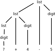
The compiler front end runs the above procedure in reverse! It starts with the string 7+4-5 and gets back to list (the “start” symbol). Reaching the start symbol means that the string is in the language generated by the grammar. While running the procedure in reverse, the front end builds up the parse tree on the right.
You can read off the productions from the tree. For any internal (i.e.,non-leaf) tree node, its children give the right hand side (RHS) of a production having the node itself as the LHS.
The leaves of the tree, read from left to right, is called the yield of the tree. We call the tree a derivation of its yield from its root. The tree on the right is a derivation of 7+4-5 from list.
Homework: 2.1b
An ambiguous grammar is one in which there are two or more parse trees yielding the same final string. We wish to avoid such grammars.
The grammar above is not ambiguous. For example 1+2+3 can be parsed only one way; the arithmetic must be done left to right. Note that I am not giving a rule of arithmetic, just of this grammar. If you reduced 2+3 to list you would be stuck since it is impossible to generate 1+list.
Homework: 2.3 (applied only to parts a, b, and c of 2.2)
Our grammar gives left associativity. That is, if you traverse the
tree in postorder and perform the indicated arithmetic you will
evaluate the string left to right. Thus 8-8-8 would evaluate to
-8. If you wished to generate right associativity (normally
exponentiation is right associative, so 2**3**2 gives 512 not 64),
you would change the first two productions to
list → digit + list and list → digit - list
We normally want * to have higher precedence than +. We do this by using an additional nonterminal to indicate the items that have been multiplied. The example below gives the four basic arithmetic operations their normal precedence unless overridden by parentheses. Redundant parentheses are permitted. Equal precedence operations are performed left to right.
expr   → expr + term | expr - term | term
term   → term * factor | term / factor | factor
factor → digit | ( expr )
digit  → 0 | 1 | 2 | 3 | 4 | 5 | 6 | 7 | 8 | 9
We use | to indicate that a nonterminal has multiple possible right hand side. So
A → B | Cis simply shorthand for
  A → B
  A → C
Do the examples 1+2/3-4*5 and (1+2)/3-4*5 on the board.
Note how the precedence is enforced by the grammar; slick!
Keywords are very helpful for distinguishing statements from one another.
stmt → id := expr
     | if expr then stmt
     | if expr then stmt else stmt
     | while expr do stmt
     | begin opt-stmts end
opt-stmts → stmt-list | ε
stmt-list → stmt-list ; stmt | stmt
Remark:
Homework: 2.16a, 2.16b
Specifying the translation of a source language construct in terms of attributes of its syntactic components.
Operator after operand. Parentheses are not needed. The normal notation we used is called infix. If you start with an infix expression, the following algorithm will give you the equivalent postfix expression.
One question is, given say 1+2-3, what is E, F and op? Does E=1+2, F=3, and op=+? Or does E=1, F=2-3 and op=+? This is the issue of precedence mentioned above. To simplify the present discussion we will start with fully parenthesized infix expressions.
Example: 1+2/3-4*5
Example: Now do (1+2)/3-4*5
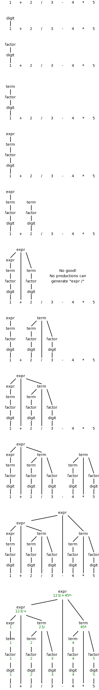
We want to “decorate” the parse trees we construct with “annotations” that give the value of certain attributes of the corresponding node of the tree. We will do the example of translating infix to postfix with 1+2/3-4*5. We use the following grammar, which follows the normal arithmetic terminology where one multiplies and divides factors to obtain terms, which in turn are added and subtracted to form expressions.
  expr   → expr + term | expr - term | term
  term   → term * factor | term / factor | factor
  factor → digit | ( expr )
  digit  → 0 | 1 | 2 | 3 | 4 | 5 | 6 | 7 | 8 | 9
This grammar supports parentheses, although our example does not use them. On the right is a “movie” in which the parse tree is build from this example.
The attribute we will associate with the nodes is the text to be used to print the postfix form of the string in the leaves below the node. In particular the value of this attribute at the root is the postfix form of the entire source.
The book does a simpler grammar (no *, /, or parentheses) for a simpler example. You might find that one easier. The book also does another grammar describing commands to give a robot to move north, east, south, or west by one unit at a time. The attributes associated with the nodes are the current position (for some nodes, including the root) and the change in position caused by the current command (for other nodes).
Definition: A syntax-directed definition is a grammar together with a set of “semantic rules” for computing the attribute values. A parse tree augmented with the attribute values at each node is called an annotated parse tree.
For the bottom-up approach I will illustrate now, we annotate a node after having annotated its children. Thus the attribute values at a node can depend on the children of the node but not the parent of the node. We call these synthesized attributes, since they are formed by synthesizing the attributes of the children.
In chapter 5, when we study top-down annotations as well, we will introduce “inherited” attributes that are passed down from parents to children.
We specify how to synthesize attributes by giving the semantic rules together with the grammar. That is we give the syntax directed definition.
| Production | Semantic Rule |
|---|---|
| expr → expr1 + term | expr.t := expr1.t || term.t || '+' |
| expr → expr1 - term | expr.t := expr1.t || term.t || '-' |
| expr → term | expr.t := term.t |
| term → term1 * factor | term.t := term1.t || factor.t || '*' |
| term → term1 / factor | term.t := term1.t || factor.t || '/' |
| term → factor | term.t := factor.t |
| factor → digit | factor.t := digit.t |
| factor → ( expr ) | factor.t := expr.t |
| digit → 0 | digit.t := '0' |
| digit → 1 | digit.t := '1' |
| digit → 2 | digit.t := '2' |
| digit → 3 | digit.t := '3' |
| digit → 4 | digit.t := '4' |
| digit → 5 | digit.t := '5 |
| digit → 6 | digit.t := '6' |
| digit → 7 | digit.t := '7' |
| digit → 8 | digit.t := '8' |
| digit → 9 | digit.t := '9' |
We apply these rules bottom-up (starting with the geographically lowest productions, i.e., the lowest lines on the page) and get the annotated graph shown on the right. The annotation are drawn in green.
Homework: Draw the annotated graph for (1+2)/3-4*5.
As mentioned in this chapter we are annotating bottom-up. This corresponds to doing a depth-first traversal of the (unannotated) parse tree to produce the annotations. It is often called a postorder traversal because a parent is visited after (i.e., post) its children are visited.
The bottom-up annotation scheme generates the final result as the annotation of the root. In our infix → postfix example we get the result desired by printing the root annotation. Now we consider another technique that produces its results incrementally.
Instead of giving semantic rules for each production (and thereby generating annotations) we can embed program fragments called semantic actions within the productions themselves.
In diagrams the semantic action is connected to the node with a distinctive, often dotted, line. The placement of the actions determine the order they are performed. Specifically, one executes the actions in the order they are encountered in a postorder traversal of the tree.
Definition: A syntax-directed translation scheme is a context-free grammar with embedded semantic actions.
For our infix → postfix translator, the parent either just
passes on the attribute of its (only) child or concatenates them
left to right and adds something at the end. The equivalent
semantic actions would be either to print the new item or print
nothing.
Here are the semantic actions corresponding to a few of the rows of the table above. Note that the actions are enclosed in {}.
expr → expr + term    { print('+') }
expr → expr - term    { print('-') }
term → term / factor  { print('/') }
term → factor         { null }
digit → 3             { print('3') }
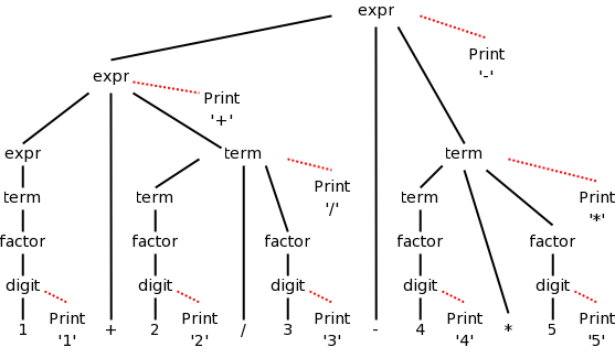
The diagram for 1+2/3-4*5 with attached semantic actions is shown on the right.
Given an input, e.g. our favorite 1+2/3-4*5, we just do a depth first (postorder) traversal of the corresponding diagram and perform the semantic actions as they occur. When these actions are print statements as above, we can be said to be emitting the translation.
Do a depth first traversal of the diagram on the board, performing the semantic actions as they occur, and confirm that the translation emitted is in fact 123/+45*-, the postfix version of 1+2/3-4*5
Homework: Produce the corresponding diagram for (1+2)/3-4*5.
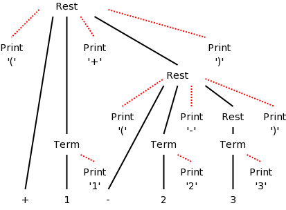
When we produced postfix, all the prints came at the end (so that the children were already “printed”. The { actions } do not need to come at the end. We illustrate this by producing infix arithmetic (ordinary) notation from a prefix source.
In prefix notation the operator comes first so +1-23 evaluates to zero. Consider the following grammar. It translates prefix to infix for the simple language consisting of addition and subtraction of digits between 1 and 3 without parentheses (prefix notation and postfix notation do not use parentheses). The resulting parse tree for +1-23 is shown on the right. Note that the output language (infix notation) has parentheses.
  rest → + term rest | - term rest | term
  term → 1 | 2 | 3
The table below shows the semantic actions or rules needed for our
translator.
| Production with Semantic Action | Semantic Rule |
|---|---|
| rest → { print('(') } + term { print('+') } rest { print(')') } | rest.t := '(' || term.t || '+' || rest.t || ')' |
| rest → { print('(') } - term { print('-') } rest { print(')') } | rest.t := '(' || term.t || '-' || rest.t || ')' |
| rest → term | rest.t := term.t |
| term → 1 { print('1') } | term.t := '1' |
| term → 2 { print('2') } | term.t := '2' |
| term → 3 { print('3') } | term.t := '3' |
Homework: 2.8.
If the semantic rules of a syntax-directed definition all have the property that the new annotation for the left hand side (LHS) of the production is just the concatenation of the annotations for the nonterminals on the RHS in the same order as the nonterminals appear in the production, we call the syntax-directed definition simple. It is still called simple if new strings are interleaved with the original annotations. So the example just done is a simple syntax-directed definition.
Remark: We shall see later that, in many cases a simple syntax-directed definition permits one to execute the semantic actions while parsing and not construct the parse tree at all.