Operating Systems

Note: Should have done this last time Consider three processes all starting at time 0. One requires 1ms, the second 100ms, the third 10sec (seconds). Compute the total/average waiting time for (P)SJF and compare to RR q=1ms, FCFS, and PS.

Remark: Recall that SFJ/PSFJ do a good job of minimizing the average waiting time. The problem with them is the difficulty in finding the job whose next CPU burst is minimal. We now learn two scheduling algorithms that attempt to do this (approximately). The first one does this statically, presumably with some manual help; the second is dynamic and fully automatic.

Multilevel Queues (**, **, MLQ, **)

Put different classes of processs in different queues

• Processs do not move from one queue to another.
• Can have different policies on the different queues.
  For example, might have a background (batch) queue that is FCFS and one or more foreground queues that are RR.
• Must also have a policy among the queues.
  For example, might have two queues, foreground and background, and give the first absolute priority over the second
  • Might apply aging to prevent background starvation.
  • But might not, i.e., no guarantee of service for background processes. View a background process as a “cycle soaker”.
  • Might have 3 queues, foreground, background, cycle soaker.

Multilevel Feedback Queues (FB, MFQ, MLFBQ, MQ)

As with multilevel queues above we have many queues, but now processs move from queue to queue in an attempt to dynamically separate “batch-like” from interactive processs so that we can favor the latter.

• Remember that average waiting time is achieved by SJF, and this is an attempt to determine dynamically those processes that are interactive, which means have a very short cpu burst.
• Run processs from the highest priority nonempty queue in a RR manner.
• When a process uses its full quanta (looks a like batch process), move it to a lower priority queue.
• When a process doesn't use a full quanta (looks like an interactive process), move it to a higher priority queue.
• A long process with frequent (perhaps spurious) I/O will remain in the upper queues.
• Might have the bottom queue FCFS.
• Many variants.
  For example, might let process stay in top queue 1 quantum, next queue 2 quanta, next queue 4 quanta (i.e., sometimes return a process to the rear of the same queue it was in if the quantum expires).

Theoretical Issues

Considerable theory has been developed.

• NP completeness results abound.
• Much work in queuing theory to predict performance.
• Not covered in this course.

Medium-Term Scheduling

In addition to the short-term scheduling we have discussed, we add medium-term scheduling in which decisions are made at a coarser time scale.

• Called memory scheduling by Tanenbaum (part of three level scheduling).
• Suspend (swap out) some process if memory is over-committed.
• Criteria for choosing a victim.
  • How long since previously suspended.
  • How much CPU time used recently.
  • How much memory does it use.
  • External priority (pay more, get swapped out less).
• We will discuss medium term scheduling again when we study memory management.

Long Term Scheduling

• “Job scheduling”. Decide when to start jobs, i.e., do not necessarily start them when submitted.
• Force user to log out and/or block logins if over-committed.
  • CTSS (an early time sharing system at MIT) did this to insure decent interactive response time.
  • Unix does this if out of processes (i.e., out of PTEs).
  • “LEM jobs during the day” (Grumman).
• Called admission scheduling by Tanenbaum (part of three level scheduling).
• Many supercomputer sites.

2.5.4: Scheduling in Real Time Systems

Skipped

2.5.5: Policy versus Mechanism

Skipped.

2.5.6: Thread Scheduling

Skipped.

Research on Processes and Threads

Skipped.

Chapter 3: Deadlocks

A deadlock occurs when every member of a set of processes is waiting for an event that can only be caused by a member of the set.

Often the event waited for is the release of a resource.

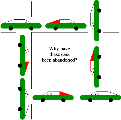
In the automotive world deadlocks are called gridlocks.

• The processes are the cars.
• The resources are the spaces occupied by the cars

Old Reward: I used to give one point extra credit on the final exam for anyone who brings a real (e.g., newspaper) picture of an automotive deadlock. Note that it must really be a gridlock, i.e., motion is not possible without breaking the traffic rules. A huge traffic jam is not sufficient. This was solved last semester so no reward any more. One of the winners in on my office door.

For a computer science example consider two processes A and B that each want to print a file currently on tape.

1. A has obtained ownership of the printer and will release it after printing one file.
2. B has obtained ownership of the tape drive and will release it after reading one file.
3. A tries to get ownership of the tape drive, but is told to wait for B to release it.
4. B tries to get ownership of the printer, but is told to wait for A to release the printer.

Bingo: deadlock!

3.1: Resources

The resource is the object granted to a process.

3.1.1: Preemptable and Nonpreemptable Resources

• Resources come in two types
  1. Preemptable, meaning that the resource can be taken away from its current owner (and given back later). An example is memory.
  2. Non-preemptable, meaning that the resource cannot be taken away. An example is a printer.
• The interesting issues arise with non-preemptable resources so those are the ones we study.
• Life history of a resource is a sequence of
  1. Request
  2. Allocate
  3. Use
  4. Release
• Processes make requests, use the resource, and release the resource. The allocate decisions are made by the system and we will study policies used to make these decisions.

3.1.2: Resource Acquisition

Simple example of the trouble you can get into.

• Two resources and two processes.
• Each process wants both resources.
• Use a semaphore for each. Call them S and T.
• If both processes execute P(S); P(T); --- V(T); V(S)
  all is well.
• But if one executes instead P(T); P(S); -- V(S); V(T)
  disaster! This was the printer/tape example just above.

Recall from the semaphore/critical-section treatment last chapter, that it is easy to cause trouble if a process dies or stays forever inside its critical section; we assume processes do not do this. Similarly, we assume that no process retains a resource forever. It may obtain the resource an unbounded number of times (i.e. it can have a loop forever with a resource request inside), but each time it gets the resource, it must release it eventually.

3.2: Introduction to Deadlocks

To repeat: A deadlock occurs when a every member of a set of processes is waiting for an event that can only be caused by a member of the set.

Often the event waited for is the release of a resource.

3.2.1: (Necessary) Conditions for Deadlock

The following four conditions (Coffman; Havender) are necessary but not sufficient for deadlock. Repeat: They are not sufficient.

1. Mutual exclusion: A resource can be assigned to at most one process at a time (no sharing).
2. Hold and wait: A processing holding a resource is permitted to request another.
3. No preemption: A process must release its resources; they cannot be taken away.
4. Circular wait: There must be a chain of processes such that each member of the chain is waiting for a resource held by the next member of the chain.

The first three are characteristics of the system and resources. That is, for a given system with a fixed set of resources, the first three conditions are either true or false: They don't change with time. The truth or falsehood of the last condition does indeed change with time as the resources are requested/allocated/released.

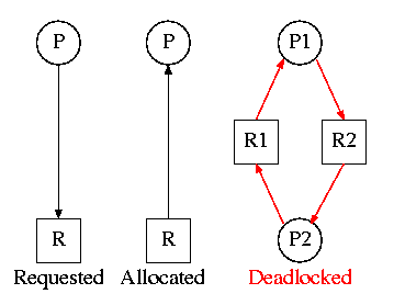
3.2.2: Deadlock Modeling

On the right are several examples of a Resource Allocation Graph, also called a Reusable Resource Graph.

• The processes are circles.
• The resources are squares.
• An arc (directed line) from a process P to a resource R signifies that process P has requested (but not yet been allocated) resource R.
• An arc from a resource R to a process P indicates that process P has been allocated resource R.

Homework: 5.

Consider two concurrent processes P1 and P2 whose programs are.

P1: request R1       P2: request R2
    request R2           request R1
    release R2           release R1
    release R1           release R2

On the board draw the resource allocation graph for various possible executions of the processes, indicating when deadlock occurs and when deadlock is no longer avoidable.

There are four strategies used for dealing with deadlocks.

1. Ignore the problem
2. Detect deadlocks and recover from them
3. Avoid deadlocks by carefully deciding when to allocate resources.
4. Prevent deadlocks by violating one of the 4 necessary conditions.

3.3: Ignoring the problem--The Ostrich Algorithm

The “put your head in the sand approach”.

• If the likelihood of a deadlock is sufficiently small and the cost of avoiding a deadlock is sufficiently high it might be better to ignore the problem. For example if each PC deadlocks once per 100 years, the one reboot may be less painful that the restrictions needed to prevent it.
  
  
• Clearly not a good philosophy for nuclear missile launchers.
  
  
• For embedded systems (e.g., missile launchers) the programs run are fixed in advance so many of the questions Tanenbaum raises (such as many processes wanting to fork at the same time) don't occur.

3.4: Detecting Deadlocks and Recovering From Them

3.4.1: Detecting Deadlocks with Single Unit Resources

Consider the case in which there is only one instance of each resource.

• Thus a request can be satisfied by only one specific resource.
  
  
• In this case the 4 necessary conditions for deadlock are also sufficient.
  
  
• Remember we are making an assumption (single unit resources) that is often invalid. For example, many systems have several printers and a request is given for “a printer” not a specific printer. Similarly, one can have many tape drives.
  
  
• So the problem comes down to finding a directed cycle in the resource allocation graph. Why?
  Answer: Because the other three conditions are either satisfied by the system we are studying or are not in which case deadlock is not a question. That is, conditions 1,2,3 are conditions on the system in general not on what is happening right now.

To find a directed cycle in a directed graph is not hard. The algorithm is in the book. The idea is simple.

1. For each node in the graph do a depth first traversal to see if the graph is a DAG (directed acyclic graph), building a list as you go down the DAG.
   
   
2. If you ever find the same node twice on your list, you have found a directed cycle, the graph is not a DAG, and deadlock exists among the processes in your current list.
   
   
3. If you never find the same node twice, the graph is a DAG and no deadlock occurs.
   
   
4. The searches are finite since the list size is bounded by the number of nodes.