Operating Systems

2.3.4: Sleep and Wakeup

Remark: Tanenbaum does both busy waiting (as above) and blocking (process switching) solutions. We will only do busy waiting, which is easier. Sleep and Wakeup are the simplest blocking primitives. Sleep voluntarily blocks the process and wakeup unblocks a sleeping process. We will not cover these.

Homework: Explain the difference between busy waiting and blocking process synchronization.

2.3.5: Semaphores

Remark: Tannenbaum use the term semaphore only for blocking solutions. I will use the term for our busy waiting solutions. Others call our solutions spin locks.

P and V and Semaphores

The entry code is often called P and the exit code V. Thus the critical section problem is to write P and V so that

loop forever
    P
    critical-section
    V
    non-critical-section

1. Mutual exclusion.
2. No speed assumptions.
3. No blocking by processes in NCS.
4. Forward progress (my weakened version of Tanenbaum's last condition).

Note that I use indenting carefully and hence do not need (and sometimes omit) the braces {} used in languages like C or java.

A binary semaphore abstracts the TAS solution we gave for the critical section problem.

• A binary semaphore S takes on two possible values “open” and “closed”.
• Two operations are supported
• P(S) is

      while (S=closed) {}
      S<--closed     <== This is NOT the body of the while
  

  where finding S=open and setting S<--closed is atomic
• That is, wait until the gate is open, then run through and atomically close the gate
• Said another way, it is not possible for two processes doing P(S) simultaneously to both see S=open (unless a V(S) is also simultaneous with both of them).
• V(S) is simply S<--open

The above code is not real, i.e., it is not an implementation of P. It is, instead, a definition of the effect P is to have.

To repeat: for any number of processes, the critical section problem can be solved by

loop forever
    P(S)
    CS
    V(S)
    NCS

The only specific solution we have seen for an arbitrary number of processes is the one just above with P(S) implemented via test and set.

Remark: Peterson's solution requires each process to know its processor number. The TAS soluton does not. Moreover the definition of P and V does not permit use of the processor number. Thus, strictly speaking Peterson did not provide an implementation of P and V. He did solve the critical section problem.

To solve other coordination problems we want to extend binary semaphores.

• With binary semaphores, two consecutive Vs do not permit two subsequent Ps to succeed (the gate cannot be doubly opened).
• We might want to limit the number of processes in the section to 3 or 4, not always just 1.

Both of the shortcomings can be overcome by not restricting ourselves to a binary variable, but instead define a generalized or counting semaphore.

• A counting semaphore S takes on non-negative integer values
• Two operations are supported
• P(S) is

      while (S=0) {}
      S--
  

  where finding S>0 and decrementing S is atomic
• That is, wait until the gate is open (positive), then run through and atomically close the gate one unit
• Another way to describe this atomicity is to say that it is not possible for the decrement to occur when S=0 and it is also not possible for two processes executing P(S) simultaneously to both see the same necessarily (positive) value of S unless a V(S) is also simultaneous.
• V(S) is simply S++

These counting semaphores can solve what I call the semi-critical-section problem, where you premit up to k processes in the section. When k=1 we have the original critical-section problem.

initially S=k

loop forever
    P(S)
    SCS   <== semi-critical-section
    V(S)
    NCS

Producer-consumer problem

• Two classes of processes
  • Producers, which produce times and insert them into a buffer.
  • Consumers, which remove items and consume them.
• What if the producer encounters a full buffer?
  Answer: It waits for the buffer to become non-full.
• What if the consumer encounters an empty buffer?
  Answer: It waits for the buffer to become non-empty.
• Also called the bounded buffer problem.
  • Another example of active entities being replaced by a data structure when viewed at a lower level (Finkel's level principle).

Initially e=k, f=0 (counting semaphore); b=open (binary semaphore)

Producer                         Consumer

loop forever                     loop forever
    produce-item                     P(f)
    P(e)                             P(b); take item from buf; V(b)
    P(b); add item to buf; V(b)      V(e)
    V(f)                             consume-item

• k is the size of the buffer
• e represents the number of empty buffer slots
• f represents the number of full buffer slots
• We assume the buffer itself is only serially accessible. That is, only one operation at a time.
  • This explains the P(b) V(b) around buffer operations
  • I use ; and put three statements on one line to suggest that a buffer insertion or removal is viewed as one atomic operation.
  • Of course this writing style is only a convention, the enforcement of atomicity is done by the P/V.
• The P(e), V(f) motif is used to force “bounded alternation”. If k=1 it gives strict alternation.

2.3.6: Mutexes

My Terminology

	Busy wait	block/switch
critical	(binary) semaphore	(binary) semaphore
semi-critical	counting semaphore	counting semaphore

Tanenbaum's Terminology

	Busy wait	block/switch
critical	enter/leave region	mutex
semi-critical	no name	semaphore

2.3.7: Monitors

2.3..8: Message Passing

2.4: Classical IPC Problems

2.4.1: The Dining Philosophers Problem

A classical problem from Dijkstra

• 5 philosophers sitting at a round table
• Each has a plate of spaghetti
• There is a fork between each two
• Need two forks to eat

• The obvious solution (pick up right; pick up left) deadlocks.
• Big lock around everything serializes.
• Good code in the book.

The purpose of mentioning the Dining Philosophers problem without giving the solution is to give a feel of what coordination problems are like. The book gives others as well. We are skipping these (again this material would be covered in a sequel course). If you are interested look, for example, here.

Homework: 31 and 32 (these have short answers but are not easy). Note that the problem refers to fig. 2-20, which is incorrect. It should be fig 2-33.

2.4.2: The Readers and Writers Problem

• Two classes of processes.
  • Readers, which can work concurrently.
  • Writers, which need exclusive access.
• Must prevent 2 writers from being concurrent.
• Must prevent a reader and a writer from being concurrent.
• Must permit readers to be concurrent when no writer is active.
• Perhaps want fairness (e.g., freedom from starvation).
• Variants
  1. Writer-priority readers/writers.
  2. Reader-priority readers/writers.

Quite useful in multiprocessor operating systems and database systems. The “easy way out” is to treat all processes as writers in which case the problem reduces to mutual exclusion (P and V). The disadvantage of the easy way out is that you give up reader concurrency. Again for more information see the web page referenced above.

2.4.3: The Sleeping Barber Problem

2.4A: Summary of 2.3 and 2.4

We then defined (binary) Semaphores and showed that a Semaphore easily solves the critical section problem and doesn't require knowledge of how many processes are competing for the critical section. We gave an implementation using Test-and-Set.

We then gave an operational definition of Semaphore (which is not an implementation) and morphed this definition to obtain a Counting (or Generalized) Semaphore, for which we gave NO implementation. I asserted that a counting semaphore can be implemented using 2 binary semaphores and gave a reference.

We defined the Readers/Writers (or Bounded Buffer) Problem and showed that it can be solved using counting semaphores (and binary semaphores, which are a special case).

Finally we briefly discussed some classical problem, but did not give (full) solutions.

2.5: Process Scheduling

Scheduling processes on the processor is often called “process scheduling” or simply “scheduling”.

The objectives of a good scheduling policy include

• Fairness.
• Efficiency.
• Low response time (important for interactive jobs).
• Low turnaround time (important for batch jobs).
• High throughput [the above are from Tanenbaum].
• More “important” processes are favored.
• Interactive processes are favored.
• Repeatability. Dartmouth (DTSS) “wasted cycles” and limited logins for repeatability.
• Fair across projects.
  • “Cheating” in unix by using multiple processes.
  • TOPS-10.
  • Fair share research project.
• Degrade gracefully under load.

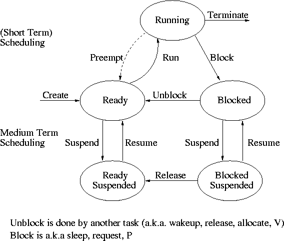
Recall the basic diagram describing process states

For now we are discussing short-term scheduling, i.e., the arcs connecting running <--> ready.

Medium term scheduling is discussed later.

Preemption

It is important to distinguish preemptive from non-preemptive scheduling algorithms.

• Preemption means the operating system moves a process from running to ready without the process requesting it.
• Without preemption, the system implements “run to completion (or yield or block)”.
• The “preempt” arc in the diagram.
• We do not consider yield (a solid arrow from running to ready).
• Preemption needs a clock interrupt (or equivalent).
• Preemption is needed to guarantee fairness.
• Preemption is found in all modern general purpose operating systems.
• Even non preemptive systems can be multiprogrammed (e.g., when processes block for I/O).

Deadline scheduling

This is used for real time systems. The objective of the scheduler is to find a schedule for all the tasks (there are a fixed set of tasks) so that each meets its deadline. The run time of each task is known in advance.

Actually it is more complicated.

• Periodic tasks
• What if we can't schedule all task so that each meets its deadline (i.e., what should be the penalty function)?
• What if the run-time is not constant but has a known probability distribution?

We do not cover deadline scheduling in this course.

The name game

There is an amazing inconsistency in naming the different (short-term) scheduling algorithms. Over the years I have used primarily 4 books: In chronological order they are Finkel, Deitel, Silberschatz, and Tanenbaum. The table just below illustrates the name game for these four books. After the table we discuss each scheduling policy in turn.

Finkel  Deitel  Silbershatz Tanenbaum
-------------------------------------
FCFS    FIFO    FCFS        FCFS
RR      RR      RR          RR
PS      **      PS          PS
SRR     **      SRR         **    not in tanenbaum
SPN     SJF     SJF         SJF
PSPN    SRT     PSJF/SRTF   --    unnamed in tanenbaum
HPRN    HRN     **          **    not in tanenbaum
**      **      MLQ         **    only in silbershatz
FB      MLFQ    MLFQ        MQ

Remark: For an alternate organization of the scheduling algorithms (due to Eric Freudenthal and presented by him Fall 2002) click here.

First Come First Served (FCFS, FIFO, FCFS, --)

If the OS “doesn't” schedule, it still needs to store the list of ready processes in some manner. If it is a queue you get FCFS. If it is a stack (strange), you get LCFS. Perhaps you could get some sort of random policy as well.

• Only FCFS is considered.
• Non-preemptive.
• The simplist scheduling policy.
• In some sense the fairest since it is first come first served. But perhaps that is not so fair--Consider a 1 hour job submitted one second before a 3 second job.
• The most efficient usage of cpu since the scheduler is very fast.

Round Robin (RR, RR, RR, RR)

• An important preemptive policy.
• Essentially the preemptive version of FCFS.
• Note that RR works well if you have a 1 hr job and then a 3 second job.
• The key parameter is the quantum size q.
• When a process is put into the running state a timer is set to q.
• If the timer goes off and the process is still running, the OS preempts the process.
  • This process is moved to the ready state (the preempt arc in the diagram), where it is placed at the rear of the ready list.
  • The process at the front of the ready list is removed from the ready list and run (i.e., moves to state running).
  • Note that the ready list is being treated as a queue. Indeed it is sometimes called the ready queue, but not by me since for other scheduling algorithms it is not accessed in a FIFO manner.
• When a process is created, it is placed at the rear of the ready list.
• As q gets large, RR approaches FCFS. Indeed if q is larger that the longest time a process can run before terminating or blocking, then RR IS FCFS. A good way to see this is to look at my favorite diagram and note the three arcs leaving running. They are “triggered” by three conditions: process terminating, process blocking, and process preempted. If the first condition to trigger is never preemption, we can erase the arc and then RR becomes FCFS.
• As q gets small, RR approaches PS (Processor Sharing, described next)
• What value of q should we choose?
  • Trade-off
  • Small q makes system more responsive, a long compute-bound job cannot starve a short job.
  • Large q makes system more efficient since less process switching.
  • A reasonable time for q is about 1ms (millisecond = 1/1000 second). This means each other job can delay your job by at most 1ms (plus the context switch time CS, which is much less than 1ms). Also the overhead is CS/(CS+q), which is small.

Homework: 26, 35, 38.

Homework: Give an argument favoring a large quantum; give an argument favoring a small quantum.

Process	CPU Time	Creation Time
P1	20	0
P2	3	3
P3	2	5

Homework: (Remind me to discuss this last one in class next time): Consider the set of processes in the table below. When does each process finish if RR scheduling is used with q=1, if q=2, if q=3, if q=100. First assume (unrealistically) that context switch time is zero. Then assume it is .1. Each process performs no I/O (i.e., no process ever blocks). All times are in milliseconds. The CPU time is the total time required for the process (excluding any context switch time). The creation time is the time when the process is created. So P1 is created when the problem begins and P3 is created 5 milliseconds later. If two processes have equal priority (in RR this means if thy both enter the ready state at the same cycle), we give priority (in RR this means place first on the queue) to the process with the earliest creation time. If they also have the same creation time, then we give priority to the process with the lower number.

Note: Do the homework problem assigned at the end of last lecture.

Processor Sharing (PS, **, PS, PS)

Merge the ready and running states and permit all ready jobs to be run at once. However, the processor slows down so that when n jobs are running at once, each progresses at a speed 1/n as fast as it would if it were running alone.

• Clearly impossible as stated due to the overhead of process switching.
• Of theoretical interest (easy to analyze).
• Approximated by RR when the quantum is small. Make sure you understand this last point. For example, consider the last homework assignment (with zero context switch time) and consider q=1, q=.1, q=.01, etc.
• Show what happens for 3 processes, A, B, C, each requiring 3 seconds of CPU time. A starts at time 0, B at 1 second, C at 2.
• Also do three processes all starting at 0. One requires 1ms, one 100ms and one 10 seconds. Redo this for FCFS and RR with quantum 1 ms and 10 ms. Note that this depends on the order the processes happen to be processed in. The effect is huge for FCFS, modest for RR with modest quantum, and non-existent for PS. Remember to compare this when doing SJF.

Homework: 34.

Variants of Round Robin

• State dependent RR
  • Same as RR but q is varied dynamically depending on the state of the system.
  • Favor processes holding important resources.
    • For example, non-swappable memory.
    • Perhaps this should be considered medium term scheduling since you probably do not recalculate q each time.
• External priorities: RR but a user can pay more and get bigger q. That is one process can be given a higher priority than another. But this is not an absolute priority: the lower priority (i.e., less important) process does get to run, but not as much as the higher priority process.

Priority Scheduling

Each job is assigned a priority (externally, perhaps by charging more for higher priority) and the highest priority ready job is run.

• Similar to “External priorities” above
• If many processes have the highest priority, use RR among them.
• Can easily starve processes (see aging below for fix).
• Can have the priorities changed dynamically to favor processes holding important resources (similar to state dependent RR).
• Many policies can be thought of as priority scheduling in which we run the job with the highest priority (with different notions of priority for different policies). For example, FIFO and RR are priority scheduling where the priority is the time spent on the ready list/queue.

Priority aging

As a job is waiting, raise its priority so eventually it will have the maximum priority.

• This prevents starvation (assuming all jobs terminate or the policy is preemptive).
• Starvation means that some process is never run, because it never has the highest priority. It is also starvation, if process A runs for a while, but then is never able to run again, even though it is ready. The formal way to say this is “No job can remain in the ready state forever”.
• There may be many processes with the maximum priority.
• If so, can use FIFO among those with max priority (risks starvation if a job doesn't terminate) or can use RR.
• Can apply priority aging to many policies, in particular to priority scheduling described above.