================ Start Lecture #22 ================
Selection means the ability to find the kth smallest element. Sorting will do it, but there are faster (comparison-based) methods. One example problem is finding the median (N/2 th smallest).
It is not too hard (but not easy) to implement selection with linear expected time. The surprising and difficult result is that there is a version with linear worst-case time.
The idea is to prune away parts of the set that cannot contain the desired element. This is easy to do as seen in the next algorithm. The less easy part is to show that it takes O(n) expected time. The hard part is to modify the algorithm so that it takes O(n) worst case time.
Algorithm quickSelect(S,k)
   Input:  A sequence S of n elements and an integer k in [1,n]
   Output: The kth smallest element of S

   if n=1 the return the (only) element in S

   pick a random element x of X
   divide S into 3 sequences
      L, the elements of S that are less than x
      E, the elements of S that are equal to x
      G, the elements of S that are greater than x

   { Now we reduce the search to one of these three sets }

   if k≤|L|      then return quickSelect(L,k)
   if k>|L|+|E|  then return quickSelect(G,k-|L|+|E|
   return x  { We want an element in E; all are equal to x }
The greedy method is applied to maximization/minimization problems. The idea is to at each decision point choose the configuration that maximizes/minimizes the objective function so far. Clearly this does not lead to the global max/min for all problems, but it does for a number of problems.
This chapter does not make a good case for the greedy method. The method is used to solve simple variants of standard problems, but the the standard variants are not solved with the greedy method. There are better examples, for example the minimal spanning tree and shortest path graph problems. The two algorithms chosen for this section, fractional knapsack and task scheduling, were (presumably) chosen because they are simple and natural to solve with the greedy method.
In the knapsack problem we have a knapsack of a fixed capacity (say W pounds) and different items i each with a given weight wi and a given benefit bi. We want to put items into the knapsack so as to maximize the benefit subject to the constraint that the sum of the weights must be less than W.
The knapsack problem is actually rather difficult in the normal case where one must either put an item in the knapsack or not. However, in this section, in order to illustrate greedy algorithms, we consider a much simpler variation in which we can take a portion, say xi≤wi, of an item and get a proportional part of the benefit. This is called the ``fractional knapsack problem'' since we can take a fraction of an item. (The more common knapsack problem is called the ``0-1 knapsack problem'' since we must either take all (1) or none (0) of an item).
More formally, for each item i we choose an amount xi (0≤xi≤wi) that we will place in the knapsack. We are subject to the constraint that the sum of the xi is no more than W since that is all the knapsack can hold.
We desire to maximize the total benefit. Since, for item i, we only put xi in the knapsack, we don't get the full benefit. Specifically we get benefit (xi/wi)bi.
But now this is easy!
Why doesn't this work for the normal knapsack problem when we must take all of an item or none of it?
algorithm FractionalKnapsack(S,W):
   Input:  Set S of items i with weight wi and benefit bi all positive.
           Knapsack capacity W>0.
   Output: Amount xi of i that maximizes the total benefit without
           exceeding the capacity.

   for each i in S do
      xi ← 0        { for items not chosen in next phase }
      vi ← bi/wi    { the value of item i "per pound" }
   w ← W            { remaining capacity in knapsack }

   while w > 0 and S is not empty
      remove from S an item of maximal value   { greedy choice }
      xi ← min(wi,w)  { can't carry more than w more }
      w ← w-xi
FractionalKnapsack has time complexity O(NlogN) where N is the number of items in S.
Homework: R-5.1
We again consider an easy variant of a well known, but difficult, optimization problem.
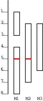
In the figure there are 6 tasks, with start times and finishing times (1,3), (2,5), (2,6), (4,5), (5,8), (5,7). They are scheduled on three machines M1, M2, M3. Clearly 3 machines are needed as can be seen by looking at time 4.
Note that a good solution to this problem has three objectives that must be met.
Let's illustrate the three objectives with following example
consisting of four tasks having starting and stopping times (1,3),
(6,8), (2,5), (4,7). It is easy to construct a wrong algorithm, for
example
Algorithm wrongTaskSchedule(T)
   Input:  A set T of tasks, each with start time si and
           finishing time fi (si≤fi).
   Output: A schedule of the tasks.

   while T is not empty do
      remove from T the first task and call it i.
      schedule i on M1
When applied to our 4-task example, the result is all four tasks assigned to machine 1. This is clearly infeasible since the last two tasks conflict.
It is also not hard to produce a poor algorithm, one that generates feasible, but non-optimal solutions.
Algorithm poorTaskSchedule(T):
   Input:  A set T of tasks, each with start time si and
   finishing time fi (si≤fi).
   Output: A feasible schedule of the tasks.

   m ← 0                         { current number of machines }
   while T is not empty do
      remove from T a task i
      m ← m+1
      schedule i on Mm
On the 4-task example, poorTaskSchedule puts each task on a different machine. That is certainly feasible, but is not optimal since the first and second task can go on one machine.
Hence it looks as though we should not put a task on a new machine if it can fit on an existing machine. That is certainly a greedy thing to do. Remember we are minimizing so being greedy really means being stingy. We minimize the number of machines at each step hoping that will give an overall minimum. Unfortunately, while better, this idea does not give optimal schedules. Let's call it mediocre.
Algorithm mediocreTaskSchedule(T):
   Input:  A set T of tasks, each with start time si and
   finishing time fi (si≤fi).
   Output: A feasible schedule of the tasks of T

   m ← 0                         { current number of machines }
   while T is not empty do
      remove from T a task i
      if there is an Mj having all tasks non-conflicting with i then
         schedule i on Mj
      else
         m ← m+1
         schedule i on Mm
When applied to our 4-task example, we get the first two tasks on one machine and the last two tasks on separate machines, for a total of 3 machines. However, a 2-machine schedule is possible, as we will shall soon see.
The needed new idea is to processes the tasks in order. Several orders would work, we shall order them by start time. If two tasks have the same start time, it doesn't matter which one is put ahead. For example, we could view the start and finish times as pairs and use lexicographical ordering. Alternatively, we could just sort on the first component.
Algorithm taskSchedule(T):
   Input:  A set T of tasks, each with start time si and
   finishing time fi (si≤fi).
   Output: An optimal schedule of the tasks of T

   m ← 0                         { current number of machines }
   while T is not empty do
      remove from T a task i with smallest start time
      if there is an Mj having all tasks non-conflicting with i then
         schedule i on Mj
      else
         m ← m+1
         schedule i on Mm
When applied to our 4-task example, we do get a 2-machine solution: the middle two tasks on one machine and the others on a second. But is this the minimum? Certainly for this example it is the minimum; we already saw that a 1-machine solution is not feasible. But what about other examples?
Assume the algorithm runs and declares m to be the minimum number of machines needed. We must show that m are really needed.
OK taskSchedule is feasible and optimal. But is it slow? That actually depends on some details of the implementation and it does require a bit of cleverness to get a fast solution.
Let N be the number of tasks in T. The book asserts that it is easy to see that the algorithm runs in time O(NlogN), but I don't think this is so easy. It is easy to see O(N2).