================ Start Lecture #20 ================
Skipped for now
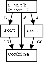
It is interesting to compare quick-sort with merge-sort. Both are divide and conquer algorithms. So we divide, recursively sort each piece, and then combine the sorted pieces.
In merge-sort, the divide is trivial: throw half the elements into one pile and the other half in another pile. The combine step, while easy does do comparisons and picks an element from the correct pile.
In quick-sort, the combine is trivial: pick up one pile, then the other. The divide uses comparisons to decide which pile each element should be placed into.
As usual we assume that the sequence we wish to sort contains no duplicates. It is easy to drop this condition if desired.
The book's algorithm does quick-sort in place, that is the sorted sequence overwrites the original sequence. Mine produces a new sorted sequence and leaves the original sequence alone.
Algorithm quick-sort (S)
   Input: A sequence S (of size n).
   Output: A sorted sequence T containing
           the same elements as S.

   if n < 2
      T ← S
      return

   Create empty sequences L and G { standing for less and greater }

   { Divide into L and G }
   Pick an element P from S { called the pivot }
   while (not S.isEmpty())
      x ← S.remove(S.first())
      if x < P then
         L.insertLast(x)
      if x > P then
         G.insertLast(x)

   { Recursively Sort L and G }
   LS ← quick-sort (L)    { LS stands for L sorted }
   GS ← quick-sort (G)

   { Combine LS, P, and GS }
   while (not LS.isEmpty())
      T.insertLast(LS.remove(LS.first()))
   T.insertLast(P)
   while (not GS.isEmpty())
      T.insertLast(GS.remove(GS.first()))
 The running time of quick sort is highly dependent on the choice of
the pivots at each stage of the recursion.
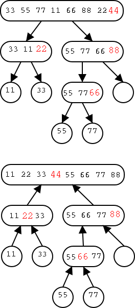
A very simple method is to choose the last element as the pivot.
This method is illustrated in the figure on the right. The pivot is
shown in red. This tree is not surprisingly called the
quick-sort tree.
The running time of quick sort is highly dependent on the choice of
the pivots at each stage of the recursion.
A very simple method is to choose the last element as the pivot.
This method is illustrated in the figure on the right. The pivot is
shown in red. This tree is not surprisingly called the
quick-sort tree.
The top tree shows the dividing and recursing that occurs with input {33,55,77,11,66,88,22,44}. The tree below shows the combining steps for the same input.
As with merge sort, we assign to each node of the tree the cost (i.e., running time) of the divide and combine steps. We also assign to the node the cost of the two recursive calls, but not their execution. How large are these costs?
The two recursive calls (not including the subroutine execution itself) are trivial and cost Θ(1).
The dividing phase is a simple loop whose running time is linear in the number of elements divided, i.e., in the size of the input sequence to the node. In the diagram this is the number of numbers inside the oval.
Similarly, the combining phase just does a constant amount of work per element and hence is again proportional to the number of elements in the node.
We would like to make an argument something like this. At each level of each of the trees the total number of elements is n so the cost per level is O(n). The pivot divides the list in half so the size of the largest node is divided by two each level. Hence the number of levels, i.e., the height of the tree, is O(log(n)). Hence the entire running time is O(nlog(n)).
That argument sound pretty good and perhaps we should try to make it more formal. However, I prefer to try something else since the argument is WRONG!
Homework:
Draw the quick-sort
tree for sorting the following sequence
{222 55 88 99 77 444 11 44 22 33 66 111 333}.
Assume the pivot is always the last element.
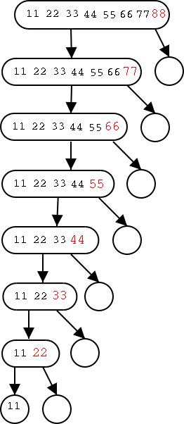 The tree on the right illustrates the worst case of quick-sort, which
occurs when the input is already sorted!
The tree on the right illustrates the worst case of quick-sort, which
occurs when the input is already sorted!
The height of the tree is N-1 not O(log(n)). This is because the pivot is in this case the largest element and hence does not come close to dividing the input into two pieces each about half the input size.
It is easy to see that we have the worst case. Since the pivot does not appear in the children, at least one element from level i does not appear in level i+1 so at level N-1 you can have at most 1 element left. So we have the highest tree possible. Note also that level i has at least i pivots missing so can have at most N-i elements in all the nodes. Our tree achieves this maximum. So the time needed is proportional to the total number of numbers written in the diagram which is N + N-1 + N-2 + ... + 1, which is again the one summation we know N(N+1)/2 or Θ(N2.
Hence the worst case complexity of quick-sort is quadratic! Why don't we call it slow sort?
Perhaps the problem was in choosing the last element as the pivot. Clearly choosing the first element is no better; the same example on the right again illustrates the worst case (the tree has its empty nodes on the left this time).
Since are spending linear time (as opposed to constant time) on the division step, why not count how many elements are present (say k) and choose element number k/2? This would not change the complexity (it is also linear). You could do that and now a sorted list is not the worst case. But some other list is. Just put the largest element in the middle and then put the second largest element in the middle of the node on level 1. This does have the advantage that if you mistakenly run quick-sort on a sorted list, you won't hit the worst case. But the worst case is still there and it is still Θ(N2).
Why not choose the real middle element as the pivot, i.e., the median. That would work! It would cut the sizes in half as desired. But how do we find the median? We could sort, but that is the original problem. In fact there is a (difficult) algorithm for computing the median in linear time and if this is used for the pivot, quick-sort does take O(Nlog(N)) time in the worst case. However, the difficult median algorithm is not fast in practice. That is, the constants hidden in saying it is Θ(N) are rather large.
Instead of studying the fast, difficult median algorithm, we will consider a randomized quick-sort algorithm and show that the expected running time is Θ(Nlog(N)).
Problem Set 4, Problem 2.
Find a sequence of size N=12 giving the worst case for quick-sort when
the pivot for sorting k elements is element number ⌊k/2⌋.
Consider running the following quick-sort-like experiment.
Are good splits rare or common?
Theorem: (From probability theory). The expected number of times that a fair coin must be flipped until it shows ``heads'' k times is 2k.
We will not prove this theorem, but will apply it to analyze good splits.
Theorem: The expected running time of randomized quick-sort on N numbers is O(Nlog(N)).
Proof: First we prove a little log lemma.
Lemma: logba = (log(a)) / log(b).
Proof of Lemma: First note that
alog(b) = blog(a) (take the log of both
sides).
Now raise each side to the power 1/log(b).
(alog(b))(1/log(b) =
(blog(a))1/log(b).
Thus a(log(b))/log(b) = b(log(a))/log(b)
(since (xy)z = xyz, see homework below).
So a = b(log(a))/log(b), which says that (log(a))/log(b) is the
power to which one raises b in order to get a. That is the definition of
logba.
End of Proof of Lemma
 Proof of Theorem:
We picked the pivot at random.
Therefore, if we imagine the
N numbers lined up in order, the pivot is equally likely to be
anywhere in this line.
Proof of Theorem:
We picked the pivot at random.
Therefore, if we imagine the
N numbers lined up in order, the pivot is equally likely to be
anywhere in this line.
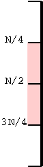
Consider the picture on the right. If the pivot is anywhere in the pink, the split is good. But the pink is half the line so the probability that we get a ``pink pivot'' (i.e., a good split) is 1/2. This is the same probability that a fair coin comes up heads.
Every good split divides the size of the node by at least 4/3. Recall that if you divide N by 4/3, log4/3(N) times, you will get 1. So the maximum number of good splits possible along a path from the root to a leaf is log4/3(N).
Applying the probability theorem above we see that the expected length of a path from the root to a leaf is at most 2log4/3(N). By the lemma this is (2log(N))/log(4/3), which is Θ(log(N)). That is, the expected height is O(log(N)).
Since the time spent at each level is O(N), the expected running time of randomized quick-sort is O(Nlog(N)). End of Proof of Theorem
Homework: Show that (xy)z = xyz. Hint take the log of both sides.
Theorem: The running time of any comparison-based sorting algorithm is Ω(Nlog(N)).
Proof: We will not cover this officially.
Unofficially, the idea is we form a binary tree with each node
corresponding to a comparison performed by the algorithm and the two
children corresponding to the two possible outcomes. This is a tree
of all possible executions (with only comparisons used for decisions).
There are N! permutations of N numbers and each must give a different
execution pattern in order to be sorted. So there are at least N!
leaves. Hence the height is at least log(N!). But N! has N/2
elements that are at least N/2 so N!≥(N/2)N/2. Hence
height ≥ log(N!) ≥ log((N/2)N/2) = (N/2)log(N/2)
So the running time, which is at least the height of this tree, is
Ω(Nlog(N))
Corollary: Heap-sort, merge-sort, and quick sort (with the difficult, linear-time, not-done-in-class median algorithm) are asymptotically optimal.