Separate chaining involves two data structures: the buckets and the log files. An alternative is to dispense with the log files and always store items in buckets, one item per bucket. Schemes of this kind are referred to as open addressing. The problem they need to solve is where to put an item when the bucket it should go into is already full? There are several different solutions. We study three: Linear probing, quadratic probing, and double hashing.
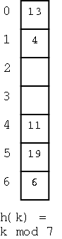
This is the simplest of the schemes. To insert a key k (really I should say ``to insert an item (k,e)'') we compute h(k) and initially assign k to A[h(k)]. If we find that A[h(k)] contains another key, we assign k to A[h(k)+1]. It that bucket is also full, we try A[h(k)+2], etc. Naturally, we do the additions mod N so that after trying A[N-1] we try A[0]. So if we insert (16,e) into the dictionary at the right, we place it into bucket 2.
How about finding a key k (again I should say an item (k,e))?
We first look at A[h(k)]. If this bucket contains the key, we have
found it. If not try A[h(k)+1], etc and of course do it mod N (I will
stop mentioning the mod N). So if
we look for 4 we find it in bucket 1 (after encountering two keys
that hashed to 6).
WRONG!
Or perhaps I should say incomplete. What if the item is not on
the list? How can we tell?
Ans: If we hit an empty bucket then the item is not present (if it
were present we would have stored it in this empty bucket). So 20
is not present.
What if the dictionary is full, i.e., if there are no empty
buckets.
Check to see if you have wrapped all the way around. If so, the
key is not present
What about removals?
Easy, remove the item creating an empty bucket.
WRONG!
Why?
I'm sorry you asked. This is a bit of a mess.
Assume we want to remove the (item with) key 19.
If we simply remove it, and search for 4 we will incorrectly
conclude that it is not there since we will find an empty slot.
OK so we slide all the items down to fill the hole.
WRONG! If we slide 6 into the whole at 5, we
will never be able to find 6.
So we only slide the ones that hash to 4??
WRONG! The rule is you slide all keys that are
not at their hash location until you hit an empty space.
Normally, instead of this complicated procedure for removals, we simple mark the bucket as removed by storing a special value there. When looking for keys we skip over such slots. When an insert hits such a bucket, the insert uses the bucket. (The book calls this a ``deactivated item'' object).
Homework: R-2.20
All the open addressing schemes work roughly the same. The difference is which bucket to try if A[h(k)] is full. One extra disadvantage of linear probing is that it tends to cluster the items into contiguous runs, which slows down the algorithm.
Quadratic probing attempts to spread items out by trying buckets A[h(k)], A[h(k)+1], A[h(k)+4], A[h(k)+9], etc. One problem is that even if N is prime this scheme can fail to find an empty slot even if there are empty slots.
Homework: R-2.21
In double hashing we have two hash functions h and h'. We use h as above and, if A[h(k)] is full, we try, A[h(k)+h'(k)], A[h(k)+2h'(k)], A[h(k)+3h'(k)], etc.
The book says h'(k) is often chosen to be q - (k mod q) for some prime q < N. I note again that if mod were defined correctly this would look more natural, namely (q-k) mod q. We will not consider which secondary hash function h' is good to use.
Homework: R-2.22
A hard choice. Separate chaining seems to use more space, but that is deceiving since it all depends on the loading factor. In general for each scheme the lower the loading factor, the faster scheme but the more memory it uses.
We just studied unordered dictionaries at the end of chapter 2. Now we want to extend the study to permit us to find the "next" and "previous" items. More precisely we wish to support, in addition to findElement(k), insertItem(k,e), and removeElement(k), the new methods
We naturally signal an exception if no such item exists. For example if the only keys present are 55, 22, 77, and 88, then closestKeyAfter(90) or closestElemBefore(2) each signal an exception.
We begin with the most natural implementation.
We use the sorted vector implementation from chapter 2 (we used it as a simple implementation of a priority queue). Recall that this keeps the items sorted in key order. Hence it is Θ(n) for inserts and removals, which is slow; however, we shall see that it is fast for finding and element and for the four new methods closestKeyBefore(k) and friends. We call this a lookup table.
The space required is Θ(n) since we grow and shrink the array supporting the vector (see extendable arrays).
As indicated the key favorable property of a lookup table is that it is fast for (surprise) lookups using the binary search algorithm that we study next.
In this algorithm we are searching for the rank of the item containing a key equal to k. We are to return a special value if no such key is found.
The algorithm maintains two variables lo and hi, which are respectively lower and upper bounds on the rank where k will be found (assuming it is present).
Initially, the key could be anywhere in the vector so we start with lo=0 and hi=n-1. We write key(r) for the key at rank r and elem(r) for the element at rank r.
We then find mid, the rank (approximately) halfway between lo and hi and see how the key there compares with our desired key.
Some care is need in writing the algorithm precisely as it is easy to have an ``off by one error''. Also we must handle the case in which the desired key is not present in the vector. This occurs when the search range has been reduced to the empty set (i.e., when lo exceeds hi).
Algorithm BinarySearch(S,k,lo,hi):
    Input:  An ordered vector S containing (key(r),elem(r)) at rank r
            A search key k
            Integers lo and hi
    Output: An element of S with key k and rank between lo and hi.
            NO_SUCH_KEY if no such element exits

If lo > hi then
    return NO_SUCH_KEY                    // Not present

mid ← ⌊(lo+hi)/2⌋
if k = key(mid) then
    return elem(mid)                     // Found it
if k < key(mid) then
    return BinarySearch(S,k,lo,mid-1)    // Try bottom ``half''
if k > key(mid) then
    return BinarySearch(S,k,mid+1,hi)    // Try top ``half''
Do some examples on the board.
It is easy to see that the algorithm does just a few operations per recursive call. So the complexity of Binary Search is Θ(NumberOfRecursions). So the question is "How many recursions are possible for a lookup table with n items?".
The number of eligible ranks (i.e., the size of the range we still must consider) is hi-lo+1.
The key insight is that when we recurse, we have reduced the range to at most half of what it was before. There are two possibilities, we either tried the bottom or top ``half''. Let's evaluate hi-lo+1 for the bottom and top half. Note that the only two possibilities for ⌊(lo+hi)/2⌋ are (lo+hi)/2 or (lo+hi)/2-(1/2)=(lo+hi-1)/2
Bottom:
(mid-1)-lo+1 = mid-lo = ⌊(lo+hi)/2⌋-lo
≤ (lo+hi)/2-lo = (hi-lo)/2 < (hi-lo+1)/2
Top:
hi-(mid+1)+1 = hi-mid = hi-⌊(lo+hi)/2⌋
≤ hi-(lo+hi-1)/2 = (hi-lo+1)/2
So the range starts at n and is halved each time and remains an integer (i.e., if a recursive call has a range of size x, the next recursion will be at most ⌊x/2⌋).
Write on the board 10 times
(X-1)/2 ≤ ⌊X/2⌋ &le X/2
If B ≤ A, then Z-A ≤ Z-B
How many recursions are possible? If the range is ever zero, we stop (and declare the key is not present) so the longest we can have is the number of times you can divide by 2 and stay at least 1. That number is Θ(log(n)) showing that binary search is a logarithmic algorithm.