Basic Algorithms

The Vector Representation of a Heap

Since we know that a heap is complete, it is efficient to use the vector representation of a binary tree. We can actually not bother with the leaves since we don't ever use them. We call the last node w (remember that is the last internal node). Its index in the vector representation is n, the number of keys in the heap. We call the first leaf z; its index is n+1. Node z is where we will insert a new element and is called the insertion position.

Insertion

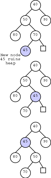
This looks trivial. Since we know n, we can find n+1 and hence the reference to node z in O(1) time. But there is a problem; the result might not be a heap since the new key inserted at z might be less than the key stored at u the parent of z. Reminiscent of bubble sort, we need to bubble the value in z up to the correct location.

Up-Heap Bubbling

We compare key(z) with key(u) and swap the items if necessary. In the diagram on the right we added 45 and then had to swap it with 70. But now 45 is still less than its parent so we need to swap again. At worst we need to go all the way up to the root. But that is only Θ(n) as desired. Let's slow down and see that this really works.

• We had a heap before we inserted the new element.
• When we insert the new element it can ruin the heap because it is too small (i.e. smaller than its parent),
• So the blue node is the problem.
• Since blue is smaller than its parent, we swap them. Call the parent the victim.
• Two nodes have been swapped we have four things to check: For each of these two nodes we must see that it is not larger than its new children and not smaller than its new parent.
  1. The blue node is definitely not larger than its new children: One child is the victim, which we know is larger than the blue. The other child was not smaller than the victim so is surely not smaller than the blue.
  2. The blue node might be smaller than its new parent. Indeed in the diagram on the right it is. That is why we have to keep bubbling up.
  3. Before we did the insert, we had a heap so at that point the victim was not larger than all its descendents. But after the swap, all of the children of the victim were descendents of the victim before.
  4. The victim is definitely not smaller than its new parent, which is the blue.

Great. It works (i.e., is a heap) and there can only be O(log(n)) swaps because that is the height of the tree.

But wait! What I showed is that it only takes O(n) steps. Is each step O(1)?

Comparing is clearly O(1) and swapping two fixed elements is also O(1). Finding the parent of a node is easy (integer divide the vector index by 2). Finally, it is trivial to find the new index for the insertion point (just increase the insertion point by 1).

Remark: It is not as trivial to find the new insertion point using a linked implementation.

Homework: Show the steps for inserting an element with key 2 in the heap of Figure 2.41.

Removal

Trivial, right? Just remove the root since that must contain an element with minimum key. Also decrease n by one.
Wrong!
What remains is TWO trees.

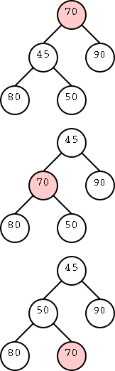
We do want the element stored at the root but we must put some other element in the root. The one we choose is our friend the last node.

But the last node is likely not to be a valid root, i.e. it will destroy the heap property since it will likely be bigger than one of its new children. So we have to bubble this one down. It is shown in pale red on the right and the procedure explained below. We also need to find a new last node, but that really is trivial: It is the node stored at the new value of n.

Down-Heap Bubbling

If the new root is the only internal node then we are done.

If only one child of the root is internal (it must be the left child) compare its key with the key of the root and swap if needed.

If both children of the root are internal, choose the child with the smaller key and swap with the root if needed.

The original last node, became the root, and now has been bubbled down to level 1. But it might still be bigger than a child so we keep bubbling. At worst we need Θ(h) bubbling steps, which is again logarithmic in n as desired.

Homework: R-2.16

Operation	Time
size, isEmpty	O(1)
minElement, minKey	O(1)
insertItem	Θ(log n)
removeMin	Θ(log n)

Performance

The table on the right gives the performance of the heap implementation of a priority queue. As desired, the main operations have logarithmic time complexity. It is for this reason that heap sort is fast.

Summary of heaps

• A heap containing n elements is a complete tree T with n internal nodes each storing a reference to a key and a reference to an element. The tree also contains n+1 leaves, which are not used.
  
  
• The heap is a very fast implementation of a priority queue. The main operations are logarithmic and the others are constant time.
  • The height of the heap is Θ(log(n)) since T is complete.
  • The worst case complexity of the up- and down-heap bubbling are Θ(height)=Θ(log(n)).
  • Finding the insertion position and updating the last node position take constant time.
  • The insertItem and removeMin operations are Θ(log(n)). So are minItem and minKey
  
  
• Using these insertion and removeMin algorithms makes sorting using a priority queue fast, i.e., Θ(n*log(n)), as we shall state officially in the next section.

2.4.4 Heap-Sort (and some extras)

The goal is to sort a sequence S. We return to the PQ-sort where we insert the elements of S into a priority queue and then use removeMin to obtain the sorted version. When we use a heap to implement the priority queue, each insertion and removal takes Θ(log(n)) so the entire algorithm takes Θ(nlog(n)). The heap implementation of PQ-sort is called heap-sort and we have shown

Theorem: The heap-sort algorithm sorts a sequence of n comparable elements in Θ(nlog(n)) time.

Implementing Heap-Sort In Place

In place means that we use the space occupied by the input. More precisely, it means that the space required is just the input + O(1) additional memory. The algorithm above required Θ(n) addition space to store the heap.

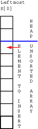
The in place heap-sort of S assumes that S is implemented as an array and proceeds as follows (This presentation, beyond the definition of ``in place'' is unofficial; i.e., it will not appear on problem sets or exams)

1. Logically divide the array into a portion in the front that contains the growing heap and the rest that contains the elements of the array that have not yet been dealt with.
   • Initially the heap part is empty and the not-yet-dealt-with part of the array is the entire array.
   • At each insertion we remove the left most entry from the array part and insert it in the heap, growing the heap to include the memory previously used by the newly inserted element. The blue line moves down.
   • At the end the heap uses all the space. We are making the optimization discussed before that we only store the internal nodes of the heap and do not waste the first (index 0) component of the array used to store the heap.
2. Do the insertions a with a normal heap-sort but change the comparison so that a maximum element is in the root (i.e., a parent is no smaller than a child).
3. Now do the removals from the heap, moving the blue line back up.
   • The elements removed are in order big to small.
   • This is perfect since we are going to store them starting at the right of the array since that is the portion of the array that is made available by the shrinking heap.

Bottom-Up Heap Constructor (unofficial)

If you are given at the beginning all n elements that are to be inserted, the total insertion time for all inserts can be reduced to O(n) from O(nlog(n)). The basic idea assuming n=2ⁿ-1 is

1. Take out the first element and call it r.
2. Divide the remaining 2ⁿ-2 into two parts each of size 2^n-1-1.
3. Heap-sort each of these two parts.
4. Make a tree with r as root and the two heaps as children.
5. Down-heap bubble r.

Locaters (Unofficial)

Sometimes we wish to extend the priority queue ADT to include a locater that always points to the same element even when the element moves around. So if x is in a priority queue and another item is inserted, x may move during the up-heap bubbling, but the locater of x continues to refer to x.

Comparison of the Priority Queue Implementations

Method	Unsorted Sequence	Sorted Sequence	Heap
size, isEmpty	Θ(1)	Θ(1)	Θ(1)
minElement, minKey	Θ(n)	Θ(1)	Θ(1)
insertItem	Θ(1)	Θ(n)	Θ(log(n))
removeMin	Θ(n)	Θ(1)	Θ(log(n))