 Definition: A binary tree of height h is
complete if the levels 0,...,h-1 contain the maximum
number of elements and on level h-1 all the internal nodes are to the
left of all the leaves.
Definition: A binary tree of height h is
complete if the levels 0,...,h-1 contain the maximum
number of elements and on level h-1 all the internal nodes are to the
left of all the leaves.
================ Start Lecture #10 ================
However, this implementation can waste a lot of space since many of the entries in S might be unused. That is there may be many i for which S[i] is null.
Problem Set 2 problem 3. Give a tree with fewer than 20 nodes for which S.size() exceeds 100. Give a tree with fewer than 25 nodes for which S.size() exceeds 1000. Give a tree with fewer than 100 nodes for which S.size() exceeds a million.
Represent each node by a quadruple.
Once again the algorithms are all O(1) except for positions() and elements(), which are Θ(n).
The space is Θ(n) which is much better that for the vector implementation. The constant is larger however since three pointers are stored for each position rather than one index.
The only difference is that we don't know how many children each node has. We could store k child pointers and say that we cannot process a tree having more than k children with the same parent.
Clearly we don't like this limit. Moreover, if we choose k moderate, say k=10. We are limited to 10-ary trees and for 3-ary trees most of the space is wasted.
So instead of storing the child references in the node, we store just one reference to a container. The container has references to the children. Imagine implementing the container as an extendable array.
Since a node v contains an arbitrary number of children, say Cv, the complexity of the children(v) iterator is Θ(Cv).
Up to now we have not considered elements that must be retrieved in a fixed order. But often in practice we assign a priority to each item and want the most important (highest priority) item first. (For some reason that I don't know, low numbers are often used to represent high priority.)
For example consider processor scheduling from Operating Systems (202). The simplest scheduling policy is FCFS for which a queue of ready processors is appropriate. But if we want SJF (short job first) then we want to extract the ready process that has the smallest remaining time. Hence a FIFO queue is not appropriate.
For a non-computer example,consider managing your todo list. When you get another item to add, you decide on its importance (priority) and then insert the item into the todo list. When it comes time to perform an item, you want to remove the highest priority item. Again the behavior is not FIFO.
To return items in order, we must know when one item is less than another. For real numbers this is of course obvious.
We assume that each item has a key on which the priority is to be based. For the SJF example given above, the key is the time remaining. For the todo example, the key is the importance.
We assume the existence of an order relation (often called a total order) written ≤ satisfying for all keys s, t, and u.
Remark: For the complex numbers no such ordering exists that extends the natural ordering on the reals and imaginaries. This is unofficial (not part of 310).
Is it OK to define s≤t for all s and t?
No. That would not be antisymmetric.
Definition: A priority queue is a container of elements each of which has an associated key supporting the following methods.
Users may choose different comparison functions for the same data. For example, if the keys are longitude,latitude pairs, one user may be interested in comparing longitudes and another latitudes. So we consider a general comparator containing methods.
Given a priority queue it is trivial to sort a collection of elements. Just insert them and then do removeMin to get them in order. Written formally this is
Algorithm PQ-Sort(C,P)
   Input: an n element sequence C and an empty priority queue P
   Output: C with the elements sorted

   while not C.isEmpty() do
      e←C.removeFirst()
      P.insertItem(e,e)  // We are sorting on the element itself.

   while not P.isEmpty()
      C.insertLast(P.removeMin())
So whenever we give an implementation of a priority queue, we are also giving a sorting algorithm. Two obvious implementations of a priority queue give well known (but slow) sorts. A non-obvious implementation gives a fast sort. We begin with the obvious.
So insertItem() takes Θ(1) time and hence takes Θ(N) to insert all n items of C. But remove min, requires we go through the entire list. This requires time Θ(k) when there are k items in the list. Hence to remove all the items requires Θ(n+(n-1)+...+1) = Θ(N2) time.
This sorting algorithm is normally called selection sort since the dominant step is selecting the minimum each time.
Now removeMin() is trivial since it is just removeFirst(). But insertItem is Θ(k) when there are k items already in the priority queue since you must step through to find the correct location to insert and then slide the remaining elements over.
This sorting algorithm is normally called insertion sort since the dominant effort is inserting each element.
We now consider the non-obvious implementation of a priority queue
that gives a fast sort (and a fast priority queue).
The idea is to use a tree to store the elements, with the smallest
element stored in the root.
We will store elements only in the internal nodes (i.e., the leaves
are not used). One could imagine an implementation in which the leaves
are not even implemented since they are not used.
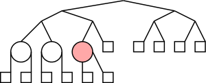
We follow the book and draw internal nodes as circles and leaves
(i.e., external nodes) as squares.
Since the priority queue algorithm will perform steps with complexity
Θ(height of tree), we want to keep the height small.
The way to do this is to fully use each level.
Definition: A binary tree of height h is
complete if the levels 0,...,h-1 contain the maximum
number of elements and on level h-1 all the internal nodes are to the
left of all the leaves.
Remarks:
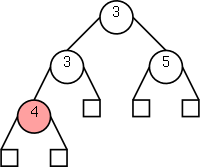
Definition: A tree storing a key at each internal node satisfies the heap-order property if, for every node v other than the root, the key at v is no smaller than the key at v's parent.
Definition: A heap is a complete binary tree satisfying the heap order property.
Definition: The last node of a heap is the right most internal node in level h-1. In the diagrams above the last nodes are pink.
Remark: As written the ``last node'' is really the
last internal node. However, we actually don't use the leaves to
store keys so in some sense ``last node'' is the last (significant) node.
Homework:
With a heap it is clear where the minimum is located, namely at the root. We will also use a reference to the last node since insertions will occur at the first node after last.
Theorem: A heap storing n keys has height ⌈log(n+1)⌉
Proof:
Corollary: If we can implement insert and removeMin in time Θ(height), we will have implemented the priority queue operations in logarithmic time (our goal).
Illustrate the theorem with the diagrams above.