================ Start Lecture #1 ================
Operating Systems
2002-2003 Fall
Monday 5-6:50
Ciww 109
Chapter -1: Administrivia
I start at -1 so that when we get to chapter 1, the numbering will
agree with the text.
(-1).1: Contact Information
- gottlieb@nyu.edu (best method)
- http://allan.ultra.nyu.edu/~gottlieb two el's in allan
- 715 Broadway, Room 712
(-1).2: Course Web Page
There is a web site for the course. You can find it from my home
page, which is http://allan.ultra.nyu.edu/~gottlieb
- You can find these lecture notes on the course home page.
Please let me know if you can't find it.
- I mirror my home page on the CS web site.
- I also mirror the course pages on the CS web site.
- But, the official site is allan.ultra.nyu.edu.
It is the one I personally manage.
- The notes will be updated as bugs are found.
- I will also produce a separate page for each lecture after the
lecture is given. These individual pages
might not get updated as quickly as the large page
(-1).3: Textbook
The course text is Tanenbaum, "Modern Operating Systems", 2nd Edition
- The first edition is not adequate as there have been many
changes.
- Available in bookstore.
- We will cover nearly all of the first 6 chapters.
(-1).4: Computer Accounts and Mailman Mailing List
- You are entitled to a computer account, please get it asap.
- Sign up for the Mailman mailing list for the course.
http://www.cs.nyu.edu/mailman/listinfo/G22_2250_001_fa02
- If you want to send mail just to me, use gottlieb@nyu.edu not
the mailing list.
- Questions on the labs should go to the mailing list.
You may answer questions posed on the list as well.
- I will respond to all questions; if another student has answered the
question before I get to it, I will confirm if the answer given is
correct.
(-1).5: Grades
Assuming 3 labs, which is likely, grades will computed as
.3*LabAverage + .7*FinalExam (but see homeworks below).
(-1).6: No Midterm Exam
(-1).7: Homeworks and Labs
I make a distinction between homeworks and labs.
Labs are
- Required.
- Due several lectures later (date given on assignment).
- Graded and form part of your final grade.
- Penalized for lateness.
- Computer programs you must write.
Homeworks are
- Optional.
- Due the beginning of Next lecture.
- Not accepted late.
- Mostly from the book.
- Collected and returned.
- Able to help, but not hurt, your grade.
(-1).7.1: Doing Labs on non-NYU Systems
You may solve lab assignments on any system you wish, but ...
- You are responsible for any non-nyu machine.
I extend deadlines if the nyu machines are down, not if yours are.
- Be sure to upload your assignments to the
nyu systems.
- In an ideal world, a program written in a high level language
like Java, C, or C++ that works on your system would also work
on the NYU system used by the grader.
Sadly this ideal is not always achieved despite marketing
claims that it is achieved.
So, although you may develop you lab on any system,
you must ensure that it runs on the nyu system assigned to the
course.
- If somehow your assignment is misplaced by me and/or a grader,
we need a to have a copy ON AN NYU SYSTEM
that can be used to verify the date the lab was completed.
- When you complete a lab (and have it on an nyu system), do
not edit those files. Indeed, put the lab in a separate
directory and keep out of the directory. You do not want to
alter the dates.
(-1).7.2: Obtaining Help with the Labs
Good methods for obtaining help include
- Asking me during office hours (see web page for my hours).
- Asking the mailing list.
- Asking another student, but ...
Your lab must be your own.
That is, each student must submit a unique lab.
Naturally changing comments, variable names, etc does
not produce a unique lab
(-1).8: The Upper Left Board
I use the upper left board for lab/homework assignments and
announcements. I should never erase that board.
Viewed as a file it is group readable (the group is those in the
room), appendable by just me, and (re-)writable by no one.
If you see me start to erase an announcement, let me know.
(-1).9: A Grade of ``Incomplete''
It is university policy that a student's request for an incomplete
be granted only in exceptional circumstances and only if applied for
in advance. Naturally, the application must be before the final exam.
Chapter 0: Interlude on Linkers
Originally called a linkage editor by IBM.
A linker is an example of a utility program included with an
operating system distribution. Like a compiler, the linker is not
part of the operating system per se, i.e. it does not run in supervisor mode.
Unlike a compiler it is OS dependent (what object/load file format is
used) and is not (normally) language dependent.
0.1: What does a Linker Do?
Link of course.
When the compiler and assembler have finished processing a module,
they produce an object module
that is almost runnable.
There are two remaining tasks to be accomplished for the object module
to be runnable.
Both are involved with linking (that word, again) together multiple
object modules.
The tasks are relocating relative addresses
and resolving external references.
0.1.1: Relocating Relative Addresses
- Each module is (mistakenly) treated as if it will be loaded at
location zero.
- For example, the machine instruction
jump 100
is used to indicate a jump to location 100 of
the current module.
- To convert this relative address to an
absolute address,
the linker adds the base address of the module
to the relative address.
The base address is the address at which
this module will be loaded.
- Example: Module A is to be loaded starting at location 2300 and
contains the instruction
jump 120
The linker changes this instruction to
jump 2420
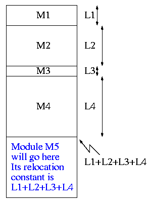
- How does the linker know that Module M5 is to be loaded starting at
location 2300?
- It processes the modules one at a time. The first module is
to be loaded at location zero.
So relocating is trivial
(adding zero).
We say that the relocation constant is zero.
- After processing the first module, the linker knows its length
(say that length is L1).
- Hence the next module is to be loaded starting at L1, i.e.,
the relocation constant is L1.
- In general the linker keeps the sum of the lengths of
all the modules it has already processed; this sum is the
relocation constant for the next module.
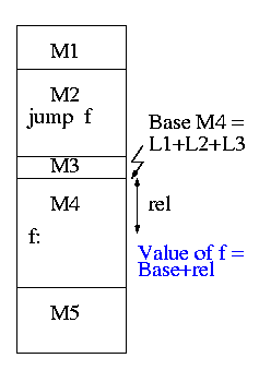
0.1.2: Resolving External Reverences
- If a C (or Java, or Pascal) program contains a function call
f(x)
to a function f() that is compiled separately, the resulting
object module must contain some kind of jump to the beginning of
f.
- But this is impossible!
- When the C program is compiled. the compiler and assembler
do not know the location of f() so there is no
way they can supply the starting address.
- Instead a dummy address is supplied and a notation made that
this address needs to be filled in with the location of
f(). This is called a use of
f.
- The object module containing the definition
of f() contains a notation
that f is being defined and gives the relative address of the
definition, which the linker can convert to an absolute address.
- The linker then changes all uses of f() to the correct absolute address.
The output of a linker is called a load module
because it is now ready to be loaded and run.
To see how a linker works lets consider the following example,
which is the first dataset from lab #1. The description in lab1 is
more detailed.
The target machine is word addressable and has a memory of 250
words, each consisting of 4 decimal digits. The first (leftmost)
digit is the opcode and the remaining three digits form an address.
Each object module contains three parts, a definition list, the
program text itself, and a use list. Each definition is a pair (sym,
loc). Each use is a symbol.
The program text consists of a count N followed by N pairs (type, word),
where word is a 4-digit instruction described above and type is a
single character indicating if the address in the word is
Immediate,
Absolute,
Relative, or
External.
Input set #1

1 xy 2
2 z xy
5 R 1004  I 5678  E 2000  R 8002  E 7001
0
1 z
6 R 8001  E 1000  E 1000  E 3000  R 1002  A 1010
0
1 z
2 R 5001  E 4000
1 z 2
2 xy z
3 A 8000  E 1001  E 2000
The first pass simply finds the base address of each module and
produces the symbol table giving the values for xy and z (2 and 15
respectively). The second pass does the real work using the symbol
table and base addresses produced in pass one.
              Symbol Table
                  xy=2
                  z=15

               Memory Map
 +0
 0:       R 1004      1004+0 = 1004
 1:       I 5678               5678
 2: xy:   E 2000 ->z           2015
 3:       R 8002      8002+0 = 8002
 4:       E 7001 ->xy          7002
 +5
 0        R 8001      8001+5 = 8006
 1        E 1000 ->z           1015
 2        E 1000 ->z           1015
 3        E 3000 ->z           3015
 4        R 1002      1002+5 = 1007
 5        A 1010               1010
 +11
 0        R 5001      5001+11= 5012
 1        E 4000 ->z           4015
 +13
 0        A 8000               8000
 1        E 1001 ->z           1015
 2 z:     E 2000 ->xy          2002
(Unofficial) Remark:
It is faster (less I/O) to do a one pass approach, but is harder
since you need ``fix-up code'' whenever a use occurs in a module that
precedes the module with the definition.
The linker on unix is mistakenly called ld (for loader), which is
unfortunate since it links but does not load.
Lab #1:
Implement a linker. The specific assignment is detailed on the sheet
handed out in in class and is due in three weeks. The
content of the handout is available on the web as well (see the class
home page).
End of Interlude on Linkers
Chapter 1: Introduction
Homework: Read Chapter 1 (Introduction)
Levels of abstraction (virtual machines)
- Software (and hardware, but that is not this course) is often
implemented in layers.
- The higher layers use the facilities provided by lower layers.
- Alternatively said, the upper layers are written using a more
powerful and more abstract virtual machine than the lower layers.
- Alternatively said, each layer is written as though it runs on the
virtual machine supplied by the lower layer and in turn provides a more
abstract (pleasant) virtual machine for the higher layer to run on.
- Using a broad brush, the layers are.
- Applications and utilities
- Compilers, Editors, Command Interpreter (shell, DOS prompt)
- Libraries
- The OS proper (the kernel, runs in
privileged/kernel/supervisor mode)
- Hardware
- Compilers, editors, shell, loader. etc run in user mode.
- The kernel itself is itself normally layered, e.g.
- ...
- Filesystems
- Machine independent I/O
- Machine dependent device drivers
- The machine independent I/O part is written assuming ``virtual
(i.e. idealized) hardware''. For example, the machine independent I/O
portion simply reads a block from a ``disk''. But
in reality one must deal with the specific disk controller.
- Often the machine independent part is more than one layer.
- The term OS is not well defined. Is it just the kernel? How
about the libraries? The utilities? All these are certainly
system software but not clear how much is part of the OS.
================ Start Lecture #2 ================
1.1: What is an operating system?
The kernel itself raises the level of abstraction and hides details.
For example a user (of the kernel) can write to a file (a concept not
present in hardware) and ignore whether the file resides on a floppy,
a CD-ROM, or a hard magnetic disk
The kernel is a resource manager (so users don't conflict).
How is an OS fundamentally different from a compiler (say)?
Answer: Concurrency! Per Brinch Hansen in Operating Systems
Principles (Prentice Hall, 1973) writes.
The main difficulty of multiprogramming is that concurrent activities
can interact in a time-dependent manner, which makes it practically
impossibly to locate programming errors by systematic testing.
Perhaps, more than anything else, this explains the difficulty of
making operating systems reliable.
Homework: 1, 2. (unless otherwise stated, problems
numbers are from the end of the chapter in Tanenbaum.)
1.2 History of Operating Systems
- Single user (no OS).
- Batch, uniprogrammed, run to completion.
- The OS now must be protected from the user program so that it is
capable of starting (and assisting) the next program in the batch).
- Multiprogrammed
- The purpose was to overlap CPU and I/O
- Multiple batches
- IBM OS/MFT (Multiprogramming with a Fixed number of Tasks)
- OS for IBM system 360.
- The (real) memory is partitioned and a batch is
assigned to a fixed partition.
- The memory assigned to a
partition does not change.
- Jobs were spooled from cards into the
memory by a separate processor (an IBM 1401).
Similarly output was
spooled from the memory to a printer (I believe a
1403) by the 1401.
- IBM OS/MVT (Multiprogramming with a Variable number of Tasks)
(then other names)
- Each job gets just the amount of memory it needs. That
is, the partitioning of memory changes as jobs enter and leave
- MVT is a more ``efficient'' user of resources but is
more difficult.
- When we study memory management, we will see that with
varying size partitions questions like compaction and
``holes'' arise.
- Time sharing
- This is multiprogramming with rapid switching between jobs
(processes). Deciding when to switch and which process to
switch to is called scheduling.
- We will study scheduling when we do processor management
- Personal Computers
- Serious PC Operating systems such as linux, Windows NT/2000/XP
and (the newest) MacOS are multiprogrammed OSes.
- GUIs have become important. Debate as to whether it should be
part of the kernel.
- Early PC operating systems were uniprogrammed and their direct
descendants still are (e.g. Windows ME).
Homework: 3.
1.3: OS Zoo
There is not as much difference between mainframe, server,
multiprocessor, and PC OSes as Tannenbaum suggests. For example
Windows NT/2000/XP are used in all (except mainframes) and Unix and
Linux are used on all.
1.3.1: Mainframe Operating Systems
Used in data centers, these systems ofter tremendous I/O
capabilities.
1.3.2: Server Operating Systems
Perhaps the most important servers today are web servers.
Again I/O (and network) performance are critical.
1.3.3: Multiprocessor Operating systems
These existed almost from the beginning of the computer
age, but now are not exotic.
1.3.4: PC Operating Systems (client machines)
Some OSes (e.g. Windows ME) are tailored for this application. One
could also say they are restricted to this application.
1.3.5: Real-time Operating Systems
- Often are Embedded Systems.
- Soft vs hard real time. In the latter missing a deadline is a
fatal error--sometimes literally.
- Very important commercially, but not covered much in this course.
1.3.6: Embedded Operating Systems
- The OS is ``part of'' the device. For example, PDAs,
microwave ovens, cardiac monitors.
- Often are real-time systems.
- Very important commercially, but not covered much in this course.
1.3.7: Smart Card Operating Systems
Very limited in power (both meanings of the word).
Multiple computers
- Network OS: Make use of the multiple PCs/workstations on a LAN.
- Distributed OS: A ``seamless'' version of above.
- Not part of this course (but often in G22.2251).
Homework: 5.
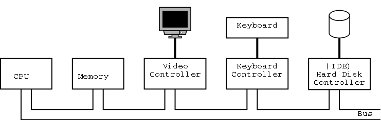
1.4: Computer Hardware Review
Tannenbaum's treatment is very brief and superficial. Mine is even
more so.
The picture on the right is very simplified.
For one thing, today separate buses are used to Memory and Video.
1.4.1: Processors
We will ignore processor concepts such as program
counters and stack pointers. We will also ignore
computer design issues such as pipelining and
superscalar. We do, however, need the notion of a
trap, that is an instruction that atomically
switches the processor into privileged mode and jumps to a pre-defined
physical address.
1.4.2: Memory
We will ignore caches, but will (later) discuss demand paging,
which is very similar although uses completely disjoint terminology.
In both cases, the goal is to combine large slow memory with small
fast memory and achieve the effect of large fast memory.
The central memory in a system is called RAM
(Random Access Memory). A key point is that it is volatile, i.e. the
memory loses its value if power is turned off.
Disk Hardware
I don't understand why Tanenbaum discusses disks here instead of in
the next section entitled I/O devices, but he does. I don't.
ROM / PROM / EPROM / EEPROM / Flash Ram
ROM (Read Only Memory) is used to hold data that
will not change, e.g. the serial number of a computer or the program
use in a microwave. ROM is non-volatile.
But often this unchangable data needs to be changed (e.g., to fix
bugs). This gives rise first to PROM (Programmable ROM), which, like a
CD-R, can be written once (as opposed to being mass produced already
written like a CD-ROM), and then to EPROM (Erasable PROM; not Erasable
ROM as in Tanenbaum), which is like a CD-RW. An EPROM is especially.
convenient if it can be erased with a normal circuit (EEPROM,
Electrically EPROM or Flash RAM).
Memory Protection and Context Switching
As mentioned above when discussing
OS/MFT and OS/MVT
multiprogramming requires that we protect one process from another.
That is we need to translate the virtual addresses of
each program into distinct physical addresses. The
hardware that performs this translation is called the
MMU or Memory Management Unit.
When context switching from one process to
another, the translation must change, which can be an expensive
operation.
1.4.3: I/O Devices
When we do I/O for real, I will show a real disk opened up and
illustrate the components
- Platter
- Surface
- Head
- Track
- Sector
- Cylinder
- Seek time
- Rotational latency
- Transfer time
Devices are often quite complicated to manage and a separate
computer, called a controller, is used to translate simple commands
(read sector 123456) into what the device requires (read cylinder 321,
head 6, sector 765). Actually the controller does considerably more,
e.g. calculates a checksum for error detection.
How does the OS know when the I/O is complete?
- It can busy wait constantly asking the controller
if the I/O is complete. This is the easiest (by far) but has low
performance. It is also called polling or
PIO (Programmed I/O).
- It can tell the controller to start the I/O and then switch to
other tasks. The controller must then interrupt
the OS when the I/O is done. Less waiting, but harder
(concurrency!).
- Some controllers can do
DMA (Direct Memory Access)
in which case they deal directly with memory after being started
by the CPU. This takes work from the CPU and halves the number of
bus accesses.
We discuss this more in chapter 5. In particular, we explain the last
point about halving bus accesses there.
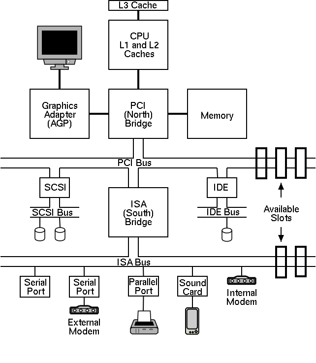
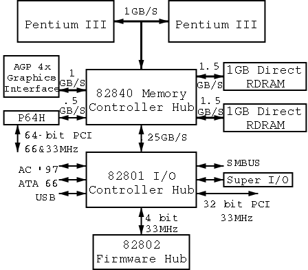
1.4.3: Buses
I don't care so much about the names of the buses, but the diagram
given in the book doesn't show a modern design. The one on the right
does. Below is a figure showing the specifications for a modern chip
set (introduced in 2000).
1.5: Operating System Concepts
This will be very brief. Much of the rest of the course will consist in
``filling in the details''.
1.5.1: Processes
A program in execution. If you run the same program twice, you have
created two processes. For example if you have two editors running in
two windows, each instance of the editor is a separate process.
Often one distinguishes the state or context (memory image, open
files) from the thread of control. Then if one has many
threads running in the same task, the result is a
``multithreaded processes''.
The OS keeps information about all processes in the process
table.
Indeed, the OS views the process as the entry.
This is an example of an active entity being viewed as a data structure
(cf. discrete event simulations).
An observation made by Finkel in his (out of print) OS textbook.
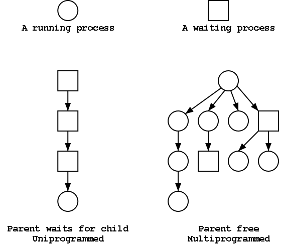
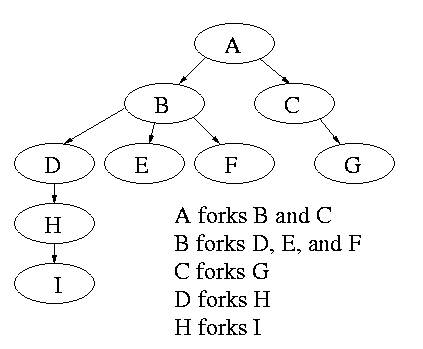
The set of processes forms a tree via the fork system call. The
forker is the parent of the forkee, which is called a
child. If the system blocks the parent until
the child finishes, the ``tree'' is quite simple, just a line. But
the parent (in many OSes) is free to continue executing and in
particular is free to fork again producing another child.
A process can send a signal to another process to
cause the latter to
execute a predefined function (the signal handler).
This can be tricky to program since the programmer does not know when
in his ``main'' program the signal handler will be invoked.
Each user is assigned User IDentification (UID)
and all processes created by that user have this UID.
One UID is special (the superuser or
administrator) and has extra privileges.
A child has the same UID as its parent. It is sometimes possible to
change the UID of a running process. A group of users can be formed
and given a Group IDentification, GID.
Access to files and devices can be limited to a given UID or GID.
================ Start Lecture #3 ================

1.5.2: Deadlocks
A set of processes each of which is blocked by a process in the
set. The automotive equivalent, shown at right, is gridlock.
1.5.3: Memory Management
Each process requires memory. The loader produces a load module
that assumes the process is loaded at location 0. The operating
system ensures that the processes are actually given disjoint
memory. Current operating systems permit each process to be
given more (virtual) memory than the
total amount of (real) memory on the
machine.
1.5.4: Input/Output
There are a wide variety of I/O devices that the OS must manage.
For example, if two processes are printing at the same time, the OS
must not interleave the output. The OS contains device
specific code (drivers) for each device as well as device-independent
I/O code.
1.5.5: Files
Modern systems have a hierarchy of files. A file system tree.
- In MSDOS the hierarchy is a forest not a tree. There is no file,
or directory that is an ancestor of both a:\ and c:\.
- In unix the existence of (hard) links weakens the tree to a DAG.
- Unix also has symbolic links, which when used indiscriminately,
permit directed cycles (i.e., the result is not a DAG).
You can name a file via an absolute path starting
at the root directory or via a relative path starting
at the current working directory.
In addition to regular files and directories, Unix also uses the
file system namespace for devices
(called special files, which
are typically found in the /dev
directory. Often utilities that are normally applied to (ordinary)
files can be applied as well to some special files. For example, when
you are accessing a unix system using a mouse and do not have anything
serious going
on (e.g., right after you log in), type the following command
cat /dev/mouse
and then move the mouse. You kill the cat by typing cntl-C. I tried
this on my linux box and no damage occurred. Your mileage may vary.
Before a file can be accessed, it must be opened
and a file descriptor obtained.
Many systems have standard files that are automatically made available
to a process upon startup. These (initial) file descriptors are fixed
- standard input: fd=0
- standard output: fd=1
- standard error: fd=2
A convenience offered by some command interpretors is a pipe or
pipeline. The pipeline
dir | wc
which pipes the output dir into a character/word/line counter,
will give the number of files in the directory (plus other info).
1.5.6: Security
Files and directories normally have permissions
- Normally have at least rwx.
- User, group, world
- A more general mechanism is an
access control lists.
- Often files have ``attributes'' as well. For example the linux ext2
file system supports a ``d'' attribute that is a hint to
the dump program not to backup this file.
- When a file is opened, permissions are checked and, if the open is
permitted, a file descriptor is
returned that is used for subsequent operations
1.5.7: The Shell or Command Interpreter (DOS Prompt)
The command line interface to the operating system. The shell
permits the user to
- Invoke commands
- Pass arguments to the commands
- Redirect the output of a command to a file or device
- Pipe one command to another (as illustrated above via ls | wc)
Homework: 8
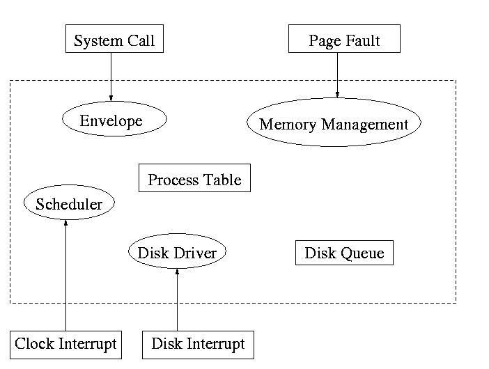
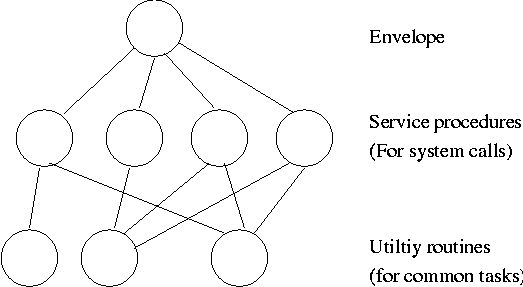
1.6: System Calls
System calls are the way a user (i.e., a program)
directly interfaces with the OS. Some textbooks use the term
envelope for the component of the OS responsible for fielding
system calls and dispatching them. On the right is a picture showing
some of the OS components and the external events for which they are
the interface.
Note that the OS serves two masters. The hardware (below)
asynchronously sends interrupts and the user makes system
calls and generates page faults.
Homework: 14
What happens when a user executes a system call such as read()?
We show a more detailed picture below, but at a high level what
happens is
- Normal function call (in C, Ada, Pascal, etc.).
- Library routine (in C).
- Small assembler routine.
- Move arguments to predefined place (perhaps registers).
- Poof (a trap instruction) and then the OS proper runs in
supervisor mode.
- Fix up result (move to correct place).
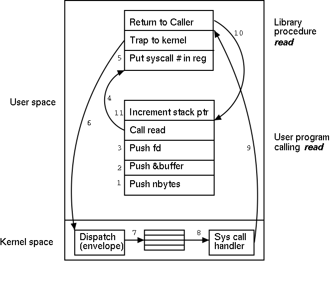 The following actions occur when the user executes the (Unix)
system call
The following actions occur when the user executes the (Unix)
system call
count = read(fd,buffer,nbytes)
which reads up to
nbytes from the file described by fd into buffer. The actual number
of bytes read is returned (it might be less than nbytes if, for
example, an eof was encountered).
- Push third parameter on to the stack.
- Push second parameter on to the stack.
- Push first parameter on to the stack.
- Call the library routine, which involves pushing the return
address on to the stack and jumping to the routine.
- Machine/OS dependent actions. One is to put the system call
number for read in a well defined place, e.g., a specific
register. This requires assembly language.
- Trap to the kernel (assembly language). This enters the operating
system proper and shifts the computer to privileged mode.
- The envelope uses the system call number to access a table of
pointers to find the handler for this system call.
- The read system call handler processes the request (see below).
- Some magic instruction returns to user mode and jumps to the
location right after the trap.
- The library routine returns (there is more; e.g., the count must
be returned).
- The stack is popped (ending the function call read).
A major complication is that the system call handler may block.
Indeed for read it is likely. In that case a switch occurs to another
process. This is far from trivial and is discussed later in the course.
| Process Management
|
| Posix | Win32 | Description
|
| Fork
| CreateProcess
| Clone current process
|
| exec(ve)
| Replace current process
|
| waid(pid)
| WaitForSingleObject
| Wait for a child to terminate.
|
| exit
| ExitProcess
| Terminate current process & return status
|
| File Management
|
| Posix | Win32 | Description
|
| open
| CreateFile
| Open a file & return descriptor
|
| close
| CloseHandle
| Close an open file
|
| read
| ReadFile
| Read from file to buffer
|
| write
| WriteFile
| Write from buffer to file
|
| lseek
| SetFilePointer
| Move file pointer
|
| stat
| GetFileAttributesEx
| Get status info
|
| Directory and File System Management
|
| Posix | Win32 | Description
|
| mkdir
| CreateDirectory
| Create new directory
|
| rmdir
| RemoveDirectory
| Remove empty directory
|
| link
| (none)
| Create a directory entry
|
| unlink
| DeleteFile
| Remove a directory entry
|
| mount
| (none)
| Mount a file system
|
| umount
| (none)
| Unmount a file system
|
| Miscellaneous
|
| Posix | Win32 | Description
|
| chdir
| SetCurrentDirectory
| Change the current working directory
|
| chmod
| (none)
| Change permissions on a file
|
| kill
| (none)
| Send a signal to a process
|
| time
| GetLocalTime
| Elapsed time since 1 jan 1970
|
A Few Important Posix/Unix/Linux and Win32 System Calls
The table on the right shows some systems calls; the descriptions
are accurate for Unix and close for win32. To show how the four
process management calls enable much of process management, consider
the following highly simplified shell.
while (true)
    display_prompt()
    read_command(command)

    if (fork() != 0)  // true in parent false in child
        waitpid(...)
    else
        execve(command) // the command itself executes exit()
    endif
endwhile
Homework: 18.
1.7: OS Structure
I must note that Tanenbaum is a big advocate of the so called
microkernel approach in which as much as possible is moved out of the
(supervisor mode) kernel into separate processes. The (hopefully
small) portion left in supervisor mode is called a microkernel.
In the early 90s this was popular. Digital Unix (now called True64)
and Windows NT are examples. Digital Unix is based on Mach, a
research OS from Carnegie Mellon university. Lately, the growing
popularity of Linux has called into question the belief that ``all new
operating systems will be microkernel based''.
1.7.1: Monolithic approach
The previous picture: one big program
The system switches from user mode to kernel mode during the poof and
then back when the OS does a ``return''.
But of course we can structure the system better, which brings us to.
1.7.2: Layered Systems
Some systems have more layers and are more strictly structured.
An early layered system was ``THE'' operating system by Dijkstra. The
layers were.
- The operator
- User programs
- I/O mgt
- Operator-process communication
- Memory and drum management
The layering was done by convention, i.e. there was no enforcement by
hardware and the entire OS is linked together as one program. This is
true of many modern OS systems as well (e.g., linux).
The multics system was layered in a more formal manner. The hardware
provided several protection layers and the OS used them. That is,
arbitrary code could not jump to or access data in a more protected layer.
1.7.3: Virtual Machines
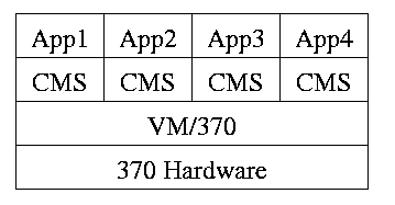
Use a ``hypervisor'' (beyond supervisor, i.e. beyond a normal OS) to
switch between multiple Operating Systems. Made popular by
IBM's VM/CMS
-
Each App/CMS runs on a virtual 370.
-
CMS is a single user OS.
-
A system call in an App traps to the corresponding CMS.
-
CMS believes it is running on the machine so issues I/O.
instructions but ...
-
... I/O instructions in CMS trap to VM/370.
-
This idea is still used.
A modern version (used to ``produce'' a multiprocessor from many
uniprocessors) is ``Cellular Disco'', ACM TOCS, Aug. 2000.
- Another modern usage is JVM the ``Java Virtual Machine''.
1.7.4: Exokernels
Similar to VM/CMS but the virtual machines have disjoint resources
(e.g., distinct disk blocks) so less remapping is needed.
1.7.5: Client Server
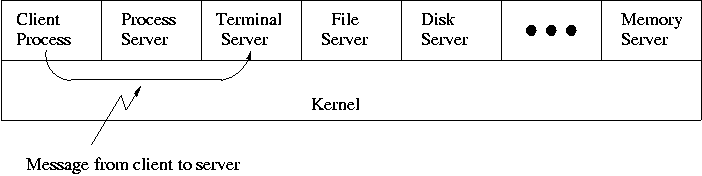
When implemented on one computer, a client server OS is using the
microkernel approach in which the microkernel just supplies
interprocess communication and the main OS functions are provided by a
number of separate processes.
This does have advantages. For example an error in the file server
cannot corrupt memory in the process server. This makes errors easier
to track down.
But it does mean that when a (real) user process makes a system call
there are more processes switches. These are
not free.
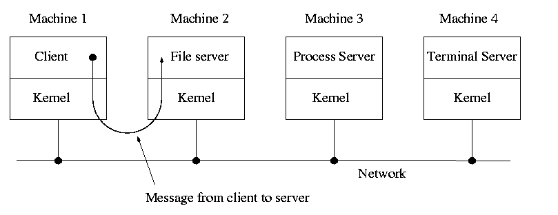
A distributed system can be thought of as an extension of the
client server concept where the servers are remote.
Homework: 23
Chapter 2: Process and Thread Management
Tanenbaum's chapter title is ``Processes and Threads''. I prefer to
add the word
management. The subject matter is processes, threads, scheduling,
interrupt handling, and IPC (InterProcess Communication--and
Coordination).
2.1: Processes
Definition: A process is a program
in execution.
- We are assuming a multiprogramming OS that
can switch from one process to another.
- Sometimes this is
called pseudoparallelism since one has the illusion of a
parallel processor.
- The other possibility is real
parallelism in which two or more processes are actually running
at once because the computer system is a parallel processor, i.e., has
more than one processor.
- We do not study real parallelism (parallel
processing, distributed systems, multiprocessors, etc) in this course.
2.1.1: The Process Model
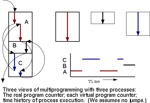
Even though in actuality there are many processes running at once, the
OS gives each process the illusion that it is running alone.
Virtual time and virtual memory are examples of abstractions
provided by the operating system to the user processes so that the
latter ``sees'' a more pleasant virtual machine than actually exists.
2.1.2: Process Creation
From the users or external viewpoint there are several mechanisms
for creating a process.
- System initialization, including daemon processes.
- Execution of a process creation system call by a running process.
- A user request to create a new process.
- Initiation of a batch job.
But looked at internally, from the system's viewpoint, the second
method dominates. Indeed in unix only one process is created at
system initialization (the process is called init); all the
others are children of this first process.
Why have init? That is why not have all processes created via
method 2?
Ans: Because without init there would be no running process to create
any others.
2.1.3: Process Termination
Again from the outside there appear to be several termination
mechanism.
- Normal exit (voluntary).
- Error exit (voluntary).
- Fatal error (involuntary).
- Killed by another process (involuntary).
And again, internally the situation is simpler. In Unix
terminology, there are two system calls kill and
exit that are used. Kill (poorly named in my view) sends a
signal to another process. If this signal is not caught (via the
signal system call) the process is terminated. There
is also an ``uncatchable'' signal. Exit is used for self termination
and can indicate success or failure.
2.1.4: Process Hierarchies
Modern general purpose operating systems permit a user to create and
destroy processes.
- In unix this is done by the fork
system call, which creates a child process, and the
exit system call, which terminates the current
process.
- After a fork both parent and child keep running (indeed they
have the same program text) and each can fork off other
processes.
- A process tree results. The root of the tree is a special
process created by the OS during startup.
- A process can choose to wait for children to terminate.
For example, if C issued a wait() system call it would block until G
finished.
Old or primitive operating system like
MS-DOS are not multiprogrammed, so when one process starts another,
the first process is automatically blocked and waits until
the second is finished.
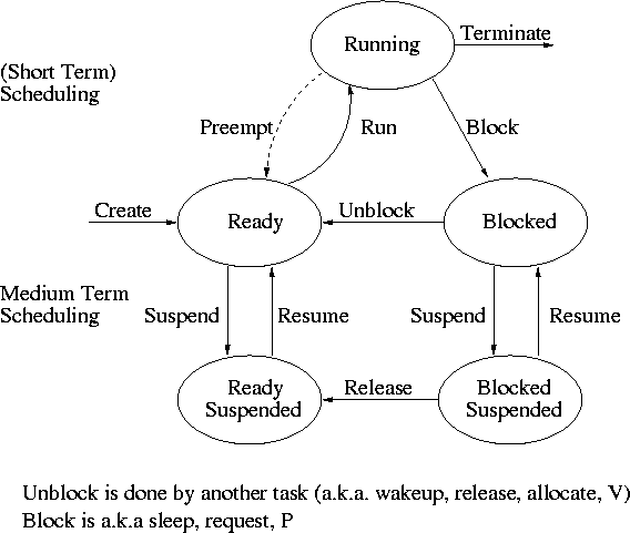
2.1.5: Process States and Transitions
The diagram on the right contains much information.
- Consider a running process P that issues an I/O request
- The process blocks
- At some later point, a disk interrupt occurs and the driver
detects that P's request is satisfied.
- P is unblocked, i.e. is moved from blocked to ready
- At some later time the operating system looks for a ready job
to run and picks P.
- A preemptive scheduler has the dotted line preempt;
A non-preemptive scheduler doesn't.
- The number of processes changes only for two arcs: create and
terminate.
- Suspend and resume are medium term scheduling
- Done on a longer time scale.
- Involves memory management as well.
- Sometimes called two level scheduling.
================ Start Lecture #4 ================
Remark:
Homework solutions will be posted (probably tomorrow).
In fact homework #1 solution is already there.
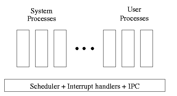
One can organize an OS around the scheduler.
- Write a minimal ``kernel'' consisting of the scheduler, interrupt
handlers, and IPC (interprocess communication).
- The rest of the OS consists of kernel processes (e.g. memory,
filesystem) that act as servers for the user processes (which of
course act as clients.
- The system processes also act as clients (of other system processes).
- The above is called the client-server model and is one Tanenbaum likes.
His ``Minix'' operating system works this way.
- Indeed, there was reason to believe that the client-server model
would dominate OS design.
But that hasn't happened.
- Such an OS is sometimes called server based.
- Systems like traditional unix or linux would then be
called self-service since the user process serves itself.
- That is, the user process switches to kernel mode and performs
the system call.
- To repeat: the same process changes back and forth from/to
user<-->system mode and services itself.
2.1.6: Implementation of Processes
The OS organizes the data about each process in a table naturally
called the process table.
Each entry in this table is called a
process table entry (PTE) or
process control block.
- One entry per process.
- The central data structure for process management.
- A process state transition (e.g., moving from blocked to ready) is
reflected by a change in the value of one or more
fields in the PTE.
- We have converted an active entity (process) into a data structure
(PTE). Finkel calls this the level principle ``an active
entity becomes a data structure when looked at from a lower level''.
- The PTE contains a great deal of information about the process.
For example,
- Saved value of registers when process not running
- Program counter (i.e., the address of the next instruction)
- Stack pointer
- CPU time used
- Process id (PID)
- Process id of parent (PPID)
- User id (uid and euid)
- Group id (gid and egid)
- Pointer to text segment (memory for the program text)
- Pointer to data segment
- Pointer to stack segment
- UMASK (default permissions for new files)
- Current working directory
- Many others
An aside on Interrupts (will be done again
here)
In a well defined location in memory (specified by the hardware) the
OS stores an interrupt vector, which contains the
address of the (first level) interrupt handler.
-
Tanenbaum calls the interrupt handler the interrupt service routine.
-
Actually one can have different priorities of interrupts and the
interrupt vector contains one pointer for each level. This is why it is
called a vector.
Assume a process P is running and a disk interrupt occurs for the
completion of a disk read previously issued by process Q, which is
currently blocked.
Note that disk interrupts are unlikely to be for the currently running
process (because the process that initiated the disk access is likely
blocked).
- The hardware saves the program counter and some other registers
(or switches to using another set of registers, the exact mechanism is
machine dependent).
- Hardware loads new program counter from the interrupt vector.
- Loading the program counter causes a jump.
- Steps 1 and 2 are similar to a procedure call.
But the interrupt is asynchronous.
- As with a trap (poof), the interrupt automatically switches
the system into privileged mode.
- Assembly language routine saves registers.
- Assembly routine sets up new stack.
- These last two steps can be called setting up the C environment.
- Assembly routine calls C procedure (Tanenbaum forgot this one).
- C procedure does the real work.
- Determines what caused the interrupt (in this case a disk
completed an I/O)
- How does it figure out the cause?
- Which priority interrupt was activated.
- The controller can write data in memory before the
interrupt
- The OS can read registers in the controller
- Mark process Q as ready to run.
- That is move Q to the ready list (note that again
we are viewing Q as a data structure).
- The state of Q is now ready (it was blocked before).
- The code that Q needs to run initially is likely to be OS
code. For example, Q probably needs to copy the data just
read from a kernel buffer into user space.
- Now we have at least two processes ready to run: P and Q
- The scheduler decides which process to run (P or Q or
something else). Lets assume that the decision is to run P.
- The C procedure (that did the real work in the interrupt
processing) continues and returns to the assembly code.
- Assembly language restores P's state (e.g., registers) and starts
P at the point it was when the interrupt occurred.
2.2: Threads
| Per process items | Per thread items
|
|---|
| Address space | Program counter
|
| Global variables | Machine registers
|
| Open files | Stack
|
| Child processes
|
| Pending alarms
|
| Signals and signal handlers
|
| Accounting information
|
The idea is to have separate threads of control (hence the name)
running in the same address space.
An address space is a memory management concept.
For now think of an address space as the memory in which a process
runs and the mapping from the virtual addresses (addresses in the
program) to the physical addresses (addresses in the machine).
Each thread is somewhat like a
process (e.g., it is scheduled to run) but contains less state
(e.g., the address space belongs to the process in which the thread runs.
2.2.1: The Thread Model
A process contains a number of resources such as address space,
open files, accounting information, etc. In addition to these
resources, a process has a thread of control, e.g., program counter,
register contents, stack. The idea of threads is to permit multiple
threads of control to execute within one process. This is often
called multithreading and threads are often called
lightweight processes. Because threads in the same
process share so much state, switching between them is much less
expensive than switching between separate processes.
Individual threads within the same process are not completely
independent. For example there is no memory protection between them.
This is typically not a security problem as the threads are
cooperating and all are from the same user (indeed the same process).
However, the shared resources do make debugging harder. For example
one thread can easily overwrite data needed by another and if one thread
closes a file other threads can't read from it.
2.2.2: Thread Usage
Often, when a process A is blocked (say for I/O) there is still
computation that can be done. Another process B can't do this
computation since it doesn't have access to the A's memory. But two
threads in the same process do share memory so there is no problem.
An important modern example is a multithreaded web server. Each thread is
responding to a single WWW connection. While one thread is blocked on
I/O, another thread can be processing another WWW connection. Why not
use separate processes, i.e., what is the shared memory?
Ans: The cache of frequently referenced pages.
A common organization is to have a dispatcher thread that fields
requests and then passes this request on to an idle thread.
Another example is a producer-consumer problem
(c.f. below)
in which we have 3 threads in a pipeline.
One reads data, the second processes the data read, and the third
outputs the processed data. Again, while one thread is blocked the
others can execute.
Homework: 9.
2.2.3: Implementing threads in user space
Write a (threads) library that acts as a mini-scheduler and
implements thread_create, thread_exit,
thread_wait, thread_yield, etc. The central data
structure maintained and used by this library is the thread
table, the analogue of the process table in the operating system
itself.
Advantages
- Requires no OS modification.
- Very fast since no context switching.
- Can customize the scheduler for each application.
Disadvantages
- Re-doing the effort of writing a scheduler.
- Blocking system calls can't be executed directly since that would block
the entire process.
- Similarly a page fault would block the entire process.
- A thread with infinite loop prevents all other threads in this
process from running.
2.2.4: Implementing Threads in the Kernel
Move the thread operations into the operating system itself. This
naturally requires that the operating system itself be (significantly)
modified and is thus not a trivial undertaking.
- Thread-create and friends are now system calls and hence much
slower than with user-mode threads.
They are, however, still much faster than creating/switching/etc
processes since there is so much shared state that does not need
to be recreated.
- During this past summer (2002), Ingo Molnar has been speeding
up the linux kernel thread performance with the goal that a pure kernel
level thread system will achieve (nearly) the speed of a user mode
system.
Benchmarking has begun; results should be available in a few months.
- A thread that blocks causes no particular problem. The kernel can
run another thread from this process or can run another process.
- Similarly a page fault, or infinite loop in one thread does not
automatically block the other threads in the process.
2.2.5: Hybrid Implementations
One can write a (user-level) thread library even if the kernel also
has threads. This is sometimes called the M:N model since M user mode threads
run on each of N kernel threads.
Then each kernel thread can switch between user level
threads. Thus switching between user-level threads within one kernel
thread is very fast (no context switch) and we maintain the advantage
that a blocking system call or page fault does not block the entire
multi-threaded application.
2.2.6: Scheduler Activations
Skipped
2.2.7: Popup Threads
The idea is to automatically issue a create thread system call upon
message arrival. (The alternative is to have a thread or process
blocked on a receive system call.)
If implemented well the latency between message arrival and thread
execution can be very small since the new thread does not have state
to restore.
Making Single-threaded Code Multithreaded
Definitely NOT for the faint of heart.
- There often is state that should not be shared. A well-cite
example is the unix errno variable that contains the error
number (zero means no error) of the error encountered by the last
system call. Errno is hardly elegant (even in normal,
single-threaded, applications), but its use is widespread.
If multiple threads issue faulty system calls the errno value of the
second overwrites the first and thus the first errno value may be lost.
- Much existing code, including many libraries, are not
re-entrant.
- What should be done with a signal sent to a process. Does it go
to all or one thread?
- How should stack growth be managed. Normally the kernel grows the
(single) stack automatically when needed. What if there are
multiple stacks?
2.3: Interprocess Communication (IPC) and Coordination/Synchronization
2.3.1: Race Conditions
A race condition occurs when two processes can
interact and the outcome depends on the order in which the processes
execute.
Imagine two processes both accessing x, which is initially 10.
- One process is to execute x <-- x+1
- The other is to execute x <-- x-1
- When both are finished x should be 10
- But we might get 9 and might get 11!
- Show how this can happen (x <-- x+1 is not atomic)
- Tanenbaum shows how this can lead to disaster for a printer
spooler
Homework: 18.
2.3.2: Critical sections
We must prevent interleaving sections of code that need to be atomic with
respect to each other. That is, the conflicting sections need
mutual exclusion. If process A is executing its
critical section, it excludes process B from executing its critical
section. Conversely if process B is executing is critical section, it
excludes process A from executing its critical section.
Requirements for a critical section implementation.
- No two processes may be simultaneously inside their critical
section.
- No assumption may be made about the speeds or the number of CPUs.
- No process outside its critical section may block other processes.
- No process should have to wait forever to enter its critical
section.
- I do NOT make this last requirement.
- I just require that the system as a whole make progress (so not
all processes are blocked).
- I refer to solutions that do not satisfy Tanenbaum's last
condition as unfair, but nonetheless correct, solutions.
- Stronger fairness conditions have also been defined.
2.3.3 Mutual exclusion with busy waiting
The operating system can choose not to preempt itself.
That is, we do not preempt system processes (if the OS is client server) or
processes running in system mode (if the OS is self service).
Forbidding preemption for system processes would prevent the problem
above where x<--x+1 not being atomic crashed the printer spooler if
the spooler is part of the OS.
But simply forbidding preemption while in system mode is not sufficient.
- Does not work for user-mode programs. So the Unix print spooler would
not be helped.
- Does not prevent conflicts between the main line OS and interrupt
handlers.
- This conflict could be prevented by disabling
interrupts while the main
line is in its critical section.
- Indeed, disabling (a.k.a. temporarily preventing) interrupts
is often done for exactly this reason.
- Do not want to block interrupts for too long or the system
will seem unresponsive.
- Does not work if the system has several processors.
- Both main lines can conflict.
- One processor cannot block interrupts on the other.
Software solutions for two processes
Initially P1wants=P2wants=false

Code for P1                             Code for P2

Loop forever {                          Loop forever {
    P1wants <-- true         ENTRY          P2wants <-- true
    while (P2wants) {}       ENTRY          while (P1wants) {}
    critical-section                        critical-section
    P1wants <-- false        EXIT           P2wants <-- false
    non-critical-section }                  non-critical-section }
Explain why this works.
But it is wrong! Why?
Let's try again. The trouble was that setting want before the
loop permitted us to get stuck. We had them in the wrong order!
Initially P1wants=P2wants=false

Code for P1                             Code for P2

Loop forever {                          Loop forever {
    while (P2wants) {}       ENTRY          while (P1wants) {}
    P1wants <-- true         ENTRY          P2wants <-- true
    critical-section                        critical-section
    P1wants <-- false        EXIT           P2wants <-- false
    non-critical-section }                  non-critical-section }
Explain why this works.
But it is wrong again! Why?
So let's be polite and really take turns. None of this wanting stuff.
Initially turn=1

Code for P1                      Code for P2

Loop forever {                   Loop forever {
    while (turn = 2) {}              while (turn = 1) {}
    critical-section                 critical-section
    turn <-- 2                       turn <-- 1
    non-critical-section }           non-critical-section }
This one forces alternation, so is not general enough. Specifically,
it does not satisfy condition three, which requires that no process in
its non-critical section can stop another process from entering its
critical section. With alternation, if one process is in its
non-critical section (NCS) then the other can enter the CS once but
not again.
In fact, it took years (way back when) to find a correct solution.
Many earlier ``solutions'' were found and several were published, but
all were wrong.
The first correct solution was found by a mathematician named Dekker,
who combined the ideas of turn and wants.
The basic idea is that you take turns when there is contention, but
when there is no contention, the requesting process can enter.
It is very clever, but I am skipping it (I cover it when I teach
distributed operating systems in V22.0480 or G22.2251).
Subsequently, algorithms with better fairness properties were found
(e.g., no task has to wait for another task to enter the CS twice).
What follows is Peterson's solution, which also combines turn and
wants to force alternation only when there is contention.
When Peterson's solution was published, it was a
surprise to see such a simple soluntion. In fact Peterson gave a
solution for any number of processes. A proof that the algorithm
satisfies our properties (including a strong fairness condition)
for any number of processes can
be found in Operating Systems Review Jan 1990, pp. 18-22.
Initially P1wants=P2wants=false  and  turn=1

Code for P1                        Code for P2

Loop forever {                     Loop forever {
    P1wants <-- true                   P2wants <-- true
    turn <-- 2                         turn <-- 1
    while (P2wants and turn=2) {}      while (P1wants and turn=1) {}
    critical-section                   critical-section
    P1wants <-- false                  P2wants <-- false
    non-critical-section               non-critical-section
================ Start Lecture #5 ================
Hardware assist (test and set)
TAS(b), where b is a binary variable,
ATOMICALLY sets b<--true and returns the OLD value of b.
Of course it would be silly to return the new value of b since we know
the new value is true.
The word atomically means that the two actions
performed by TAS(x) (testing, i.e., returning the old value of x and
setting , i.e., assigning true to x) are inseparable.
Specifically it is not possible for two concurrent TAS(x)
operations to both return false (unless there is also another
concurrent statement that sets x to false).
With TAS available implementing a critical section for any number
of processes is trivial.
loop forever {
    while (TAS(s)) {}   ENTRY
    CS
    s<--false           EXIT
    NCS
2.3.4: Sleep and Wakeup
Remark:
Tanenbaum does both busy waiting (as above)
and blocking (process switching) solutions.
We will only do busy waiting, which is easier.
Sleep and Wakeup are the simplest blocking primitives.
Sleep voluntarily blocks the process and wakeup unblocks a sleeping
process.
We will not cover these.
Homework:
Explain the difference between busy waiting and blocking.
2.3.5: Semaphores
Remark:
Tannenbaum use the term semaphore only
for blocking solutions.
I will use the term for our busy waiting solutions.
Others call our solutions spin locks.
P and V and Semaphores
The entry code is often called P and the exit code V.
Thus the critical section problem is to write P and V so that
loop forever
    P
    critical-section
    V
    non-critical-section
satisfies
- Mutual exclusion.
- No speed assumptions.
- No blocking by processes in NCS.
- Forward progress (my weakened version of Tanenbaum's last condition).
Note that I use indenting carefully and hence do not need (and
sometimes omit) the braces {} used in languages like C or java.
A binary semaphore abstracts the TAS solution we gave
for the critical section problem.
The above code is not real, i.e., it is not an
implementation of P. It is, instead, a definition of the effect P is
to have.
To repeat: for any number of processes, the critical section problem can be
solved by
loop forever
    P(S)
    CS
    V(S)
    NCS
The only specific solution we have seen for an arbitrary number of
processes is the one just above with P(S) implemented via
test and set.
Remark: Peterson's solution requires each process to
know its processor number. The TAS soluton does not.
Moreover the definition of P and V does not permit use of the
processor number.
Thus, strictly speaking Peterson did not provide an implementation of
P and V.
He did solve the critical section problem.
To solve other coordination problems we want to extend binary
semaphores.
- With binary semaphores, two consecutive Vs do not permit two
subsequent Ps to succeed (the gate cannot be doubly opened).
- We might want to limit the number of processes in the section to
3 or 4, not always just 1.
Both of the shortcomings can be overcome by not restricting ourselves
to a binary variable, but instead define a
generalized or counting semaphore.
- A counting semaphore S takes on non-negative integer values
- Two operations are supported
- P(S) is
    while (S=0) {}
    S--
where finding S>0 and decrementing S is atomic
- That is, wait until the gate is open (positive), then run through and
atomically close the gate one unit
- Another way to describe this atomicity is to say that it is not
possible for the decrement to occur when S=0 and it is also not
possible for two processes executing P(S)
simultaneously to both see the same necessarily (positive) value of S
unless a V(S) is also simultaneous.
- V(S) is simply S++
These counting semaphores can solve what I call the
semi-critical-section problem, where you premit up to k
processes in the section. When k=1 we have the original
critical-section problem.
initially S=k

loop forever
    P(S)
    SCS   <== semi-critical-section
    V(S)
    NCS
Producer-consumer problem
- Two classes of processes
- Producers, which produce times and insert them into a buffer.
- Consumers, which remove items and consume them.
- What if the producer encounters a full buffer?
Answer: It waits for the buffer to become non-full.
- What if the consumer encounters an empty buffer?
Answer: It waits for the buffer to become non-empty.
- Also called the bounded buffer problem.
- Another example of active entities being replaced by a data
structure when viewed at a lower level (Finkel's level principle).
Initially e=k, f=0 (counting semaphore); b=open (binary semaphore)

Producer                         Consumer

loop forever                     loop forever
    produce-item                     P(f)
    P(e)                             P(b); take item from buf; V(b)
    P(b); add item to buf; V(b)      V(e)
    V(f)                             consume-item
- k is the size of the buffer
- e represents the number of empty buffer slots
- f represents the number of full buffer slots
- We assume the buffer itself is only serially accessible. That is,
only one operation at a time.
- This explains the P(b) V(b) around buffer operations
- I use ; and put three statements on one line to suggest that
a buffer insertion or removal is viewed as one atomic operation.
- Of course this writing style is only a convention, the
enforcement of atomicity is done by the P/V.
- The P(e), V(f) motif is used to force ``bounded alternation''. If k=1
it gives strict alternation.
2.3.6: Mutexes
Remark:
Whereas we use the term semaphore to mean binary semaphore and
explicitly say generalized or counting semaphore for the positive
integer version, Tanenbaum uses semaphore for the positive integer
solution and mutex for the binary version.
Also, as indicated above, for Tanenbaum semaphore/mutex implies a
blocking primitive; whereas I use binary/counting semaphore for both
busy-waiting and blocking implementations. Finally, remember that in
this course we are studying only busy-waiting solutions.
My Terminology
| | Busy wait | block/switch
|
|---|
| critical | (binary) semaphore | (binary) semaphore
|
| semi-critical | counting semaphore | counting semaphore
|
Tanenbaum's Terminology
| | Busy wait | block/switch
|
|---|
| critical | enter/leave region | mutex
|
| semi-critical | no name | semaphore
|
2.3.7: Monitors
Skipped.
2.3..8: Message Passing
Skipped.
You can find some information on barriers in my
lecture notes for a follow-on course
(see in particular lecture #16).
2.4: Classical IPC Problems
2.4.1: The Dining Philosophers Problem
A classical problem from Dijkstra
- 5 philosophers sitting at a round table
- Each has a plate of spaghetti
- There is a fork between each two
- Need two forks to eat
What algorithm do you use for access to the shared resource (the
forks)?
- The obvious solution (pick up right; pick up left) deadlocks.
- Big lock around everything serializes.
- Good code in the book.
The purpose of mentioning the Dining Philosophers problem without giving
the solution is to give a feel of what coordination problems are like.
The book gives others as well. We are skipping these (again this
material would be covered in a sequel course). If you are interested
look, for example,
here.
Homework: 31 and 32 (these have short answers but are
not easy). Note that the problem refers to fig. 2-20, which is
incorrect. It should be fig 2-33, as noticed by Liang Chen.
2.4.2: The Readers and Writers Problem
- Two classes of processes.
- Readers, which can work concurrently.
- Writers, which need exclusive access.
- Must prevent 2 writers from being concurrent.
- Must prevent a reader and a writer from being concurrent.
- Must permit readers to be concurrent when no writer is active.
- Perhaps want fairness (e.g., freedom from starvation).
- Variants
- Writer-priority readers/writers.
- Reader-priority readers/writers.
Quite useful in multiprocessor operating systems and database systems.
The ``easy way
out'' is to treat all processes as writers in which case the problem
reduces to mutual exclusion (P and V). The disadvantage of the easy
way out is that you give up reader concurrency.
Again for more information see the web page referenced above.
2.4.3: The Sleeping Barber Problem
Skipped.
2.5: Process Scheduling
Scheduling processes on the processor is often called ``process
scheduling'' or simply ``scheduling''.
The objectives of a good scheduling policy include
- Fairness.
- Efficiency.
- Low response time (important for interactive jobs).
- Low turnaround time (important for batch jobs).
- High throughput [the above are from Tanenbaum].
- More ``important'' processes are favored.
- Interactive processes are favored.
- Repeatability. Dartmouth (DTSS) ``wasted cycles'' and limited
logins for repeatability.
- Fair across projects.
- ``Cheating'' in unix by using multiple processes.
- TOPS-10.
- Fair share research project.
- Degrade gracefully under load.
Recall the basic diagram describing process states
For now we are discussing short-term scheduling, i.e., the arcs
connecting running <--> ready.
Medium term scheduling is discussed later.
Preemption
It is important to distinguish preemptive from non-preemptive
scheduling algorithms.
- Preemption means the operating system moves a process from running
to ready without the process requesting it.
- Without preemption, the system implements ``run to completion (or
yield or block)''.
- The ``preempt'' arc in the diagram.
- We do not consider yield (a solid arrow from running to ready).
- Preemption needs a clock interrupt (or equivalent).
- Preemption is needed to guarantee fairness.
- Found in all modern general purpose operating systems.
- Even non preemptive systems can be multiprogrammed (e.g., when processes
block for I/O).
================ Start Lecture #6 ================
Deadline scheduling
This is used for real time systems. The objective of the scheduler is
to find a schedule for all the tasks (there are a fixed set of tasks)
so that each meets its deadline. The run time of each task is known
in advance.
Actually it is more complicated.
- Periodic tasks
- What if we can't schedule all task so that each meets its deadline
(i.e., what should be the penalty function)?
- What if the run-time is not constant but has a known probability
distribution?
We do not cover deadline scheduling in this course.
The name game
There is an amazing inconsistency in naming the different
(short-term) scheduling algorithms. Over the years I have used
primarily 4 books: In chronological order they are Finkel, Deitel,
Silberschatz, and Tanenbaum. The table just below illustrates the
name game for these four books. After the table we discuss each
scheduling policy in turn.
Finkel  Deitel  Silbershatz Tanenbaum
-------------------------------------
FCFS    FIFO    FCFS        --    unnamed in tanenbaum
RR      RR      RR          RR
PS      **      PS          PS
SRR     **      SRR         **    not in tanenbaum
SPN     SJF     SJF         SJF
PSPN    SRT     PSJF/SRTF   --    unnamed in tanenbaum
HPRN    HRN     **          **    not in tanenbaum
**      **      MLQ         **    only in silbershatz
FB      MLFQ    MLFQ        MQ
Remark: For an alternate organization of the
scheduling algorithms (due to Eric Freudenthal and presented by him
Fall 2002) click here.
First Come First Served (FCFS, FIFO, FCFS, --)
If the OS ``doesn't'' schedule, it still needs to store the PTEs
somewhere. If it is a queue you get FCFS. If it is a stack
(strange), you get LCFS. Perhaps you could get some sort of random
policy as well.
- Only FCFS is considered.
- The simplist scheduling policy.
- Non-preemptive.
Round Robin (RR, RR, RR, RR)
- An important preemptive policy.
- Essentially the preemptive version of FCFS.
- The key parameter is the quantum size q.
- When a process is put into the running state a timer is set to q.
- If the timer goes off and the process is still running, the OS
preempts the process.
- This process is moved to the ready state (the
preempt arc in the diagram), where it is placed at the
rear of the ready list (a queue).
- The process at the front of the ready list is removed from
the ready list and run (i.e., moves to state running).
- When a process is created, it is placed at the rear of the ready list.
- As q gets large, RR approaches FCFS
- As q gets small, RR approaches PS (Processor Sharing, described next)
- What value of q should we choose?
- Trade-off
- Small q makes system more responsive.
- Large q makes system more efficient since less process switching.
Homework: 26, 35, 38.
Homework: Give an argument favoring a large
quantum; give an argument favoring a small quantum.
| Process | CPU Time | Creation Time |
|---|
| P1 | 20 | 0 |
| P2 | 3 | 3 |
| P3 | 2 | 5 |
Homework:
(Remind me to discuss this last one in class next time):
Consider the set of processes in the table below.
When does each process finish if RR scheduling is used with q=1, if
q=2, if q=3, if q=100. First assume (unrealistically) that context
switch time is zero. Then assume it is .1.
Each process performs no
I/O (i.e., no process ever blocks). All times are in milliseconds.
The CPU time is the total time required for the process (excluding any
context switch time). The creation
time is the time when the process is created. So P1 is created when
the problem begins and P3 is created 5 milliseconds later.
If two processes have equal priority (in RR this means if thy both
enter the ready state at the same cycle), we give priority (in RR this
means place first on the queue) to the process with the earliest
creation time.
If they also have the same creation time, then we give priority to the
process with the lower number.
Processor Sharing (PS, **, PS, PS)
Merge the ready and running states and permit all ready jobs to be run
at once. However, the processor slows down so that when n jobs are
running at once, each progresses at a speed 1/n as fast as it would if
it were running alone.
- Clearly impossible as stated due to the overhead of process
switching.
- Of theoretical interest (easy to analyze).
- Approximated by RR when the quantum is small. Make
sure you understand this last point. For example,
consider the last homework assignment (with zero context switch time)
and consider q=1, q=.1, q=.01, etc.
Homework: 34.
Variants of Round Robin
- State dependent RR
- Same as RR but q is varied dynamically depending on the state
of the system.
- Favor processes holding important resources.
- For example, non-swappable memory.
- Perhaps this should be considered medium term scheduling
since you probably do not recalculate q each time.
- External priorities: RR but a user can pay more and get
bigger q. That is one process can be given a higher priority than
another. But this is not an absolute priority: the lower priority
(i.e., less important) process does get to run, but not as much as the
higher priority process.
Priority Scheduling
Each job is assigned a priority (externally, perhaps by charging
more for higher priority) and the highest priority ready job is run.
- Similar to ``External priorities'' above
- If many processes have the highest priority, use RR among them.
- Can easily starve processes (see aging below for fix).
- Can have the priorities changed dynamically to favor processes
holding important resources (similar to state dependent RR).
- Many policies can be thought of as priority scheduling in
which we run the job with the highest priority (with different notions
of priority for different policies).
Priority aging
As a job is waiting, raise its priority so eventually it will have the
maximum priority.
- This prevents starvation (assuming all jobs terminate or the
policy is preemptive).
- There may be many processes with the maximum priority.
- If so, can use FIFO among those with max priority (risks
starvation if a job doesn't terminate) or can use RR.
- Can apply priority aging to many policies, in particular to priority
scheduling described above.
Selfish RR (SRR, **, SRR, **)

- Preemptive.
- Perhaps it should be called ``snobbish RR''.
- ``Accepted processes'' run RR.
- Accepted process have their priority increase at rate b>=0.
- A new process starts at priority 0; its priority increases at rate a>=0.
- A new process becomes an accepted process when its priority
reaches that of an accepted process (or when there are no accepted
processes).
- Once a process is accepted it remains accepted until it terminates.
- Note that at any time all accepted processes have same priority.
- If b>=a, get FCFS.
- If b=0, get RR.
- If a>b>0, it is interesting.
Shortest Job First (SPN, SJF, SJF, SJF)
Sort jobs by total execution time needed and run the shortest first.
- Nonpreemptive
- First consider a static situation where all jobs are available in
the beginning and we know how long each one takes to run.
For simplicity lets consider ``run-to-completion'', also called
``uniprogrammed'' (i.e., we don't even switch to another
process on I/O).
In this situation, uniprogrammed SJF has the shortest average
waiting time
- Assume you have a schedule with a long job right before a
short job.
- Consider swapping the two jobs.
- This decreases the wait for
the short by the length of the long job and increases the wait of the
long job by the length of the short job.
- This decreases the total waiting time for these two.
- Hence decreases the total waiting for all jobs and hence decreases
the average waiting time as well.
- Hence, whenever a long job is right before a short job, we can
swap them and decrease the average waiting time.
- Thus the lowest average waiting time occurs when there are no
short jobs right before long jobs.
- This is uniprogrammed SJF.
- In the more realistic case of true SJF where the scheduler
switches to a new process when the currently running process
blocks (say for I/O), we should call the policy shortest
next-CPU-burst first.
- The difficulty is predicting the future (i.e., knowing in advance
the time required for the job or next-CPU-burst).
- This is an example of priority scheduling.
Homework: 39, 40 (note that when he says RR with
each process getting its fair share, he means PS).
Preemptive Shortest Job First (PSPN, SRT, PSJF/SRTF, --)
Preemptive version of above
- Permit a process that enters the ready list to preempt the running
process if the time for the new process (or for its next burst) is
less than the remaining time for the running process (or for
its current burst).
- It will never happen that a process in the ready list
will require less time than the remaining time for the currently
running process. Why?
Ans: When the process joined the ready list it would have started
running if the current process had more time remaining. Since
that didn't happen the current job had less time remaining and now
it has even less.
- Can starve processs that require a long burst.
- This is fixed by the standard technique.
- What is that technique?
Ans: Priority aging.
- Another example of priority scheduling.
Highest Penalty Ratio Next (HPRN, HRN, **, **)
Run the process that has been ``hurt'' the most.
- For each process, let r = T/t; where T is the wall clock time this
process has been in system and t is the running time of the process to
date.
- If r=5, that means the job has been running 1/5 of the time it has been
in the system.
- We call r the penalty ratio and run the process having
the highest r value.
- HPRN is normally defined to be non-preemptive (i.e., the system
only checks r when a burst ends), but there is an preemptive analogue
- Do not worry about a process that just enters the system (its
ratio is undefined)
- When putting process into the run state compute the time at
which it will no longer have the highest ratio and set a timer.
- When a process is moved into the ready state, compute its ratio
and preempt if needed.
- HRN stands for highest response ratio next and means the same thing.
- This policy is yet another example of priority scheduling
Multilevel Queues (**, **, MLQ, **)
Put different classes of processs in different queues
- Processs do not move from one queue to another.
- Can have different policies on the different queues.
For example, might have a background (batch) queue that is FCFS and one or
more foreground queues that are RR.
- Must also have a policy among the queues.
For example, might have two queues, foreground and background, and give
the first absolute priority over the second
- Might apply aging to prevent background starvation.
- But might not, i.e., no guarantee of service for background
processes. View a background process as a ``cycle soaker''.
- Might have 3 queues, foreground, background, cycle soaker
Multilevel Feedback Queues (FB, MFQ, MLFBQ, MQ)
Many queues and processs move from queue to queue in an attempt to
dynamically separate ``batch-like'' from interactive processs so that
we can favor the latter.
- Run processs from the highest priority nonempty queue in a RR manner.
- When a process uses its full quanta (looks a like batch process),
move it to a lower priority queue.
- When a process doesn't use a full quanta (looks like an interactive
process), move it to a higher priority queue.
- A long process with frequent (perhaps spurious) I/O will remain
in the upper queues.
- Might have the bottom queue FCFS.
- Many variants
For example, might let process stay in top queue 1 quantum, next queue 2
quanta, next queue 4 quanta (i.e. return a process to the rear of the
same queue it was in if the quantum expires).
Theoretical Issues
Considerable theory has been developed.
- NP completeness results abound.
- Much work in queuing theory to predict performance.
- Not covered in this course.
Medium-Term Scheduling
In addition to the short-term scheduling we have discussed, we add
medium-term scheduling in which
decisions are made at a coarser time scale.
- Called memory scheduling by Tanenbaum (part of three level scheduling).
- Suspend (swap out) some process if memory is over-committed.
- Criteria for choosing a victim.
- How long since previously suspended.
- How much CPU time used recently.
- How much memory does it use.
- External priority (pay more, get swapped out less).
- We will discuss medium term scheduling again when we study memory
management.
Long Term Scheduling
- ``Job scheduling''. Decide when to start jobs, i.e., do not
necessarily start them when submitted.
- Force user to log out and/or block logins if over-committed.
- CTSS (an early time sharing system at MIT) did this to insure
decent interactive response time.
- Unix does this if out of processes (i.e., out of PTEs).
- ``LEM jobs during the day'' (Grumman).
- Called admission scheduling by Tanenbaum (part of three level scheduling).
- Many supercomputer sites.
2.5.4: Scheduling in Real Time Systems
Skipped
2.5.5: Policy versus Mechanism
Skipped.
2.5.6: Thread Scheduling
Skipped.
Research on Processes and Threads
Skipped.
Notes on lab (scheduling)
- If several processes are waiting on I/O, you may assume
noninterference. For example, assume that on cycle 100 process A
flips a coin and decides its wait is 6 units (i.e., during cycles
101-106 A will be blocked. Assume B begins running at cycle 101 for a
burst of 1 cycle. So during 101
process B flips a coin and decides its wait is 3 units. You do NOT
alter process A. That is, Process A will become ready after
cycle 106 (100+6) so enters the ready list cycle 107 and process B
becomes ready after cycle 104 (101+3) and enters ready list cycle
105.
- For processor sharing (PS), which is part of the extra credit:
PS (processor sharing). Every cycle you see how many jobs are
ready (or running). Say there are 7. Then during this cycle (an exception
will be described below) each process gets 1/7 of a cycle.
EXCEPTION: Assume there are exactly 2 ready jobs, one needs 1/3 cycle
and one needs 1/2 cycle. The process needing only 1/3 gets only 1/3,
i.e. it is finished after 2/3 cycle. So the other process gets 1/3
cycle during the first 2/3 cycle and then starts to get all the CPU.
Hence it finishes after 2/3 + 1/6 = 5/6 cycle. The last 1/6 cycle is
not used by any process.
End of Notes
Chapter 3: Deadlocks
A deadlock occurs when every member of a set of
processes is waiting for an event that can only be caused
by a member of the set.
Often the event waited for is the release of a resource.
In the automotive world deadlocks are called gridlocks.
- The processes are the cars.
- The resources are the spaces occupied by the cars
Reward: One point extra credit on the final exam
for anyone who brings a real (e.g., newspaper) picture of an
automotive deadlock. You must bring the clipping to the final and it
must be in good condition. Hand it in with your exam paper.
Note that it must really be a gridlock, i.e., motion is not possible
without breaking the traffic rules. A huge traffic jam is not
sufficient.
For a computer science example consider two processes A and B that
each want to print a file currently on tape.
- A has obtained ownership of the printer and will release it after
printing one file.
- B has obtained ownership of the tape drive and will release it after
reading one file.
- A tries to get ownership of the tape drive, but is told to wait
for B to release it.
- B tries to get ownership of the printer, but is told to wait for
A to release the printer.
Bingo: deadlock!
================ Start Lecture #7 ================
3.1: Resources:
The resource is the object granted to a process.
3.1.1: Preemptable and Nonpreemptable Resourses
- Resources come in two types
- Preemptable, meaning that the resource can be
taken away from its current owner (and given back later). An
example is memory.
- Non-preemptable, meaning that the resource
cannot be taken away. An example is a printer.
- The interesting issues arise with non-preemptable resources so
those are the ones we study.
- Life history of a resource is a sequence of
- Request
- Allocate
- Use
- Release
- Processes make requests, use the resourse, and release the
resourse. The allocate decisions are made by the system and we will
study policies used to make these decisions.
3.1.2: Resourse Acquisition
Simple example of the trouble you can get into.
- Two resources and two processes.
- Each process wants both resources.
- Use a semaphore for each. Call them S and T.
- If both processes execute P(S); P(T); --- V(T); V(S)
all is well.
- But if one executes instead P(T); P(S); -- V(S); V(T)
disaster! This was the printer/tape example just above.
Recall from the semaphore/critical-section treatment last
chapter, that it is easy to cause trouble if a process dies or stays
forever inside its critical section.
Similarly, we assume that no process maintains a resource forever.
It may obtain the resource an unbounded number of times (i.e. it can
have a loop forever with a resource request inside), but each time it
gets the resource, it must release it eventually.
3.2: Introduction to Deadlocks
To repeat: A deadlock occurs when a every member of a set of
processes is waiting for an event that can only be caused
by a member of the set.
Often the event waited for is the release of
a resource.
3.2.1: (Necessary) Conditions for Deadlock
The following four conditions (Coffman; Havender) are
necessary but not sufficient for deadlock. Repeat:
They are not sufficient.
- Mutual exclusion: A resource can be assigned to at most one
process at a time (no sharing).
- Hold and wait: A processing holding a resource is permitted to
request another.
- No preemption: A process must release its resources; they cannot
be taken away.
- Circular wait: There must be a chain of processes such that each
member of the chain is waiting for a resource held by the next member
of the chain.
The first three are characteristics of the system and resources.
For a given system fixed set of resource they are either true or
false, i.e., they don't change with time.
The truth or falsehood of the last condition does indeed change with
time as the resources are requested/allocated/released.

3.2.2: Deadlock Modeling
On the right is the Resource Allocation Graph,
also called the Reusable Resource Graph.
- The processes are circles.
- The resources are squares.
- An arc (directed line) from a process P to a resource R signifies
that process P has requested (but not yet been allocated) resource R.
- An arc from a resource R to a process P indicates that process P
has been allocated resource R.
Homework: 5.
Consider two concurrent processes P1 and P2 whose programs are.
P1: request R1       P2: request R2
    request R2           request R1
    release R2           release R1
    release R1           release R2
On the board draw the resource allocation graph for various possible
executions of the processes, indicating when deadlock occurs and when
deadlock is no longer avoidable.
There are four strategies used for dealing with deadlocks.
- Ignore the problem
- Detect deadlocks and recover from them
- Avoid deadlocks by carefully deciding when to allocate resources.
- Prevent deadlocks by violating one of the 4 necessary conditions.
3.3: Ignoring the problem--The Ostrich Algorithm
The ``put your head in the sand approach''.
- If the likelihood of a deadlock is sufficiently small and the cost
of avoiding a deadlock is sufficiently high it might be better to
ignore the problem. For example if each PC deadlocks once per 100
years, the one reboot may be less painful that the restrictions needed
to prevent it.
- Clearly not a good philosophy for nuclear missile launchers.
- For embedded systems (e.g., missile launchers) the programs run
are fixed in advance so many of the questions Tanenbaum raises (such
as many processes wanting to fork at the same time) don't occur.
3.4: Detecting Deadlocks and Recovering From Them
3.4.1: Detecting Deadlocks with Single Unit Resources
Consider the case in which there is only one
instance of each resource.
- So a request can be satisfied by only one specific resource.
- In this case the 4 necessary conditions for
deadlock are also sufficient.
- Remember we are making an assumption (single unit resources) that
is often invalid. For example, many systems have several printers and
a request is given for ``a printer'' not a specific printer.
Similarly, one can have many tape drives.
- So the problem comes down to finding a directed cycle in the resource
allocation graph. Why?
Answer: Because the other three conditions are either satisfied by the
system we are studying or are not in which case deadlock is not a
question. That is, conditions 1,2,3 are conditions on the system in
general not on what is happening right now.
To find a directed cycle in a directed graph is not hard. The
algorithm is in the book. The idea is simple.
- For each node in the graph do a depth first traversal (hoping the
graph is a DAG (directed acyclic graph), building a list as you go
down the DAG.
- If you ever find the same node twice on your list, you have found
a directed cycle and the graph is not a DAG and deadlock exists among
the processes in your current list.
- If you never find the same node twice, the graph is a DAG and no
deadlock occurs.
- The searches are finite since the list size is bounded by the
number of nodes.
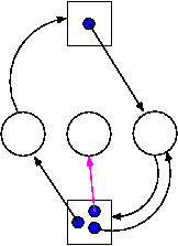
3.4.2: Detecting Deadlocks with Multiple Unit Resources
This is more difficult.
- The figure on the right shows a resource allocation graph with
multiple unit resources.
- Each unit is represented by a dot in the box.
- Request edges are drawn to the box since they represent a request
for any dot in the box.
- Allocation edges are drawn from the dot to represent that this
unit of the resource has been assigned (but all units of a resource
are equivalent and the choice of which one to assign is arbitrary).
- Note that there is a directed cycle in black, but there is no
deadlock. Indeed the middle process might finish, erasing the magenta
arc and permitting the blue dot to satisfy the rightmost process.
- The book gives an algorithm for detecting deadlocks in this more
general setting. The idea is as follows.
- look for a process that might be able to terminate (i.e., all
its request arcs can be satisfied).
- If one is found pretend that it does terminate (erase all its
arcs), and repeat step 1.
- If any processes remain, they are deadlocked.
- We will soon do in detail an algorithm (the Banker's algorithm) that
has some of this flavor.
3.4.3: Recovery from deadlock
Preemption
Perhaps you can temporarily preempt a resource from a process. Not
likely.
Rollback
Database (and other) systems take periodic checkpoints. If the
system does take checkpoints, one can roll back to a checkpoint
whenever a deadlock is detected. Somehow must guarantee forward
progress.
Kill processes
Can always be done but might be painful. For example some
processes have had effects that can't be simply undone. Print, launch
a missile, etc.
Remark:
We are doing 3.6 before 3.5 since 3.6 is easier.
3.6: Deadlock Prevention
Attack one of the coffman/havender conditions
3.6.1: Attacking Mutual Exclusion
Idea is to use spooling instead of mutual exclusion. Not
possible for many kinds of resources
3.6.2: Attacking Hold and Wait
Require each processes to request all resources at the beginning
of the run. This is often called One Shot.
3.6.3: Attacking No Preempt
Normally not possible.
3.6.4: Attacking Circular Wait
Establish a fixed ordering of the resources and require that they
be requested in this order. So if a process holds resources #34 and
#54, it can request only resources #55 and higher.
It is easy to see that a cycle is no longer possible.
Homework: 7.
3.5: Deadlock Avoidance
Let's see if we can tiptoe through the tulips and avoid deadlock
states even though our system does permit all four of the necessary
conditions for deadlock.
An optimistic resource manager is one that grants every
request as soon as it can. To avoid deadlocks with all four
conditions present, the manager must be smart not optimistic.
3.5.1 Resource Trajectories
We plot progress of each process along an axis.
In the example we show, there are two processes, hence two axes, i.e.,
planar.
This procedure assumes that we know the entire request and release
pattern of the processes in advance so it is not a practical
solution.
I present it as it is some motivation for the practical solution that
follows, the Banker's Algorithm.
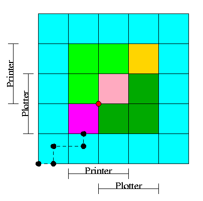
- We have two processes H (horizontal) and V.
- The origin represents them both starting.
- Their combined state is a point on the graph.
- The parts where the printer and plotter are needed by each process
are indicated.
- The dark green is where both processes have the plotter and hence
execution cannot reach this point.
- Light green represents both having the printer; also impossible.
- Pink is both having both printer and plotter; impossible.
- Gold is possible (H has plotter, V has printer), but you can't get
there.
- The upper right corner is the goal; both processes have finished.
- The red dot is ... (cymbals) deadlock. We don't want to go there.
- The cyan is safe. From anywhere in the cyan we have horizontal
and vertical moves to the finish point (the upper right corner)
without hitting any impossible area.
- The magenta interior is very interesting. It is
- Possible: each processor has a different resource
- Not deadlocked: each processor can move within the magenta
- Deadly: deadlock is unavoidable. You will hit a magenta-green
boundary and then will no choice but to turn and go to the red dot.
- The cyan-magenta border is the danger zone.
- The dashed line represents a possible execution pattern.
- With a uniprocessor no diagonals are possible. We either move to
the right meaning H is executing or move up indicating V is executing.
- The trajectory shown represents.
- H excuting a little.
- V excuting a little.
- H executes; requests the printer; gets it; executes some more.
- V executes; requests the plotter.
- The crisis is at hand!
- If the resource manager gives V the plotter, the magenta has been
entered and all is lost. ``Abandon all hope ye who enter here''
--Dante.
- The right thing to do is to deny the request, let H execute moving
horizontally under the magenta and dark green. At the end of the dark
green, no danger remains, both processes will complete successfully.
Victory!
- This procedure is not practical for a general purpose OS since it
requires knowing the programs in advance. That is, the resource
manager, knows in advance what requests each process will make and in
what order.
Homework: 10, 11, 12.
================ Start Lecture #8 ================
3.5.2: Safe States
Avoiding deadlocks given some extra knowledge.
- Not surprisingly, the resource manager knows how many units of each
resource it had to begin with.
- Also it knows how many units of each resource it has given to
each process.
- It would be great to see all the programs in advance and thus know
all future requests, but that is asking for too much.
- Instead, when each process when it starts, it gives its maximum usage.
That is each process at startup states, for each resource, the maximum
number of units it can possibly ask for.
This is called the claim of the process.
- If during the run the process asks for more than its claim,
abort it.
- If it claims more than it needs, the result is that the
resource manager will be more conservative than need be and there
will be more waiting.
Definition: A state is safe
if there is an ordering of the processes such that: if the
processes are run in this order, they will all terminate (assuming
none exceeds its claim).
Give an example of all four possibilities. A state that is
- Safe and deadlocked--not possible
- Safe and not deadlocked
- Not safe and deadlocked
- Not safe and not deadlocked--interesting
A manager can determine if a state is safe.
- Since the manager know all the claims, it can determine the maximum
amount of additional resources each process can request.
- The manager knows how many units of each resource it has left.
The manager then follows the following procedure, which is part of
Banker's Algorithms discovered by Dijkstra, to
determine if the state is safe.
- If there are no processes remaining, the state is
safe.
- Seek a process P whose max additional requests is less than
what remains (for each resource type).
- If no such process can be found, then the state is
not safe.
- The banker (manager) knows that if it refuses all requests
excepts those from P, then it will be able to satisfy all
of P's requests. Why?
Ans: Look at how P was chosen.
- The banker now pretends that P has terminated (since the banker
knows that it can guarantee this will happen). Hence the banker
pretends that all of P's currently held resources are returned. This
makes the banker richer and hence perhaps a process that was not
eligible to be chosen as P previously, can now be chosen.
- Repeat these steps.
Example 1
A safe state with 22 units of one resource
| process | claim | current | max need |
|---|
| X | 3 | 1 | 2 |
| Y | 11 | 5 | 6 |
| Z | 19 | 10 | 9 |
| Total | 16 |
| Available | 6 |
- One resource type R with 22 unit
- Three processes X, Y, and Z with claims 3, 11, and 19 respectively.
- Currently the processes have 1, 5, and 10 units respectively.
- Hence the manager currently has 6 units left.
- Also note that the max additional needs for processes are 2, 6, 9
- So the manager cannot assure (with its current
remaining supply of 6 units) that Z can terminate. But that is
not the question.
- This state is safe
- Use 2 units to satisfy X; now the manager has 7 units.
- Use 6 units to satisfy Y; now the manager has 12 units.
- Use 9 units to satisfy Z; done!
Example 2
A unsafe state with 22 units of one resource
| process | claim | current | max need |
|---|
| X | 3 | 1 | 2 |
| Y | 11 | 5 | 6 |
| Z | 19 | 12 | 7 |
| Total | 18 |
| Available | 4 |
Start with example 1 and assume that Z now requests 2 units and we
grant them.
- Currently the processes have 1, 5, and 12 units respectively.
- The manager has 4 units.
- The max additional needs are 2, 6, and 7.
- This state is unsafe
- Use 2 unit to satisfy X; now the manager has 5 units.
- Y needs 6 and Z needs 7 so we can't guarantee satisfying either
- Note that we were able to find a process that can terminate (X)
but then we were stuck. So it is not enough to find one process.
Must find a sequence of all the processes.
Remark: An unsafe state is not necessarily
a deadlocked state. Indeed, if one gets lucky all processes may
terminate successfully. A safe state means that the manager can
guarantee that no deadlock will occur.
3.5.3: The Banker's Algorithm (Dijkstra) for a Single Resource
The algorithm is simple: Stay in safe states. Initially, we
assume all the processes are present before execution begins and that
all claims are given before execution begins.
We will relax these assumptions very soon.
- Before execution begins, check that the system is safe.
That is, check that no process claims more than the manager has).
If not, then the offending process is trying to claim more than
the system has so cannot be guaranteed to complete even if run by
itself.
You might say that it can become deadlocked all by itself.
- When the manager receives a request, it pretends to grant it and
checks if the resulting state is safe. If it is safe the request is
granted, if not the process is blocked.
- When a resource is returned, the manager (politely thanks the
process and then) checks to see if any of
the pending requests can be granted (i.e., if the result would now be
safe). If so the request is granted and the manager checks to see if
another pending request can be granted, etc..
Homework: 13.
3.5.4: The Banker's Algorithm for Multiple Resources
At a high level the algorithm is identical: Stay in safe states.
- What is a safe state?
- The same definition (if processes are run in a certain order they
will all terminate).
- Checking for safety is the same idea as above. The difference is
that to tell if there enough free resources for a processes to
terminate, the manager must check that for all
resources, the number of free units is at least equal to the max
additional need of the process.
Limitations of the banker's algorithm
- Often users don't know the maximum requests a process will make.
They can estimate conservatively (i.e., use big numbers for the claim)
but then the manager becomes very conservative.
- New processes arriving cause a problem (but not so bad as
Tanenbaum suggests).
- The process's claim must be less than the total number of
units of the resource in the system. If not, the process is not
accepted by the manager.
- Since the state without the new process is safe, so is the
state with the new process! Just use the order you had originally
and put the new process at the end.
- Insuring fairness (starvation freedom) needs a little more
work, but isn't too hard either (once an hour stop taking new
processes until all current processes finish).
- A resource becoming unavailable (e.g., a tape drive breaking), can
result in an unsafe state.
Homework: 21, 27, and 20. There is an interesting
typo in 20 (2nd edition of book): A has claimed 3 units of resource 5,
but there are only 2 units in the entire system. Change A's claim to 2.
3.7: Other Issues
3.7.1: Two-phase locking
This is covered (MUCH better) in a database text. We will skip it.
3.7.2: Non-resource deadlocks
You can get deadlock from semaphores as well as resources. This is
trivial. Semaphores can be considered resources. P(S) is request S
and V(S) is release S. The manager is the module implementing P and
V. When the manager returns from P(S), it has granted the resource S.
3.7.3: Starvation
As usual FCFS is a good cure. Often this is done by priority aging
and picking the highest priority process to get the resource. Also
can periodically stop accepting new processes until all old ones
get their resources.
3.8: Research on Deadlocks
Skipped.
3.9: Summary
Read.
Chapter 4: Memory Management
Also called storage management or
space management.
Memory management must deal with the storage
hierarchy present in modern machines.
- Registers, cache, central memory, disk, tape (backup)
- Move data from level to level of the hierarchy.
- How should we decide when to move data up to a higher level?
- Fetch on demand (e.g. demand paging, which is dominant now).
- Prefetch
- Read-ahead for file I/O.
- Large cache lines and pages.
- Extreme example. Entire job present whenever running.
We will see in the next few lectures that there are three independent
decision:
- Segmentation (or no segmentation)
- Paging (or no paging)
- Fetch on demand (or no fetching on demand)
Memory management implements address translation.
- Convert virtual addresses to physical addresses
- Also called logical to real address translation.
- A virtual address is the address expressed in
the program.
- A physical address is the address understood
by the computer hardware.
- The translation from virtual to physical addresses is performed by
the Memory Management Unit or (MMU).
- Another example of address translation is the conversion of
relative addresses to absolute addresses by the linker.
- The translation might be trivial (e.g., the identity) but not in a modern
general purpose OS.
- The translation might be difficult (i.e., slow).
- Often includes addition/shifts/mask--not too bad.
- Often includes memory references.
- VERY serious.
- Solution is to cache translations in a Translation
Lookaside Buffer (TLB). Sometimes called a
translation buffer (TB).
Homework: 6.
When is address translation performed?
- At compile time
- Compiler generates physical addresses.
- Requires knowledge of where the compilation unit will be loaded.
- No linker.
- Loader is trivial.
- Primitive.
- Rarely used (MSDOS .COM files).
- At link-edit time (the ``linker lab'')
- Compiler
- Generates relocatable addresses for each compilation unit.
- References external addresses.
- Linkage editor
- Converts the relocatable addr to absolute.
- Resolves external references.
- Misnamed ld by unix.
- Also converts virtual to physical addresses by knowing where the
linked program will be loaded. Linker lab ``does'' this,
but it is trivial since we assume the linked program will
be loaded at 0.
- Loader is still trivial.
- Hardware requirements are small.
- A program can be loaded only where specified and
cannot move once loaded.
- Not used much any more.
- At load time
- Similar to at link-edit time, but do not fix
the starting address.
- Program can be loaded anywhere.
- Program can move but cannot be split.
- Need modest hardware: base/limit registers.
- Loader sets the base/limit registers.
- At execution time
- Addresses translated dynamically during execution.
- Hardware needed to perform the virtual to physical address
translation quickly.
- Currently dominates.
- Much more information later.
Extensions
- Dynamic Loading
- When executing a call, check if module is loaded.
- If not loaded, call linking loader to load it and update
tables.
- Slows down calls (indirection) unless you rewrite code dynamically.
- Not used much.
- Dynamic Linking
- The traditional linking described above is today often called
static linking.
- With dynamic linking, frequently used routines are not linked
into the program. Instead, just a stub is linked.
- When the routine is called, the stub checks to see if the
real routine is loaded (it may have been loaded by
another program).
- If not loaded, load it.
- If already loaded, share it. This needs some OS
help so that different jobs sharing the library don't
overwrite each other's private memory.
- Advantages of dynamic linking.
- Saves space: Routine only in memory once even when used
many times.
- Bug fix to dynamically linked library fixes all applications
that use that library, without having to
relink the application.
- Disadvantages of dynamic linking.
- New bugs in dynamically linked library infect all
applications.
- Applications ``change'' even when they haven't changed.
================ Start Lecture #9 ================
Note: I will place ** before each memory management
scheme.
4.1: Basic Memory Management (Without Swapping or Paging)
Entire process remains in memory from start to finish and does not move.
The sum of the memory requirements of all jobs in the system cannot
exceed the size of physical memory.
** 4.1.1: Monoprogramming without swapping or paging (Single User)
The ``good old days'' when everything was easy.
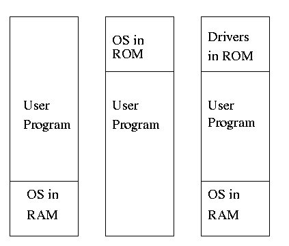
- No address translation done by the OS (i.e., address translation is
not performed dynamically during execution).
- Either reload the OS for each job (or don't have an OS, which is almost
the same), or protect the OS from the job.
- One way to protect (part of) the OS is to have it in ROM.
- Of course, must have the OS (read-write) data in ram.
- Can have a separate OS address space only accessible in
supervisor mode.
- Might just put some drivers in ROM (BIOS).
- The user employs overlays if the memory needed
by a job exceeds the size of physical memory.
- Programmer breaks program into pieces.
- A ``root'' piece is always memory resident.
- The root contains calls to load and unload various pieces.
- Programmer's responsibility to ensure that a piece is already
loaded when it is called.
- No longer used, but we couldn't have gotten to the moon in the
60s without it (I think).
- Overlays have been replaced by dynamic address translation and
other features (e.g., demand paging) that have the system support
logical address sizes greater than physical address sizes.
- Fred Brooks (leader of IBM's OS/360 project and author of ``The
mythical man month'') remarked that the OS/360 linkage editor was
terrific, especially in its support for overlays, but by the time
it came out, overlays were no longer used.
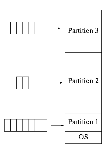
**4.1.2: Multiprogramming with fixed partitions
Two goals of multiprogramming are to improve CPU utilization, by
overlapping CPU and I/O and to permit short jobs to finish quickly.
- This scheme was used by IBM for system 360 OS/MFT
(multiprogramming with a fixed number of tasks).
- Can have a single input queue instead of one for each partition.
- So that if there are no big jobs can use big partition for
little jobs.
- But I don't think IBM did this.
- Can think of the input queue(s) as the ready list(s) with a
scheduling policy of FCFS in each partition.
- The partition boundaries are not movable (must reboot to
move a job).
- MFT can have large internal fragmentation,
i.e., wasted space inside a region
- Each process has a single ``segment'' (we will discuss segments later)
- No sharing between process.
- No dynamic address translation.
- At load time must ``establish addressability''.
- i.e. must set a base register to the location at which the
process was loaded (the bottom of the partition).
- The base register is part of the programmer visible register set.
- This is an example of address translation during load time.
- Also called relocation.
- Storage keys are adequate for protection (IBM method).
- Alternative protection method is base/limit registers.
- An advantage of base/limit is that it is easier to move a job.
- But MFT didn't move jobs so this disadvantage of storage keys is moot.
- Tanenbaum says a job was ``run until it terminates. This must be
wrong as that would mean monoprogramming.
- He probably means that jobs not swapped out and each queue is FCFS
without preemption.
4.1.3: Modeling Multiprogramming
- Consider a job that is unable to compute (i.e., it is waiting for
I/O) a fraction p of the time.
- Then, with monoprogramming, the CPU utilization is 1-p.
- Note that p is often > .5 so CPU utilization is poor.
- But, if the probability that a
job is waiting for I/O is p and n jobs are in memory, then the
probability that all n are waiting for I/O is approximately p^n.
- So, with a multiprogramming level (MPL) of n,
the CPU utilization is approximately 1-p^n.
- If p=.5 and n=4, then 1-p^n = 15/16, which is much better than
1/2, which would occur for monoprogramming (n=1).
- This is a crude model, but it is correct that increasing MPL does
increase CPU utilization up to a point.
- The limitation is memory, which is why we discuss it here
instead of process management. That is, we must have many jobs
loaded at once, which means we must have enough memory for them.
There are other issues as well and we will discuss them.
- Some of the CPU utilization is time spent in the OS executing
context switches so the gains are not a great as the crude model predicts.
Homework: 1, 2 (typo in book; figure 4.21 seems
irrelevant).
4.1.4: Analysis of Multiprogramming System Performance
Skipped
4.1.5: Relocation and Protection
Relocation was discussed as part of linker lab and at the
beginning of this chapter.
When done dynamically, a simple method is to have a
base register whose value is added to every address by the
hardware.
Similarly a limit register is checked by the
hardware to be sure that the address (before the base register is
added) is not bigger than the size of the program.
The base and limit register are set by the OS when the job starts.
4.2: Swapping
Moving entire processes between disk and memory is called
swapping.
Multiprogramming with Variable Partitions
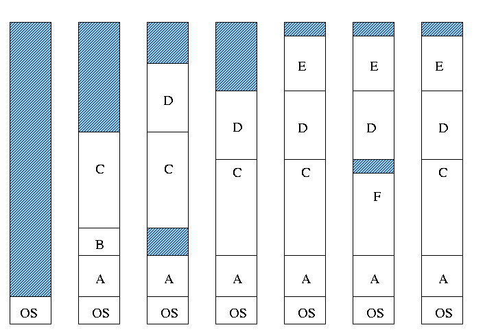 Both the number and size of the partitions change with time.
- IBM OS/MVT (multiprogramming with a varying number of tasks).
- Also early PDP-10 OS.
- Job still has only one segment (as with MFT) but now can be of any
size up to the size of the machine and can change with time.
- A single ready list.
- A job can move (might be swapped back in a different place).
- This is dynamic address translation (during run time).
- Must perform an addition on every memory reference (i.e. on every
address translation) to add the start address of the partition.
- Called a DAT (dynamic address translation) box by IBM.
- Eliminates internal fragmentation.
- Find a region the exact right size (leave a hole for the
remainder).
- Not quite true, can't get a piece with 10A755 bytes. Would
get say 10A760. But internal fragmentation is much
reduced compared to MFT. Indeed, we say that internal
fragmentation has been eliminated.
- Introduces external fragmentation, i.e., holes
outside any region.
- What do you do if no hole is big enough for the request?
- Can compactify
- Transition from bar 3 to bar 4 in diagram below.
- This is expensive.
- Not suitable for real time (MIT ping pong).
- Can swap out one process to bring in another, e.g., bars 5-6
and 6-7 in the diagram.
- There are more processes than holes. Why?
- Because next to a process there might be a process or a hole
but next to a hole there must be a process
- So can have ``runs'' of processes but not of holes
- If after a process equally likely to have a process or a hole,
you get about twice as many processes as holes.
- Base and limit registers are used.
- Storage keys not good since compactifying or moving would require
changing many keys.
- Storage keys might need a fine granularity to permit the
boundaries move by small amounts. Hence many keys would need to be
changed
Homework: 3
MVT Introduces the ``Placement Question''
That is, which hole (partition) should one choose?
- Best fit, worst fit, first fit, circular first fit, quick fit, Buddy
- Best fit doesn't waste big holes, but does leave slivers and
is expensive to run.
- Worst fit avoids slivers, but eliminates all big holes so a
big job will require compaction. Even more expensive than best
fit (best fit stops if it finds a perfect fit).
- Quick fit keeps lists of some common sizes (but has other
problems, see Tanenbaum).
- Buddy system
- Round request to next highest power of two (causes
internal fragmentation).
- Look in list of blocks this size (as with quick fit).
- If list empty, go higher and split into buddies.
- When returning coalesce with buddy.
- Do splitting and coalescing recursively, i.e. keep
coalescing until can't and keep splitting until successful.
- See Tanenbaum for more details (or an algorithms book).
- A current favorite is circular first fit, also know as next fit.
- Use the first hole that is big enough (first fit) but start
looking where you left off last time.
- Doesn't waste time constantly trying to use small holes that
have failed before, but does tend to use many of the big holes,
which can be a problem.
- Buddy comes with its own implementation. How about the others?
4.2.1: Memory Management with Bitmaps
Divide memory into blocks and associate a bit with each block, used
to indicate if the corresponding block is free or allocated. To find
a chunk of size N blocks need to find N consecutive bits
indicating a free block.
The only design question is how much memory does one bit represent.
- Big: Serious internal fragmentation.
- Small: Many bits to store and process.
4.2.2: Memory Management with Linked Lists
- Each item on list gives the length and starting location of the
corresponding region of memory and says whether it is a Hole or Process.
- The items on the list are not taken from the memory to be
used by processes.
- Keep in order of starting address.
- Merge adjacent holes
- Double linked
Memory Management using Boundary Tags
- Use the same memory for list items as for processes
- Don't need an entry in linked list for blocks in use, just
the avail blocks are linked.
- For the blocks currently in use, just need a hole/process bit at
each end and the length. Keep this in the block itself.
- See Knuth, The Art of Computer Programming vol 1.
Homework: 5.
MVT also introduces the ``Replacement Question''
That is, which victim should we swap out?
Note that this is an example of the suspend arc mentioned in process
scheduling.
We will study this question more when we discuss
demand paging in which case
we swap out part of a process.
Considerations in choosing a victim
- Cannot replace a job that is pinned,
i.e. whose memory is tied down. For example, if Direct Memory
Access (DMA) I/O is scheduled for this process, the job is pinned
until the DMA is complete.
- Victim selection is a medium term scheduling decision
- A job that has been in a wait state for a long time is a good
candidate.
- Often choose as a victim a job that has been in memory for a long
time.
- Another question is how long should it stay swapped out.
- For demand paging, where swaping out a page is not as drastic as
swapping out a job, choosing the victim is an important memory
management decision and we shall study several policies,
================ Start Lecture #10 ================
NOTEs:
- So far the schemes presented so far have had two properties:
- Each job is stored contiguously in memory. That is, the job is
contiguous in physical addresses.
- Each job cannot use more memory than exists in the system. That
is, the virtual addresses space cannot exceed the physical address
space.
- Tanenbaum now attacks the second item. I wish to do both and start
with the first.
- Tanenbaum (and most of the world) uses the term ``paging'' to mean
what I call demand paging. This is unfortunate as it mixes together
two concepts.
- Paging (dicing the address space) to solve the placement
problem and essentially eliminate external fragmentation.
- Demand fetching, to permit the total memory requirements of
all loaded jobs to exceed the size of physical memory.
- Tanenbaum (and most of the world) uses the term virtual memory as
a synonym for demand paging. Again I consider this unfortunate.
- Demand paging is a fine term and is quite descriptive.
- Virtual memory ``should'' be used in contrast with physical
memory to describe any virtual to physical address translation.
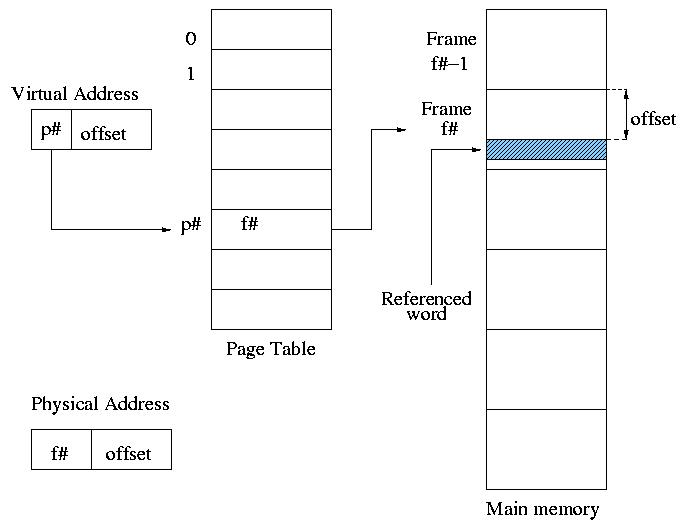
** (non-demand) Paging
Simplest scheme to remove the requirement of contiguous physical
memory.
- Chop the program into fixed size pieces called
pages (invisible to the programmer).
- Chop the real memory into fixed size pieces called page
frames or simply frames.
- Size of a page (the page size) = size of a frame (the frame size).
- Sprinkle the pages into the frames.
- Keep a table (called the page table) having an
entry for each page. The page table entry or PTE for
page p contains the number of the frame f that contains page p.
Example: Assume a decimal machine with
page size = frame size = 1000.
Assume PTE 3 contains 459.
Then virtual address 3372 corresponds to physical address 459372.
Properties of (non-demand) paging.
- Entire job must be memory resident to run.
- No holes, i.e. no external fragmentation.
- If there are 50 frames available and the page size is 4KB than a
job requiring <= 200KB will fit, even if the available frames are
scattered over memory.
- Hence (non-demand) paging is useful.
- Introduces internal fragmentation approximately equal to 1/2 the
page size for every process (really every segment).
- Can have a job unable to run due to insufficient memory and
have some (but not enough) memory available. This is not
called external fragmentation since it is not due to memory being fragmented.
- Eliminates the placement question. All pages are equally
good since don't have external fragmentation.
- The replacement question remains.
- Since page boundaries occur at ``random'' points and can change from
run to run (the page size can change with no effect on the
program--other than performance), pages are not appropriate units of
memory to use for protection and sharing. This is discussed further
when we introduce segmentation.
Homework: 16.
Address translation
- Each memory reference turns into 2 memory references
- Reference the page table
- Reference central memory
- This would be a disaster!
- Hence the MMU caches page#-->frame# translations. This cache is kept
near the processor and can be accessed rapidly.
- This cache is called a translation lookaside buffer (TLB) or
translation buffer (TB).
- For the above example, after referencing virtual address 3372,
there would be an entry in the TLB containing the mapping
3-->459.
- Hence a subsequent access to virtual address 3881 would be
translated to physical address 459881 without a memory reference.
Choice of page size is discuss below.
Homework: 8.
4.3: Virtual Memory (meaning fetch on demand)
Idea is that a program can execute even if only the active portion of its
address space is memory resident. That is, swap in and swap out
portions of a program. In a crude sense this can be called
``automatic overlays''.
Advantages
- Can run a program larger than the total physical memory.
- Can increase the multiprogramming level since the total size of
the active, i.e. loaded, programs (running + ready + blocked) can
exceed the size of the physical memory.
- Since some portions of a program are rarely if ever used, it is
an inefficient use of memory to have them loaded all the time. Fetch on
demand will not load them if not used and will unload them during
replacement if they are not used for a long time (hopefully).
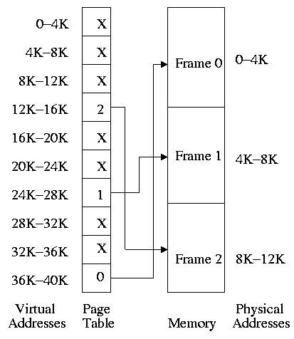
4.3.1: Paging (meaning demand paging)
Fetch pages from disk to memory when they are referenced, with a hope
of getting the most actively used pages in memory.
- Very common: dominates modern operating systems.
- Started by the Atlas system at Manchester University in the 60s
(Fortheringham).
- Each PTE continues to have the frame number if the page is
loaded.
- But what if the page is not loaded (exists only on disk)?
- The PTE has a flag indicating if it is loaded (can think of
the X in the diagram on the right as indicating that this flag is
not set).
- If not loaded, the location on disk could be kept in the PTE
(not shown in the diagram). But normally it is not
(discussed below).
- When a reference is made to a non-loaded page (sometimes
called a non-existent page, but that is a bad name), the system
has a lot of work to do. We give more details
below.
- Choose a free frame, if one exists.
- If not
- Choose a victim frame.
- More later on how to choose a victim.
- Called the replacement question
- Write victim back to disk if dirty,
- Update the victim PTE to show that it is not loaded
and, perhaps, where on disk it has been put.
- Copy the referenced page from disk to the free frame.
- Update the PTE of the referenced page to show that it is
loaded and give the frame number.
- Do the standard paging address translation (p#,off)-->(f#,off).
- Really not done quite this way
- There is ``always'' a free frame because ...
- There is a deamon active that checks the number of free frames
and if this is too low, chooses victims and ``pages them out''
(writing them back to disk if dirty).
- Choice of page size is discussed below.
Homework: 12.
4.3.2: Page tables
A discussion of page tables is also appropriate for (non-demand)
paging, but the issues are more acute with demand paging since the
tables can be much larger. Why?
- The total size of the active processes is no longer limited to
the size of physical memory. Since the total size of the processes is
greater, the total size of the page tables is greater and hence
concerns over the size of the page table are more acute.
- With demand paging an important question is the choice of a victim
page to page out. Data in the page table
can be useful in this choice.
We must be able access to the page table very quickly since it is
needed for every memory access.
Unfortunate laws of hardware.
- Big and fast are essentially incompatible.
- Big and fast and low cost is hopeless.
So we can't just say, put the page table in fast processor registers,
and let it be huge, and sell the system for $1500.
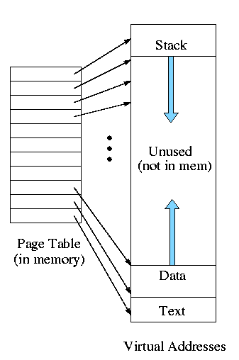
For now, put the (one-level) page table in main memory.
- Seems too slow since all memory references require two reference.
- TLB very helpful to reduce the average delay as mentioned above
(discussed later in more detail).
- The page table might be too big.
- Currently we are considering contiguous virtual
addresses ranges (i.e. the virtual addresses have no holes).
- Typically put the stack at one end of virtual address and the
global (or static) data at the other end and let them grow towards
each other.
- The memory in between is unused.
- This unused memory can be huge (in address range) and hence
the page table will mostly contain unneeded PTEs.
- Works fine if the maximum virtual address size is small, which
was once true (e.g., the PDP-11 of the 1970s) but is no longer the
case.
Contents of a PTE
Each page has a corresponding page table entry (PTE). The
information in a PTE is for use by the hardware. Information set by
and used by the OS is normally kept in other OS tables. The page
table format is determined by the hardware so access routines are not
portable. The following fields are often present.
- The valid bit. This tells if
the page is currently loaded (i.e., is in a frame). If set, the frame
pointer is valid. It is also called the presence or
presence/absence bit. If a page is accessed with the valid
bit zero, a page fault is generated by the hardware.
- The frame number. This is the main reason for the table. It is
needed for virtual to physical address translation.
- The Modified bit. Indicates that some part of the page
has been written since it was loaded. This is needed when the page is
evicted so the OS can know that the page must be written back to disk.
- The referenced bit. Indicates that some word in the page
has been referenced. Used to select a victim: unreferenced pages make
good victims by the locality property (discussed below).
- Protection bits. For example one can mark text pages as
execute only. This requires that boundaries between regions with
different protection are on page boundaries. Normally many
consecutive (in logical address) pages have the same protection so
many page protection bits are redundant.
Protection is more
naturally done with segmentation.
Multilevel page tables (Not on 202 final exam)
Recall the previous diagram. Most of the virtual memory is the
unused space between the data and stack regions. However, with demand
paging this space does not waste real memory. But the single
large page table does waste real memory.
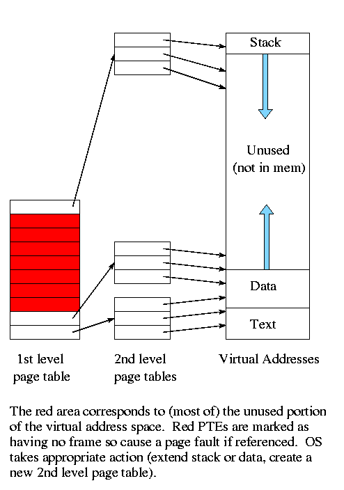
The idea of multi-level page tables (a similar idea is used in Unix
i-node-based file systems) is to add a level of indirection and have a
page table containing pointers to page tables.
- Imagine one big page table.
- Call it the second level page table and
cut it into pieces each the size of a page.
Note that you can get many PTEs in one page so you will have far
fewer of these pages than PTEs
- Now construct a first level page table containing PTEs that point to
these pages.
- This first level PT is small enough to store in memory.
- But since we still have the 2nd level PT, we have made the world
bigger not smaller!
- Don't store in memory those 2nd level page tables all of whose PTEs
refer to unused memory. That is use demand paging on the (second
level) page table
Do an example on the board
The VAX used a 2-level page table structure, but with some wrinkles
(see Tanenbaum for details).
Naturally, there is no need to stop at 2 levels. In fact the SPARC
has 3 levels and the Motorola 68030 has 4 (and the number of bits of
Virtual Address used for P#1, P#2, P#3, and P#4 can be varied).
4.3.3: TLBs--Translation Lookaside Buffers (and General
Associative Memory)
Note:
Tanenbaum suggests that ``associative memory'' and ``translation
lookaside buffer'' are synonyms. This is wrong. Associative memory
is a general structure and translation lookaside buffer is a special
case.
An
associative memory is a content addressable
memory. That is you access the memory by giving the value
of some field and the hardware searches all the records and returns
the record whose field contains the requested value.
For example
Name  | Animal | Mood     | Color
======+========+==========+======
Moris | Cat    | Finicky  | Grey
Fido  | Dog    | Friendly | Black
Izzy  | Iguana | Quiet    | Brown
Bud   | Frog   | Smashed  | Green
If the index field is Animal and Iguana is given, the associative
memory returns
Izzy | Iguana | Quiet | Brown
A Translation Lookaside Buffer
or TLB
is an associate memory
where the index field is the page number. The other fields include
the frame number, dirty bit, valid bit, and others.
-
A TLB is small and expensive but at least it is
fast. When the page number is in the TLB, the frame number
is returned very quickly.
-
On a miss, the page number is looked up in the page table. The record
found is placed in the TLB and a victim is discarded. There is no
placement question since all entries are accessed at the same time.
But there is a replacement question.
Homework: 17.
4.3.4: Inverted page tables
Keep a table indexed by frame number with the entry f containing the
number of the page currently loaded in frame f.
- Since modern machine have a smaller physical address space than
virtual address space, the table is smaller
- But on a TLB miss, must search the inverted page table.
- Would be hopelessly slow except that some tricks are employed.
- The book mentions some but not all of the tricks, we are skipping
this topic.
================ Start Lecture #11 ================
4.4: Page Replacement Algorithms (PRAs)
These are solutions to the replacement question.
Good solutions take advantage of locality.
- Temporal locality: If a word is referenced now,
it is likely to be referenced in the near future.
- This argues for caching referenced words,
i.e. keeping the referenced word near the processor for a while.
- Spatial locality: If a word is referenced now,
nearby words are likely to be referenced in the near future.
- This argues for prefetching words around the currently
referenced word.
- These are lumped together into locality: If any
word in a page is referenced, each word in the page is ``likely'' to
be referenced.
- So it is good to bring in the entire page on a miss and to
keep the page in memory for a while.
- When programs begin there is no history so nothing to base
locality on. At this point the paging system is said to be undergoing
a ``cold start''.
- Programs exhibit ``phase changes'', when the set of pages referenced
changes abruptly (similar to a cold start). At the point of a phase
change, many page faults occur because locality is poor.
Pages belonging to processes that have terminated are of course
perfect choices for victims.
Pages belonging to processes that have been blocked for a long time
are good choices as well.
Random PRA
A lower bound on performance. Any decent scheme should do better.
4.4.1: The optimal page replacement algorithm (opt PRA) (aka
Belady's min PRA)
Replace the page whose next
reference will be furthest in the future.
- Also called Belady's min algorithm.
- Provably optimal. That is, generates the fewest number of page
faults.
- Unimplementable: Requires predicting the future.
- Good upper bound on performance.
4.4.2: The not recently used (NRU) PRA
Divide the frames into four classes and make a random selection from
the lowest nonempty class.
- Not referenced, not modified
- Not referenced, modified
- Referenced, not modified
- Referenced, modified
Assumes that in each PTE there are two extra flags R (sometimes called
U, for used) and M (often called D, for dirty).
Also assumes that a page in a lower priority class is cheaper to evict.
- If not referenced, probably will not referenced again soon and
hence is a good candidate for eviction.
- If not modified, do not have to write it out so the cost of the
eviction is lower.
- When a page is brought in, OS resets R and M (i.e. R=M=0)
- On a read, hardware sets R.
- On a write, hardware sets R and M.
We again have the prisoner problem, we do a good job of making little
ones out of big ones, but not the reverse. Need more resets.
Every k clock ticks, reset all R bits
- Why not reset M?
Answer: Must have M accurate to know if victim needs to be written back
- Could have two M bits one accurate and one reset, but I don't know
of any system (or proposal) that does so.
What if the hardware doesn't set these bits?
- OS can use tricks
- When the bits are reset, make the PTE indicate the page is not
resident (i.e. lie). On the page fault, set the appropriate bit(s).
4.4.3: FIFO PRA
Simple but poor since usage of the page is ignored.
Belady's Anomaly: Can have more frames yet generate
more faults.
Example given later.
4.4.4: Second chance PRA
Similar to the FIFO PRA but when time choosing a victim, if the page
at the head of the queue has been referenced (R bit set), don't evict
it.
Instead reset R and move the page to the rear of the queue (so it
looks new).
The page is being a second chance.
What if all frames have been referenced?
Becomes the same as fifo (but takes longer).
Might want to turn off the R bit more often (say every k clock ticks).
4.4.5: Clock PRA
Same algorithm as 2nd chance, but a better (and I would say obvious)
implementation: Use a circular list.
Do an example.
LIFO PRA
This is terrible! Why?
Ans: All but the last frame are frozen once loaded so you can replace
only one frame. This is especially bad after a phase shift in the
program when it is using all new pages.
4.4.6:Least Recently Used (LRU) PRA
When a page fault occurs, choose as victim that page that has been
unused for the longest time, i.e. that has been least recently used.
LRU is definitely
- Implementable: The past is knowable.
- Good: Simulation studies have shown this.
- Difficult. Essentially need to either:
- Keep a time stamp in each PTE, updated on each reference
and scan all the PTEs when choosing a victim to find the PTE
with the oldest timestamp.
- Keep the PTEs in a linked list in usage order, which means
on each reference moving the PTE to the end of the list
Homework: 29, 23
A hardware cutsie in Tanenbaum
- For n pages, keep an nxn bit matrix.
- On a reference to page i, set row i to all 1s and col i to all 0s
-
At any time the 1 bits in the rows are ordered by inclusion. I.e. one
row's 1s are a subset of another row's 1s, which is a subset of a
third. (Tanenbaum forgets to mention this.)
-
So the row with the fewest 1s is a subset of all the others and is
hence least recently used
- Cute, but still impractical.
4.4.7: Simulating (Approximating) LRU in Software
The Not Frequently Used (NFU) PRA
- Include a counter in each PTE (and have R in each PTE).
- Set counter to zero when page is brought into memory.
- For each PTE, every k clock ticks.
- Add R to counter.
- Clear R.
- Choose as victim the PTE with lowest count.
| R | counter |
|---|
| 1 | 10000000 |
|
| 0 | 01000000 |
|
| 1 | 10100000 |
|
| 1 | 11010000 |
|
| 0 | 01101000 |
|
| 0 | 00110100 |
|
| 1 | 10011010 |
|
| 1 | 11001101 |
|
| 0 | 01100110 |
|
The Aging PRA
NFU doesn't distinguish between old references and recent ones. The
following modification does distinguish.
- Include a counter in each PTE (and have R in each PTE).
- Set counter to zero when page is brought into memory.
- For each PTE, every k clock ticks.
- Shift counter right one bit.
- Insert R as new high order bit (HOB).
- Clear R.
- Choose as victim the PTE with lowest count.
Homework: 25, 34
4.4.8: The Working Set Page Replacement Problem (Peter Denning)
The working set policy (Peter Denning)
The goal is to specify which pages a given process needs to have
memory resident in order for the give process to run without too many
page faults.
- But this is impossible since it requires predicting the future.
- So we make the assumption that the immediate future is well
approximated by the immediate past.
- Measure time in units of memory references, so t=1045 means the time
when the 1045th memory reference is issued.
- In fact we measure time separately
for each process, so t=1045 really means the time when this process
made its 1045th memory reference.
- W(t,&omega) is the set of pages referenced (by the given process) from
time t-ω to time t.
- That is, W(t,ω) is the set pages referenced during
the window of size ω ending at time t.
- That is, W(t,ω) is the set of pages referenced by the last
ω memory references ending at reference t.
- W(t,ω) is called the working set at time t
(with window ω).
- Does this Netscape support the ω notation to give the Greek letter?
- w(t,ω) is the size of the set W(t,ω), i.e. is the
number of pages referenced in the window.
The idea of the working set policy is to ensure that each process
keeps its working set in memory.
- Allocate w(t,ω) frames to each process.
This number differs for each process and changes with time.
- On a fault, one replaces a page not in the working set. But it is
not easy to find such a page quickly.
- Indeed determining W(t,ω) is difficult.
- We will see that the working set algorithm is essentially a
``global policy'' (defined below). I would actually prefer
covering the working set policy after defining local and global
policies but decided to follow Tannenbaum.
- If a process is suspended, it is often swapped out; the working
set then can be used to say which pages should be brought back
when the process is resumed.
Interesting questions include:
- What value should be used for ω?
Experiments have been done and ω is surprisingly robust (i.e.,
for a given system a fixed value works reasonably for a wide variety
of job mixes)
- How should we calculate W(t,ω)?
Hard so do exactly so ...
... Various approximations to the working set, have been devised.
We will study three: using virtual time instead of memory references
(immediately below),
WSClock (section 4.4.9), and Page Fault Frequency (section 4.6).
Using virtual time
Approximate the working set as those pages referenced during the
last m milliseconds.
Then clear the reference bit every m milliseconds and set it on every
reference.
Note that the time is measured only while this process is running.
That is why it is called virtual time.
So now to choose a victim, we need to find a page with the R bit
clear.
Similar to NRU.
4.4.9: The WSClock Page Replacement Algorithm
- Use the aging algorithm above to maintain a counter for
each PTE and declare a page whose counter is above a certain threshold
to be part of the working set.
- Apply the clock algorithm globally (i.e. to all pages) but
refuse to page out any page in a working set.
The resulting algorithm is called wsclock.
- What if we find there are no pages we can page out?
Simple answer: Pick some page (almost at random).
Another answer: Reduce the multiprogramming level
(explained in 4.6 below).
4.4.10: Summary of Page Replacement Algorithms
| Algorithm | Comment
|
|---|
| Random | Poor, used for comparison
|
| Optimal | Unimplementable, use for comparison
|
| LIFO | Horrible, useless
|
| NRU | Crude
|
| FIFO | Not good ignores frequency of use
|
| Second Chance | Improvement over FIFO
|
| Clock | Better (natural) implementation of Second Chance
|
| LRU | Great but impractical
|
| NFU | Crude LRU approximation
|
| Aging | Better LRU approximation
|
| Working Set | Good, but expensive
|
| WSClock | Good approximation to working set
|
4.5: Modeling Paging Algorithms
4.5.1: Belady's anomaly
Consider a system that has no pages loaded and that uses the FIFO
PRU.
Consider the following ``reference string'' (sequences of pages referenced).
0 1 2 3 0 1 4 0 1 2 3 4
If we have 3 frames this generates 9 page faults (do it).
If we have 4 frames this generates 10 page faults (do it).
Theory has been developed and certain PRA (so called ``stack
algorithms'') cannot suffer this anomaly for any reference string.
FIFO is clearly not a stack algorithm. LRU is. Tannenbaum has a few
details, but we are skipping it.
Repeat the above calculations for LRU.
4.6: Design issues for (demand) Paging Systems
4.6.1: Local vs Global Allocation Policies
A local PRA is one is which a victim page is chosen
among the pages of the same process that requires a new page. That is
the number of pages for each process is fixed. So LRU means the page
least recently used by this process.
- Of course we can't have a purely local policy, why?
Answer: A new process has no pages and even if we didn't apply this for
the first page loaded, the process would remain with only one page.
- Perhaps wait until a process has been running a while or give
the process an initial allocation based on the size of the executable.
- A global policy is one in which the choice of
victim is made among all pages of all processes.
If we apply global LRU indiscriminately with some sort of RR processor
scheduling policy, and memory is somewhat over-committed, then by the
time we get around to a process, all the others have run and have
probably paged out this process.
If this happens each process will need to page fault at a high
rate; this is called thrashing.
It is therefore important to get a good
idea of how many pages a process needs, so that we can balance the
local and global desires. The working set W(t,ω) is good for
this.
An approximation to the working set policy that is useful for
determining how many frames a process needs (but not which pages)
is the Page Fault Frequency (PFF) algorithm.
- For each process keep track of the page fault frequency, which
is the number of faults divided by the number of references.
- Actually, must use a window or a weighted calculation since
you are really interested in the recent page fault frequency.
- If the PFF is too high, allocate more frames to this process.
Either
- Raise its number of frames and use a local policy; or
- Bar its frames from eviction (for a while) and use a
global policy.
- What if there are not enough frames?
Answer: Reduce the MPL (see next section).
As mentioned above a question arises what to do if the sum of the
working set sizes exceeds the amount of physical memory available.
This question is similar to the final point about PFF and brings us to
consider controlling the load (or memory pressure).
4.6.2: Load Control
To reduce the overall memory pressure, we must reduce the
multiprogramming level (or install more memory while the system is
running, which is hardly practical). That is, we have a
connection between memory management and process management. This is
the suspend/resume arcs we saw way back when.
================ Start Lecture #12 ================
4.6.3: Page size
- Page size ``must'' be a multiple of the disk block size. Why?
Answer: When copying out a page if you have a partial disk block, you
must do a read/modify/write (i.e., 2 I/Os).
- Important property of I/O that we will learn later this term is
that eight I/Os each 1KB takes considerably longer than one 8KB I/O
- Characteristics of a large page size.
- Good for user I/O.
- If I/O done using physical addresses, then I/O crossing a
page boundary is not contiguous and hence requires multiple
I/Os
- If I/O uses virtual addresses, then page size doesn't effect
this aspect of I/O. That is the addresses are contiguous
in virtual address and hence one I/O is done.
- Good for demand paging I/O.
- Better to swap in/out one big page than several small
pages.
- But if page is too big you will be swapping in data that is
really not local and hence might well not be used.
- Large internal fragmentation (1/2 page size).
- Small page table.
- A very large page size leads to very few pages. Process will
have many faults if using demand
paging and the process frequently references more regions than
frames.
- A small page size has the opposite characteristics.
4.6.4: Separate Instruction and Data (I and D) Spaces
Skipped.
4.6.5: Shared pages
Permit several processes to each have a page loaded in the same
frame.
Of course this can only be done if the processes are using the same
program and/or data.
- Really should share segments.
- Must keep reference counts or something so that when a process
terminates, pages (even dirty pages) it shares with another process
are not automatically discarded.
- Similarly, a reference count would make a widely shared page (correctly)
look like a poor choice for a victim.
- A good place to store the reference count would be in a structure
pointed to by both PTEs. If stored in the PTEs, must keep them
consistent between processes.
4.6.6: Cleaning Policy (Paging Daemons)
Done earlier
4.6.7: Virtual Memory Interface
Skipped.
4.7: Implementation Issues
4.7.1: Operating System Involvement with Paging
4.7.2: Page Fault Handling
What happens when a process, say process A, gets a page fault?
- The hardware detects the fault and traps to the kernel (switches
to supervisor mode and saves state).
- Some assembly language code save more state, establishes the
C-language (or another programming language) environment, and
``calls'' the OS.
- The OS determines that a page fault occurred and which page was
referenced.
- If the virtual address is invalid, process A is killed.
If the virtual address is valid, the OS must find a free frame.
If there is no free frames, the OS selects a victim frame.
Call the process owning the victim frame, process B.
(If the page replacement algorithm is local, the victim is process A.)
- The PTE of the victim page is updated to show that the page is no
longer resident.
- If the victim page is dirty, the OS schedules an I/O write to
copy the frame to disk and blocks A waiting for this I/O to occur.
- Since process A is blocked, the scheduler is invoked to perform a
context switch.
- Tanenbaum ``forgot'' some here.
- The process selected by the scheduler (say process C) runs.
- Perhaps C is preempted for D or perhaps C blocks and D runs
and then perhaps D is blocked and E runs, etc.
- When the I/O to write the victim frame completes, a Disk
interrupt occurs. Assume processes C is running at the time.
- Hardware trap / assembly code / OS determines I/O done.
- The scheduler picks a process to run, maybe A, maybe B, maybe
C, maybe another processes.
- At some point the scheduler does pick process A to run.
Recall that at this point A is still executing OS code.
- Now the O/S has a clean frame (this may be much later in wall clock
time if a victim frame had to be written).
The O/S schedules an I/O to read the desired page into this clean
frame.
Process A is blocked (perhaps for the second time) and hence the
process scheduler is invoked to perform a context switch.
- A Disk interrupt occurs when the I/O completes (trap / asm / OS
determines I/O done). The PTE in process A is updated to indicate
that the page is in memory.
- The O/S may need to fix up process A (e.g. reset the program
counter to re-execute the instruction that caused the page fault).
- Process A is placed on the ready list and eventually is chosen by
the scheduler to run.
Recall that process A is executing O/S code.
- The OS returns to the first assembly language routine.
- The assembly language routine restores registers, etc. and
``returns'' to user mode.
The user's program running as process A is unaware
that all this happened (except for the time delay).
4.7.3: Instruction Backup
A cute horror story. The 68000 was so bad in this regard that
early demand paging systems for the 68000, used two processors one
running one instruction behind. If the first got a page fault, there
wasn't always enough information to figure out what to do so the
system switched to the second processor after it did the page fault.
Don't worry about instruction backup. Very machine dependent and
modern implementations tend to get it right. The next generation
machine, 68010, provided extra information on the stack so the
horrible 2-processor kludge was no longer necessary.
4.7.4: Locking (Pinning) Pages in Memory
We discussed pinning jobs already. The
same (mostly I/O) considerations apply to pages.
4.7.5: Backing Store
The issue is where on disk do we put pages.
- For program text, which is presumably read only, a good choice is
the file itself.
- What if we decide to keep the data and stack each contiguous on
the backing store.
Data and stack grow so we must be prepared to grow the space on
disk, which leads to the same issues and problems as we saw with
MVT.
- If those issues/problems are painful, we can scatter the pages on
the disk.
- That is we employ paging!
- This is NOT demand paging.
- Need a table to say where the backing space for each page is
located.
- This corresponds to the page table used to tell where in
real memory a page is located.
- The format of the ``memory page table'' is determined by
the hardware since the hardware modifies/accesses it.
- The format of the ``disk page table'' is decided by the OS
designers and is machine independent.
- If the format of the memory page table was flexible, then
we might well keep the disk information in it as well.
- What if we felt disk space was too expensive and wanted to put some of
these disk pages on say tape?
Ans: We have demand paging of the disk blocks!
4.7.6: Separation of Policy and Mechanism
Skipped.
4.8: Segmentation
Up to now, the virtual address space has been contiguous.
- Among other issues this makes memory management difficult when
there are more that two dynamically growing regions.
- With two regions you start them on opposite sides of the virtual
space as we did before.
- Better is to have many virtual address spaces each starting at
zero.
- This split up is user visible.
- Without segmentation (equivalently said with just one segment) all
procedures are packed together so if one changes in size all the virtual
addresses following are changed and the program must be re-linked.
- Eases flexible protection and sharing (share a segment). For
example, can have a shared library.
Homework: 37.
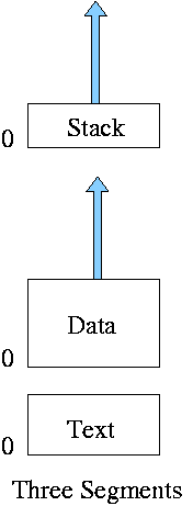
** Two Segments
Late PDP-10s and TOPS-10
- One shared text segment, that can also contain shared
(normally read only) data.
- One (private) writable data segment.
- Permission bits on each segment.
- Which kind of segment is better to evict?
- Swap out shared segment hurts many tasks.
- The shared segment is read only (probably) so no writeback
is needed.
- ``One segment'' is OS/MVT done above.
** Three Segments
Traditional (early) Unix shown at right.
- Shared text marked execute only.
- Data segment (global and static variables).
- Stack segment (automatic variables).
- In reality, since the text doesn't grow, this was sometimes
treated as 2 segments by combining text and data into one segment
** Four Segments
Just kidding.
** General (not necessarily demand) Segmentation
- Permits fine grained sharing and protection. For a simple example
can share the text segment in early unix.
- Visible division of program.
- Variable size segments.
- Virtual Address = (seg#, offset).
- Does not mandate how stored in memory.
- One possibility is that the entire program must be in memory
in order to run it.
Use whole process swapping.
Very early versions of Unix did this.
- Can also implement demand segmentation.
- Can combine with demand paging (done below).
- Requires a segment table with a base and limit value for each
segment. Similar to a page table. Why is there no limit value in a
page table?
Ans: All pages are the same size so the limit is obvious.
- Entries are called STEs, Segment Table Entries.
- (seg#, offset) --> if (offset<limit) base+offset else error.
- Segmentation exhibits external fragmentation, just as whole program
swapping.
Since segments are smaller than programs (several segments make up one
program), the external fragmentation is not as bad.
** Demand Segmentation
Same idea as demand paging applied to segments.
- If a segment is loaded, base and limit are stored in the STE and
the valid bit is set in the PTE.
- The PTE is accessed for each memory reference (not really, TLB).
- If the segment is not loaded, the valid bit is unset.
The base and limit as well as the disk
address of the segment is stored in the an OS table.
- A reference to a non-loaded segment generate a segment fault
(analogous to page fault).
- To load a segment, we must solve both the placement question and the
replacement question (for demand paging, there is no placement question).
- I believe demand segmentation was once implemented by Burroughs,
but am not sure.
It is not used in modern systems.
The following table mostly from Tanenbaum compares demand
paging with demand segmentation.
| Consideration |
Demand
Paging | Demand
Segmentation |
|---|
| Programmer aware |
No | Yes |
| How many addr spaces |
1 | Many |
| VA size > PA size |
Yes | Yes |
Protect individual
procedures separately |
No | Yes |
Accommodate elements
with changing sizes |
No | Yes |
| Ease user sharing |
No | Yes |
| Why invented |
let the VA size
exceed the PA size |
Sharing, Protection,
independent addr spaces |
|
| Internal fragmentation |
Yes | No, in principle |
| External fragmentation |
No | Yes |
| Placement question |
No | Yes |
| Replacement question |
Yes | Yes |
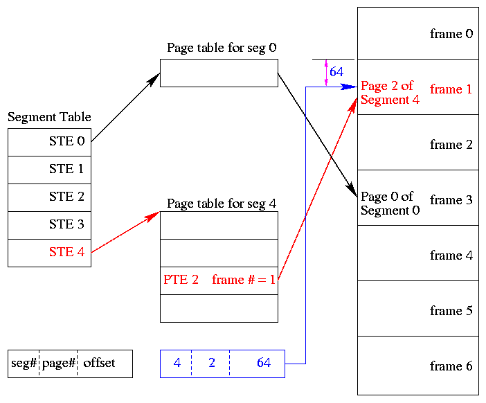
** 4.8.2 and 4.8.3: Segmentation With Paging
(Tanenbaum gives two sections to explain the differences between
Multics and the Intel Pentium. These notes cover what is common to
all segmentation).
Combines both segmentation and paging to get advantages of both at
a cost in complexity. This is very common now.
- A virtual address becomes a triple: (seg#, page#, offset).
- Each segment table entry (STE) points to the page table for that
segment.
Compare this with a
multilevel page table.
- The size of each segment is a multiple of the page size (since the
segment consists of pages). Perhaps not. Can keep the exact size in
the STE (limit value) and shoot the process if it referenced beyond
the limit. In this case the last page of each segment is partially valid.
- The page# field in the address gives the entry in the chosen page
table and the offset gives the offset in the page.
- From the limit field, one can easily compute the size of the
segment in pages (which equals the size of the corresponding page
table in PTEs). Implementations may require the size of a segment to
be a multiple of the page size in which case the STE would store the
number of pages in the segment.
- A straightforward implementation of segmentation with paging
would requires 3 memory references (STE, PTE, referenced word) so a
TLB is crucial.
- Some books carelessly say that segments are of fixed size.
This is wrong.
They are of variable size with a fixed maximum and possibly with the
requirement that the size of a segment is a multiple of the page size.
- The first example of segmentation with paging was Multics.
- Keep protection and sharing information on segments.
This works well for a number of reasons.
- A segment is variable size.
- Segments and their boundaries are user (i.e., linker) visible.
- Segments are shared by sharing their page tables. This
eliminates the problem mentioned above with
shared pages.
- Do replacement on pages so there is no placement question and
no external fragmentation.
- Do fetch-on-demand with pages (i.e., do demand paging).
- In general, segmentation with demand paging works well and is
widely used. The only problems are the complexity and the resulting 3
memory references for each user memory reference. The complexity is
real, but can be managed. The three memory references would be fatal
were it not for TLBs, which considerably ameliorate the problem. TLBs
have high hit rates and for a TLB hit there is essentially no penalty.
Homework: 38.
4.9: Research on Memory Management
Skipped
4.10: Summary
Read
Some Last Words on Memory Management
- Segmentation / Paging / Demand Loading (fetch-on-demand)
- Each is a yes or no alternative.
- Gives 8 possibilities.
- Placement and Replacement.
- Internal and External Fragmentation.
- Page Size and locality of reference.
- Multiprogramming level and medium term scheduling.
================ Start Lecture #13 ================
Chapter 5: Input/Output
5.1: Principles of I/O Hardware
5.1.1: I/O Devices
- Not much to say. Devices are varied.
- Block versus character devices:
- Devices, such as disks and CDROMs, with addressable chunks
(sectors in this case) are called block
devices,
These devices support seeking.
- Devices, such as Ethernet and modem connections, that are a
stream of characters are called character
devices.
These devices do not support seeking.
- Some cases, like tapes, are not so clear.
5.1.2: Device Controllers
These are the ``devices'' as far as the OS is concerned. That
is, the OS code is written with the controller spec in hand not with
the device spec.
- Also called adaptors.
- The controller abstracts away some of the low level features of
the device.
- For disks, the controller does error checking and buffering.
- (Unofficial) In the old days it handled interleaving of sectors.
(Sectors are interleaved if the
controller or CPU cannot handle the data rate and would otherwise have
to wait a full revolution. This is not a concern with modern systems
since the electronics have increased in speed faster than the
devices.)
- For analog monitors (CRTs) the controller does
a great deal. Analog video is far from a bunch of ones and
zeros.
- Controllers are also called adaptors.
5.1.3: Memory-Mapped I/O
Think of a disk controller and a read request. The goal is to copy
data from the disk to some portion of the central memory. How do we
do this?
- The controller contains a microprocessor and memory and is
connected to the disk (by a cable).
- When the controller asks the disk to read a sector, the contents
come to the controller via the cable and are stored by the controller
in its memory.
- The question is how does the OS, which is running on another
processor, let the controller know that a disk read is desired and how
is the data eventually moved from the controller's memory to the
general system memory.
- Typically the interface the OS sees consists of some device
registers located on the controller.
- These are memory locations into which the OS writes
information such as sector to access, read vs. write, length,
where in system memory to put the data (for a read) or from where
to take the data (for a write).
- There is also typically a device register that acts as a
``go button''.
- There are also devices registers that the OS reads, such as
status of the controller, errors found, etc.
- So now the question is how does the OS read and write the device
register
- With Memory-mapped I/O the device registers
appear as normal memory. All that is needed is to know at which
address each device regester appears. Then the OS uses normal
load and store instructions to write the registers.
- Some systems instead have a special ``I/O space'' into which
the registers are mapped and require the use of special I/O space
instructions to accomplish the load and store. From a conceptual
point of view there is no difference between the two models.
5.1.4: Direct Memory Access (DMA)
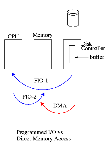
- With or without DMA, the disk controller pulls the desired data
from the disk to its buffer (and pushes data from the buffer to the
disk).
- Without DMA, i.e., with programmed I/O (PIO), the
cpu then does loads and stores (or I/O instructions) to copy the data
from the buffer to the desired memory location.
- With a DMA controller, the controller writes the memory without
intervention of the CPU.
- Clearly DMA saves CPU work. But this might not be important if
the CPU is limited by the memory or by system buses.
- Very important is that there is less data movement so the buses
are used less and the entire operation takes less time.
- Since PIO is pure software it is easier to change, which is an
advantage.
- DMA does need a number of bus transfers from the CPU to the
controller to specify the DMA. So DMA is most effective for large
transfers where the setup is amortized.
- Why have the buffer? Why not just go from the disk straight to
the memory.
Answer: Speed matching. The disk supplies data at a fixed rate, which might
exceed the rate the memory can accept it. In particular the memory
might be busy servicing a request from the processor or from another
DMA controller.
Homework: 12
5.1.5: Interrupts Revisited
Skipped.
5.2: Principles of I/O Software
As with any large software system, good design and layering is
important.
5.2.1: Goals of the I/O Software
Device independence
We want to have most of the OS, unaware of the characteristics of
the specific devices attached to the system. Indeed we also want the
OS to be largely unaware of the CPU type itself.
Due to this device independence, programs are
written to read and write generic devices and then at run time
specific devices are assigned. Writing to a disk has differences from
writing to a terminal, but Unix cp and DOS copy do not see these
differences. Indeed, most of the OS, including the file system code,
is unaware of whether the device is a floppy or hard disk.
Homework: 5.9
Uniform naming
Recall that we discussed the value
of the name space implemented by file systems. There is no dependence
between the name of the file and the device on which it is stored. So
a file called IAmStoredOnAHardDisk might well be stored on a floppy disk.
Error handling
There are several aspects to error handling including: detection,
correction (if possible) and reporting.
- Detection should be done as close to where the error occurred as
possible before more damage is done (fault containment). This is not
trivial.
- Correction is sometimes easy, for example ECC memory does this
automatically (but the OS wants to know about the error so that it can
schedule replacement of the faulty chips before unrecoverable double
errors occur).
Other easy cases include successful retries for failed ethernet
transmissions. In this example, while logging is appropriate, it is
quite reasonable for no action to be taken.
- Error reporting tends to be awful. The trouble is that the error
occurs at a low level but by the time it is reported the
context is lost. Unix/Linux in particular is horrible in this area.
Creating the illusion of synchronous I/O
- I/O must be asynchronous for good performance. That is
the OS cannot simply wait for an I/O to complete. Instead, it
proceeds with other activities and responds to the notification when
the I/O has finished.
- Users (mostly) want no part of this. The code sequence
Read X
Y <-- X+1
Print Y
should print a value one greater than that read. But if the
assignment is performed before the read completes, the wrong value is
assigned.
- Performance junkies sometimes do want the asynchrony so that they
can have another portion of their program executed while the I/O is
underway. That is they implement a mini-scheduler in their
application code.
Buffering
- Often needed to hold data for examination prior to sending it to
its desired destination.
- But this involves copying and takes time.
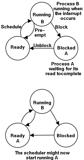
Sharable vs dedicated devices
For devices like printers and tape drives, only one user at a time
is permitted. These are called serially reusable
devices, and were studied in the deadlocks chapter.
Devices like disks and Ethernet ports can be shared by processes
running concurrently.
5.2.2: Programmed I/O
- As mentioned just above, with programmed I/O the
processor moves the data between memory and the device.
- How does the
process know when the device is ready to accept or supply new data?
- In the simplest implementation, the processor loops continually asking
the device. This is called polling or
busy waiting.
- If the device is slow, polling is clearly wasteful, which leads us
to.
5.2.3: Interrupt-Driven I/O
- The device interrupts the processor when it is ready.
- An interrupt service routine then initiates transfer of the next
datum
- Normally better than polling, but not always. Interrupts are
expensive on modern machines.
- To minimize interrupts, better controllers often employ ...
I/O Using DMA
- We discussed DMA above.
- An additional advantage of dma, not mentioned above, is that the
processor is interrupted only at the end of a command not after each
datum is transferred.
- Many devices receive a character at a time, but with a dma
controller, an interrupt occurs only after a buffer has been transferred.
5.3: I/O Software Layers
Layers of abstraction as usual prove to be effective. Most systems
are believed to use the following layers (but for many systems, the OS
code is not available for inspection).
- User level I/O routines.
- Device independent I/O software.
- Device drivers.
- Interrupt handlers.
We will give a bottom up explanation.
5.3.1: Interrupt Handlers
We discussed an interrupt handler before when studying page faults.
Then it was called ``assembly language code''.
In the present case, we have a process blocked on I/O and the I/O
event has just completed. So the goal is to make the process ready.
Possible methods are.
- Releasing a semaphore on which the process is waiting.
- Sending a message to the process.
- Inserting the process table entry onto the ready list.
Once the process is ready, it is up to the scheduler to decide when
it should run.
5.3.2: Device Drivers
The portion of the OS that ``knows'' the characteristics of the
controller.
The driver has two ``parts'' corresponding to its two access
points. Recall the following figure from the beginning of the course.
- Accessed by the main line OS via the envelope in response to an I/O
system call. The portion of the driver accessed in this way is
sometimes call the ``top'' part.
- Accessed by the interrupt handler when the I/O completes (this
completion is signaled by an interrupt). The portion of the driver
accessed in this way is sometimes call the ``bottom'' part.
Tanenbaum describes the actions of the driver assuming it is
implemented as a process (which he recommends). I give both that view
point and the self-service paradigm in which the driver is invoked by
the OS acting in behalf of a user process (more precisely the process
shifts into kernel mode).
Driver in a self-service paradigm
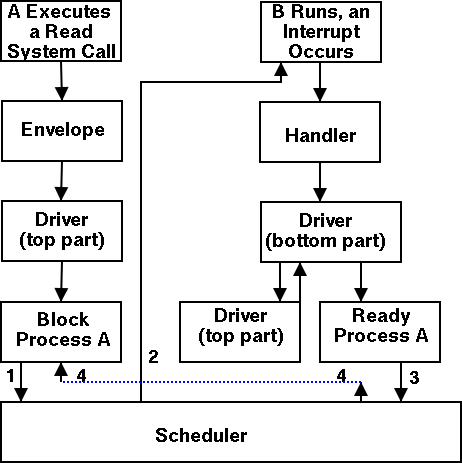
- The user (A) issues an I/O system call.
- The main line, machine independent, OS prepares a
generic request for the driver and calls (the top part of)
the driver.
- If the driver was idle (i.e., the controller was idle), the
driver writes device registers on the controller ending with a
command for the controller to begin the actual I/O.
- If the controller was busy (doing work the driver gave it
previously), the driver simply queues the current request (the
driver dequeues this request below).
- The driver jumps to the scheduler indicating that the current
process should be blocked.
- The scheduler blocks A and runs (say) B.
- B starts running.
- An interrupt arrives (i.e., an I/O has been completed).
- The interrupt handler invokes (the bottom part of) the driver.
- The driver informs the main line perhaps passing data and
surely passing status (error, OK).
- The top part is called to start another I/O if the queue is
nonempty. We know the controller is free. Why?
Answer: We just received an interrupt saying so.
- The driver jumps to the scheduler indicating that process A should
be made ready.
- The scheduler picks a ready process to run. Assume it picks A.
- A resumes in the driver, which returns to the main line, which
returns to the user code.
Driver as a process (Tanenbaum) (less detailed than above)
- The user issues an I/O request. The main line OS prepares a
generic request (e.g. read, not read using Buslogic BT-958 SCSI controller)
for the driver and the driver is awakened (perhaps a message is sent to
the driver to do both jobs).
- The driver wakes up.
- If the driver was idle (i.e., the controller is idle), the
driver writes device registers on the controller ending with a
command for the controller to begin the actual I/O.
- If the controller is busy (doing work the driver gave it), the
driver simply queues the current request (the driver dequeues this
below).
- The driver blocks waiting for an interrupt or for more
requests.
- An interrupt arrives (i.e., an I/O has been completed).
- The driver wakes up.
- The driver informs the main line perhaps passing data and
surely passing status (error, OK).
- The driver finds the next work item or blocks.
- If the queue of requests is non-empty, dequeue one and
proceed as if just received a request from the main line.
- If queue is empty, the driver blocks waiting for an
interrupt or a request from the main line.
5.3.3: Device-Independent I/O Software
The device-independent code does most of the functionality, but not
necessarily most of the code since there can be many drivers
all doing essentially the same thing in slightly different ways due to
slightly different controllers.
- Naming. Again an important O/S functionality.
Must offer a consistent interface to the device drivers.
- In Unix this is done by associating each device with a
(special) file in the /dev directory.
- The i-nodes for these files contain an indication that these
are special files and also contain so called major and minor
device numbers.
- The major device number gives the number of the driver.
(These numbers are rather ad hoc, they correspond to the position
of the function pointer to the driver in a table of function
pointers.)
- The minor number indicates for which device (e.g., which scsi
cdrom drive) the request is intended
- Protection. A wide range of possibilities are
actually done in real systems. Including both extreme examples of
everything is permitted and nothing is permitted (directly).
- In ms-dos any process can write to any file. Presumably, our
offensive nuclear missile launchers do not run dos.
- In IBM and other mainframe OS's, normal processors do not
access devices. Indeed the main CPU doesn't issue the I/O
requests. Instead an I/O channel is used and the mainline
constructs a channel program and tells the channel to invoke it.
- Unix uses normal rwx bits on files in /dev (I don't believe x
is used).
- Buffering is necessary since requests come in a
size specified by the user and data is delivered in a size specified
by the device.
- Enforce exclusive access for non-shared devices
like tapes.
5.3.4: User-Space Software
A good deal of I/O code is actually executed in user space. Some
is in library routines linked into user programs and some is in daemon
processes.
- Some library routines are trivial and just move their arguments
into the correct place (e.g., a specific register) and then issue a
trap to the correct system call to do the real work.
- Some, notably standard I/O (stdio) in Unix, are definitely not
trivial. For example consider the formatting of floating point
numbers done in printf and the reverse operation done in scanf.
- Printing to a local printer is often performed in part by a
regular program (lpr in Unix) and part by a daemon
(lpd in Unix).
The daemon might be started when the system boots or might be started
on demand. I guess it is called a daemon because it is not under the
control of any user. A student has suggested that the usage comes
from the meaning of daemon in Greek mythology, namely a guardian
spirit.
Does anyone know the
reason.
- Printing uses spooling, i.e., the file to be
printed is copied somewhere by lpr and then the daemon works with this
copy. Mail uses a similar technique (but generally it is called
queuing, not spooling).
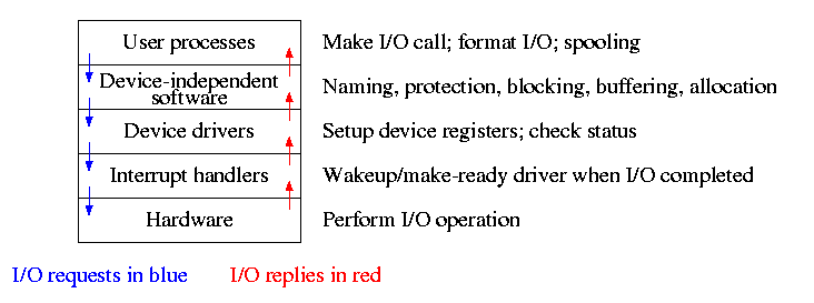
Homework: 10, 13.
5.4: Disks
The ideal storage device is
- Fast
- Big (in capacity)
- Cheap
- Impossible
Disks are big and cheap, but slow.
5.4.1: Disk Hardware
Show a real disk opened up and illustrate the components
- Platter
- Surface
- Head
- Track
- Sector
- Cylinder
- Seek time
- Rotational latency
- Transfer rate
Overlapping I/O operations is important. Many controllers can do
overlapped seeks, i.e. issue a seek to one disk while another is
already seeking.
Modern disks cheat and do not have the
same number of sectors on outer cylinders as on inner one. However,
the disks have electronics and software (firmware) that hides the
cheat and gives the illusion of the same number of sectors on all
cylinders.
(Unofficial) Despite what tanenbaum says later, it is not true that
when one head is reading from cylinder C, all the heads can read from
cylinder C with no penalty. It is, however, true that the penalty is
very small.
Choice of block size
- We discussed this before when studying page size.
- Current commodity disk characteristics (not for laptops) result in
about 15ms to transfer the first byte and 10K bytes per ms for
subsequent bytes (if contiguous).
- Rotation rate is 5400, 7600, or 10,000 RPM (15K just now
available).
- Recall that 6000 RPM is 100 rev/sec or one rev
per 10ms. So half a rev (the average time for to rotate to a
given point) is 5ms.
- Transfer rates around 10MB/sec = 10KB/ms.
- Seek time around 10ms.
- This favors large blocks, 100KB or more.
- But the internal fragmentation would be severe since many files
are small.
- Multiple block sizes have been tried as have techniques to try to
have consecutive blocks of a given file near each other.
- Typical block sizes are 4KB-8KB.
Homework:
Consider a disk with an average seek time of 10ms, an average
rotational latency of 5ms, and a transfer rate of 10MB/sec.
- If the block size is 1KB, how long would it take to read a block?
- If the block size is 100KB, how long would it take to read a
block?
- If the goal is to read 1K, a 1KB block size is better as the
remaining 99KB are wasted. If the goal is to read 100KB, the 100KB
block size is better since the 1KB block size needs 100 seeks and 100
rotational latencies. What is the minimum size request for which a
disk with a 100KB block size would complete faster than one with a 1KB
block size?
RAID (Redundant Array of Inexpensive Disks) (Skipped)
- The name RAID is from Berkeley.
- IBM changed the name to Redundant Array of Independent
Disks. I wonder why?
- A simple form is mirroring, where two disks contain the
same data.
- Another simple form is striping (interleaving) where consecutive
blocks are spread across multiple disks. This helps bandwidth, but is
not redundant. Thus it shouldn't be called RAID, but it sometimes is.
- One of the normal RAID methods is to have N (say 4) data disks and one
parity disk. Data is striped across the data disks and the bitwise
parity of these sectors is written in the corresponding sector of the
parity disk.
- On a read if the block is bad (e.g., if the entire disk is bad or
even missing), the system automatically reads the other blocks in the
stripe and the parity block in the stripe. Then the missing block is
just the bitwise exclusive or of all these blocks.
- For reads this is very good. The failure free case has no penalty
(beyond the space overhead of the parity disk). The error case
requires N+1 (say 5) reads.
- A serious concern is the small write problem. Writing a sector
requires 4 I/O. Read the old data sector, compute the change, read
the parity, compute the new parity, write the new parity and the new
data sector. Hence one sector I/O became 4, which is a 300% penalty.
- Writing a full stripe is not bad. Compute the parity of the N
(say 4) data sectors to be written and then write the data sectors and
the parity sector. Thus 4 sector I/Os become 5, which is only a 25%
penalty and is smaller for larger N, i.e., larger stripes.
- A variation is to rotate the parity. That is, for some stripes
disk 1 has the parity, for others disk 2, etc. The purpose is to not
have a single parity disk since that disk is needed for all small
writes and could become a point of contention.
5.4.2: Disk Formatting
Skipped.
5.4.3: Disk Arm Scheduling Algorithms
There are three components to disk response time: seek, rotational
latency, and transfer time. Disk arm scheduling is concerned with
minimizing seek time by reordering the requests.
These algorithms are relevant only if there are several I/O
requests pending. For many PCs this is not the case. For most
commercial applications, I/O is crucial and there are often many
requests pending.
- FCFS (First Come First Served): Simple but has long delays.
- Pick: Same as FCFS but pick up requests for cylinders that are
passed on the way to the next FCFS request.
- SSTF or SSF (Shortest Seek (Time) First): Greedy algorithm. Can
starve requests for outer cylinders and almost always favors middle
requests.
- Scan (Look, Elevator): The method used by an old fashioned
jukebox (remember ``Happy Days'') and by elevators. The disk arm
proceeds in one direction picking up all requests until there are no
more requests in this direction at which point it goes back the other
direction. This favors requests in the middle, but can't starve any
requests.
- C-Scan (C-look, Circular Scan/Look): Similar to Scan but only
service requests when moving in one direction. When going in the
other direction, go directly to the furthest away request. This
doesn't favor any spot on the disk. Indeed, it treats the cylinders
as though they were a clock, i.e. after the highest numbered cylinder
comes cylinder 0.
- N-step Scan: This is what the natural implementation of Scan
gives.
- While the disk is servicing a Scan direction, the controller
gathers up new requests and sorts them.
- At the end of the current sweep, the new list becomes the next
sweep.
Minimizing Rotational Latency
Use Scan based on sector numbers not cylinder number. For
rotational latency Scan which is the same as C-Scan. Why?
Ans: Because the disk only rotates in one direction.
Homework: 24, 25
5.4.4: Error Handling
Disks error rates have dropped in recent years. Moreover, bad
block forwarding is normally done by the controller (or disk electronic) so
this topic is no longer as important for OS.
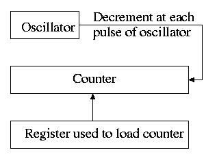
5.5: Clocks
Also called timers.
5.5.1: Clock Hardware
- Generates an interrupt when timer goes to zero
- Counter reload can be automatic or under software (OS) control.
- If done automatically, the interrupt occurs periodically and thus
is perfect for generating a clock interrupt at a fixed period.
5.5.2: Clock Software
- TOD: Bump a counter each tick (clock interupt). If counter is
only 32 bits must worry about overflow so keep two counters: low order
and high order.
- Time quantum for RR: Decrement a counter at each tick. The quantum
expires when counter is zero. Load this counter when the scheduler
runs a process.
- Accounting: At each tick, bump a counter in the process table
entry for the currently running process.
- Alarm system call and system alarms:
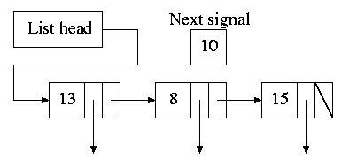
- Users can request an alarm at some future time.
- The system also on occasion needs to schedule some of its own
activities to occur at specific times in the future (e.g. turn off
the floppy motor).
- The conceptually simplest solution is to have one timer for
each event.
- Instead, we simulate many timers with just one.
- The data structure on the right works well.
- The time in each list entry is the time after the
preceding entry that this entry's alarm is to ring.
- For example, if the time is zero, this event occurs at the
same time as the previous event.
- The other entry is a pointer to the action to perform.
- At each tick, decrement next-signal.
- When next-signal goes to zero,
process the first entry on the list and any others following
immediately after with a time of zero (which means they are to be
simultaneous with this alarm). Then set next-signal to the value
in the next alarm.
- Profiling
- Want a histogram giving how much time was spent in each 1KB
(say) block of code.
- At each tick check the PC and bump the appropriate counter.
- A user-mode program can determine the software module
associated with each 1K block.
- If we use finer granularity (say 10B instead of 1KB), we get
increased accuracy but more memory overhead.
Homework: 27
5.6: Character-Oriented Terminals
5.6.1: RS-232 Terminal Hardware
Quite dated. It is true that modern systems can communicate to a
hardwired ascii terminal, but most don't. Serial ports are used, but
they are normally connected to modems and then some protocol (SLIP,
PPP) is used not just a stream of ascii characters. So skip this
section.
Memory-Mapped Terminals
Not as dated as the previous section but it still discusses the
character not graphics interface.
- Today, software writes into video memory
the bits that are to be put on the screen and then the graphics
controller
converts these bits to analog signals for the monitor (actually laptop
displays and some modern monitors are digital).
- But it is much more complicated than this. The graphics
controllers can do a great deal of video themselves (like filling).
- This is a subject that would take many lectures to do well.
- I believe some of this is covered in 201.
Keyboards
Tanenbaum description of keyboards is correct.
- At each key press and key release a code is written into the
keyboard controller and the computer is interrupted.
- By remembering which keys have been depressed and not released
the software can determine Cntl-A, Shift-B, etc.
5.6.2: Input Software
- We are just looking at keyboard input. Once again graphics is too
involved to be treated here.
- There are two fundamental modes of input, sometimes called
raw and cooked.
- In raw mode the application sees every ``character'' the user
types. Indeed, raw mode is character oriented.
- All the OS does is convert the keyboard ``scan codes'' to
``characters'' and and pass these characters to the application.
- Some examples
- down-cntl down-x up-x up-cntl is converted to cntl-x
- down-cntl up-cntl down-x up-x is converted to x
- down-cntl down-x up-cntl up-x is converted to cntl-x (I just
tried it to be sure).
- down-x down-cntl up-x up-cntl is converted to x
- Full screen editors use this mode.
- Cooked mode is line oriented. The OS delivers lines to the
application program.
- Special characters are interpreted as editing characters
(erase-previous-character, erase-previous-word, kill-line, etc).
- Erased characters are not seen by the application but are
erased by the keyboard driver.
- Need an escape character so that the editing characters can be
passed to the application if desired.
- The cooked characters must be echoed (what should one do if the
application is also generating output at this time?)
- The (possibly cooked) characters must be buffered until the
application issues a read (and an end-of-line EOL has been received
for cooked mode).
5.6.3: Output Software
Again too dated and the truth is too complicated to deal with in a
few minutes.
5.7: Graphical User Interfaces (GUIs)
Skipped.
5.8: Network Terminals
Skipped.
5.9: Power Management
Skipped.
5.10: Research on Input/Output
Skipped.
5.11: Summary
Read.
================ Start Lecture #14 ================
Chapter 6: File Systems
Requirements
- Size: Store very large amounts of data.
- Persistence: Data survives the creating process.
- Access: Multiple processes can access the data concurrently.
Solution: Store data in files that together form a file system.
6.1: Files
6.1.1: File Naming
Very important. A major function of the file system.
- Does each file have a unique name?
Answer: Often no. We will discuss this below when we study
links.
- Extensions, e.g. the ``html'' in ``class-notes.html''.
- Conventions just for humans: letter.teq (my convention).
- Conventions giving default behavior for some programs.
- The emacs editor thinks .html files should be edited in
html mode but
can edit them in any mode and can edit any file
in html mode.
- Netscape thinks .html means an html file, but
<html> ... </html> works as well
- Gzip thinks .gz means a compressed file but accepts a
--suffix flag
- Default behavior for Operating system or window manager or
desktop environment.
- Click on .xls file in windows and excel is started.
- Click on .xls file in nautilus under linux and gnumeric is
started.
- Required extensions for programs
- The gnu C compiler (and probably others) requires C
programs be named *.c and assembler programs be named *.s
- Required extensions by operating systems
- MS-DOS treats .com files specially
- Windows 95 requires (as far as I can tell) shortcuts to
end in .lnk.
- Case sensitive?
Unix: yes. Windows: no.
6.1.2: File structure
A file is a
- Byte stream
- Unix, dos, windows (I think).
- Maximum flexibility.
- Minimum structure.
- (fixed size) Record stream: Out of date
- 80-character records for card images.
- 133-character records for line printer files. Column 1 was
for control (e.g., new page) Remaining 132 characters were printed.
- Varied and complicated beast.
- Indexed sequential.
- B-trees.
- Supports rapidly finding a record with a specific
key.
- Supports retrieving (varying size) records in key order.
- Treated in depth in database courses.
Remark: In spring 2002, due to my attending a
conference, showing all the parts of a disk and doing a problem
involving I/O time are done here.
6.1.3: File types
Examples
- (Regular) files.
- Directories: studied below.
- Special files (for devices).
Uses the naming power of files to unify many actions.
    dir             # prints on screen
    dir > file      # result put in a file
    dir > /dev/tape # results written to tape
- ``Symbolic'' Links (similar to ``shortcuts''): Also studied
below.
``Magic number'': Identifies an executable file.
- There can be
several different magic numbers for different types of
executables.
- unix: #!/usr/bin/perl
Strongly typed files:
- The type of the file determines what you can do with the
file.
- This make the easy and (hopefully) common case easier and, more
importantly safer.
- It tends to make the unusual case harder. For example, you have a
program that turns out data (.dat) files. But you want to use it to
turn out a java file but the type of the output is data and cannot be
easily converted to type java.
6.1.4: File access
There are basically two possibilities, sequential access and random
access (a.k.a. direct access).
Previously, files were declared to be sequential or random.
Modern systems do not do this.
Instead all files are random and optimizations are applied when the
system dynamically determines that a file is (probably) being accessed
sequentially.
- With Sequential access the bytes (or records)
are accessed in order (i.e., n-1, n, n+1, ...).
Sequential access is the most common and
gives the highest performance.
For some devices (e.g. tapes) access ``must'' be sequential.
- With random access, the bytes are accessed in any
order. Thus each access must specify which bytes are desired.
6.1.5: File attributes
A laundry list of properties that can be specified for a file
For example:
- hidden
- do not dump
- owner
- key length (for keyed files)
6.1.6: File operations
- Create:
Essential if a system is to add files. Need not be a separate system
call (can be merged with open).
- Delete:
Essential if a system is to delete files.
- Open:
Not essential. An optimization in which the translation from file name to
disk locations is perform only once per file rather than once per access.
- Close:
Not essential. Free resources.
- Read:
Essential. Must specify filename, file location, number of bytes,
and a buffer into which the data is to be placed.
Several of these parameters can be set by other
system calls and in many OS's they are.
- Write:
Essential if updates are to be supported. See read for parameters.
- Seek:
Not essential (could be in read/write). Specify the
offset of the next (read or write) access to this file.
- Get attributes:
Essential if attributes are to be used.
- Set attributes:
Essential if attributes are to be user settable.
- Rename:
Tanenbaum has strange words. Copy and delete is not acceptable for
big files. Moreover copy-delete is not atomic. Indeed link-delete is
not atomic so even if link (discussed below)
is provided, renaming a file adds functionality.
Homework: 6, 7.
6.1.7: An Example Program Using File System Calls
Homework: Read and understand ``copyfile''.
Notes on copyfile
- Normally in unix one wouldn't call read and write directly.
- Indeed, for copyfile, getchar() and putchar() would be nice since
they take care of the buffering (standard I/O, stdio).
- If you compare copyfile from the 1st to 2nd edition, you can see
the addition of error checks.
6.1.8: Memory mapped files (Unofficial)
Conceptually simple and elegant. Associate a segment with each
file and then normal memory operations take the place of I/O.
Thus copyfile does not have fgetc/fputc (or read/write). Instead it is
just like memcopy
while ( *(dest++) = *(src++) );
The implementation is via segmentation with demand paging but
the backing store for the pages is the file itself.
This all sounds great but ...
- How do you tell the length of a newly created file? You know
which pages were written but not what words in those pages. So a file
with one byte or 10, looks like a page.
- What if same file is accessed by both I/O and memory mapping.
- What if the file is bigger than the size of virtual memory (will
not be a problem for systems built 3 years from now as all will have
enormous virtual memory sizes).
6.2: Directories
Unit of organization.
6.2.1-6.2.3: Single-level, Two-level, and Hierarchical directory systems
Possibilities
- One directory in the system (Single-level)
- One per user and a root above these (Two-level)
- One tree
- One tree per user
- One forest
- One forest per user
These are not as wildly different as they sound.
- If the system only has one directory, but allows the character / in
a file name. Then one could fake a tree by having a file named
/allan/gottlieb/courses/arch/class-notes.html
rather than a directory allan, a subdirectory gottlieb, ..., a file
class-notes.html.
- Dos (windows) is a forest, unix a tree. In dos there is no common
parent of a:\ and c:\.
- But windows explorer makes the dos forest look quite a bit like a
tree. Indeed, the original gnome file manager for linux, looks A LOT
like windows explorer.
- You can get an effect similar to (but not the same as) one X per
user by having just one X in the system and having permissions that
permits each user to visit only a subset. Of course if the system
doesn't have permissions, this is not possible.
- Today's systems have a tree per system or a forest per system.
6.2.4: Path Names
You can specify the location of a file in the file hierarchy by
using either an absolute or a
Relative path to the file
- An absolute path starts at the (or ``one of the'', if we have a
forest) root(s).
- A relative path starts at the
current (a.k.a working) directory.
- The special directories . and .. represent the current directory
and the parent of the current directory respectively.
Homework: 1, 9.
6.2.5: Directory operations
- Create: Produces an ``empty'' directory.
Normally the directory created actually contains . and .., so is not
really empty
- Delete: Requires the directory to be empty (i.e., to just contain
. and ..). Commands are normally written that will first empty the
directory (except for . and ..) and then delete it. These commands
make use of file and directory delete system calls.
- Opendir: Same as for files (creates a ``handle'')
- Closedir: Same as for files
- Readdir: In the old days (of unix) one could read directories as files
so there was no special readdir (or opendir/closedir). It was
believed that the uniform treatment would make programming (or at
least system understanding) easier as there was less to learn.
However, experience has taught that this was not a good idea since
the structure of directories then becomes exposed. Early unix had a
simple structure (and there was only one). Modern systems have more
sophisticated structures and more importantly they are not fixed
across implementations.
- Rename: As with files
- Link: Add a second name for a file; discussed
below.
- Unlink: Remove a directory entry. This is how a file is deleted.
But if there are many links and just one is unlinked, the file
remains. Discussed in more
detail below.
6.3: File System Implementation
6.3.1: File System Layout
- One disk starts with a Master Boot Record (MBR).
- Each disk has a partition table.
- Each partition holds one file system.
- Each partition typically contains some parameters (e.g., size),
free blocks, and blocks in use. The details vary.
- In unix some of the in use blocks contains I-nodes each of which
describes a file or directory and is described below.
- During boot the MBR is read and executed. It transfers control to
the boot block of the active partition.
6.3.2: Implementing Files
- A disk cannot read or write a single word. Instead it can read or
write a sector, which is often 512 bytes.
- Disks are written in blocks whose size is a multiple of the sector
size.
Contiguous allocation
- This is like OS/MVT.
- The entire file is stored as one piece.
- Simple and fast for access, but ...
- Problem with growing files
- Must either evict the file itself or the file it is bumping
into.
- Same problem with an OS/MVT kind of system if jobs grow.
- Problem with external fragmentation.
- No longer used for general purpose rewritable file systems.
- Ideal for file systems where files do not change size.
- Used for CD-ROM file systems.
Homework: 12.
Linked allocation
- The directory entry contains a pointer to the first block of the file.
- Each block contains a pointer to the next.
- Horrible for random access.
- Not used.
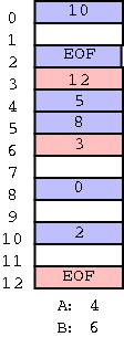
FAT (file allocation table)
- Used by dos and windows (but not windows/NT).
- Directory entry points to first block (i.e. specifies the block
number).
- A FAT is maintained in memory having one (word) entry for each
disk block. The entry for block N contains the block number of the
next block in the same file as N.
- This is linked but the links are stored separately.
- Time to access a random block is still is linear in size of file
but now all the references are to this one table which is in memory.
So it is bad but not horrible for random access.
- Size of table is one word per disk block. If blocks are of size
4K and the FAT uses 4-byte words, the table is one megabyte for
each disk gigabyte. Large but perhaps not prohibitive.
- If blocks are of size 512 bytes (the sector size of most disks)
then the table is 8 megs per gig, which is probably prohibitive.
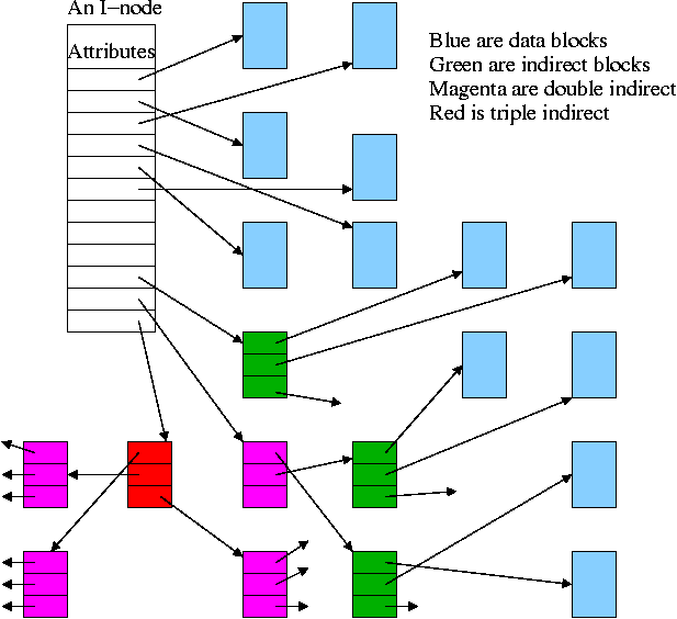
I-Nodes
- Used by unix/linux.
- Directory entry points to i-node (index-node).
- I-Node points to first few data blocks, often called direct blocks.
- I-Node also points to an indirect block, which points to disk blocks.
- I-Node also points to a double indirect, which points an indirect ...
- For some implementations there are triple indirect as well.
- The i-node is in memory for open files.
So references to direct blocks take just one I/O.
- For big files most references require two I/Os (indirect + data).
- For huge files most references require three I/Os (double
indirect, indirect, and data).
6.3.3: Implementing Directories
Recall that a directory is a mapping that converts file (or
subdirectory) names to the files (or subdirectories) themselves.
Trivial File System (CP/M)
- Only one directory in the system.
- Directory entry contains pointers to disk blocks.
- If need more blocks, get another directory entry.
MS-DOS and Windows (FAT)
- Subdirectories supported.
- Directory entry contains metatdata such as date and size
as well as pointer to first block.
- The FAT has the pointers to the remaining blocks.
Unix/linux
- Each entry contains a name and a pointer to the corresponding i-node.
- Metadata is in the i-node.
- Early unix had limit of 14 character names.
- Name field now is varying length.
- To go down a level in directory takes two steps: get i-node, get
file (or subdirectory).
- Do on the blackboard the steps for
/allan/gottlieb/courses/os/class-notes.html
Homework: 27
6.3.4: Shared files (links)
- ``Shared'' files is Tanenbaum's terminology.
- More descriptive would be ``multinamed files''.
- If a file exists, one can create another name for it (quite
possibly in another directory).
- This is often called creating a (or another) link to the file.
- Unix has two flavor of links, hard links and
symbolic links or symlinks.
- Dos/windows has symlinks, but I don't believe it has hard links.
- These links often cause confusion, but I really believe that the
diagrams I created make it all clear.
Hard Links
- Symmetric multinamed files.
- When a hard like is created another name is created for
the same file.
- The two names have equal status.
- It is not, I repeat NOT, true that one
name is the ``real name'' and the other one is ``just a link''.
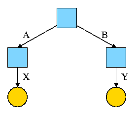
Start with an empty file system (i.e., just the root directory) and
then execute:
cd /
mkdir /A; mkdir /B
touch /A/X; touch /B/Y
We have the situation shown on the right.
- Circles represent ordinary files.
- Squares represent directories.
- One name for the left circle is /A/X.
- I have written the names on the edges.
- This is not customary, normally they are written in the
circles or squares.
- When there are no multi-named files, it doesn't matter if they
are written in the node or edge.
- We will see that when files can have multiple names it is much
better to write the name on the edge.
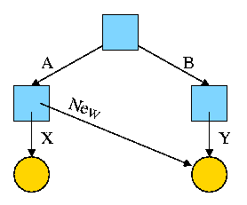 Now execute
ln /B/Y /A/New
This gives the new diagram to the right.
At this point there are two equally valid name for the right hand
yellow file, /B/Y and /A/New. The fact that /B/Y was created first is
NOT detectable.
- Both point to the same i-node.
- Only one owner (the one who created the file initially).
- One date, one set of permissions, one ... .
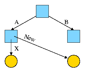
Assume Bob created /B and /B/Y and Alice created /A, /A/X, and /A/New.
Later Bob tires of /B/Y and removes it by executing
rm /B/Y
The file /A/New is still fine (see third diagram on the right).
But it is owned by Bob, who can't find it! If the system enforces
quotas bob will likely be charged (as the owner), but he can neither
find nor delete the file (since bob cannot unlink, i.e. remove, files
from /A)
Since hard links are only permitted to files (not directories) the
resulting file system is a dag (directed acyclic graph). That is, there
are no directed cycles. We will now proceed to give away this useful
property by studying symlinks, which can point to directories.
Symlinks
- Asymmetric multinamed files.
- When a symlink is created another file is created.
The contents of the new file is the name
of the original file.
- A hard link in contrast points to the original
file.
- he examples will make this clear.
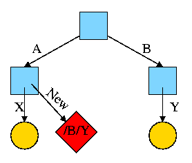
Again start with an empty file system and this time execute
cd /
mkdir /A; mkdir /B
touch /A/X; touch /B/Y
ln -s /B/Y /A/New
We now have an additional file /A/New, which is a symlink to /B/Y.
- The file named /A/New has the name /B/Y as its data
(not metadata).
- The system notices that A/New is a diamond (symlink) so reading
/A/New will return the contents of /B/Y (assuming the reader has read
permission for /B/Y).
- If /B/Y is removed /A/New becomes invalid.
- If a new /B/Y is created, A/New is once again valid.
- Removing /A/New has no effect of /B/Y.
- If a user has write permission for /B/Y, then writing /A/New is possible
and writes /B/Y.
The bottom line is that, with a hard link, a new name is created
for the file.
This new name has equal status with the original name.
This can cause some
surprises (e.g., you create a link but I own the file).
With a symbolic link a new file is created (owned by the
creator naturally) that contains the name of the original file.
We often say the new file points to the original file.
Question: Consider the hard link setup above. If Bob removes /B/Y
and then creates another /B/Y, what happens to /A/New?
Answer: Nothing. /A/New is still a file with the same contents as the
original /B/Y.
Question: What about with a symlink?
Answer: /A/New becomes invalid and then valid again, this time pointing
to the new /B/Y.
(It can't point to the old /B/Y as that is completely gone.)
Note:
Shortcuts in windows contain more that symlinks in unix. In addition
to the file name of the original file, they can contain arguments to
pass to the file if it is executable. So a shortcut to
netscape.exe
can specify
netscape.exe //allan.ultra.nyu.edu/~gottlieb/courses/os/class-notes.html
End of Note
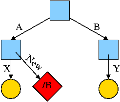
What about symlinking a directory?
cd /
mkdir /A; mkdir /B
touch /A/X; touch /B/Y
ln -s /B /A/New
Is there a file named /A/New/Y ?
Yes.
What happens if you execute cd /A/New/.. ?
- Answer: Not clear!
- Clearly you are changing directory to the parent directory of
/A/New. But is that /A or /?
- The command interpreter I use offers both possibilities.
- cd -L /A/New/.. takes you to A (L for logical).
- cd -P /A/New/.. takes you to / (P for physical).
- cd /A/New/.. takes you to A (logical is the default).
What did I mean when I said the pictures made it all clear?
Answer: From the file system perspective it is clear.
It is not always so clear what programs will do.
6.3.5: Disk space management
All general purpose systems use a (non-demand) paging
algorithm for file storage. Files are broken into fixed size pieces,
called blocks that can be scattered over the disk.
Note that although this is paging, it is never called paging.
The file is completely stored on the disk, i.e., it is not
demand paging.
Actually, it is more complicated
- Various optimizations are
performed to try to have consecutive blocks of a single file stored
consecutively on the disk. Discussed
below
.
- One can imagine systems that store only parts of the file on disk
with the rest on tertiary storage (some kind of tape).
- This would be just like demand paging.
- Perhaps NASA does this with their huge datasets.
- Caching (as done for example in microprocessors) is also the same
as demand paging.
- We unify these concepts in the computer architecture course.
Choice of block size
- We discussed this before when studying page size.
- Current commodity disk characteristics (not for laptops) result in
about 15ms to transfer the first byte and 10K bytes per ms for
subsequent bytes (if contiguous).
- This was explained in the I/O chapter.
- Rotation rate is 5400, 7600, or 10,000 RPM (15K is now
available).
- Recall that 6000 RPM is 100 rev/sec or one rev
per 10ms. So half a rev (the average time for to rotate to a
given point) is 5ms.
- Transfer rates around 10MB/sec = 10KB/ms.
- Seek time is around 10ms.
- This favors large blocks, 100KB or more.
- But the internal fragmentation would be severe since many files
are small.
- Typical block sizes are 4KB and 8KB.
- Unofficial
- Systems that contain multiple block sizes have been tried
(i.e., the system uses blocks of size A for some files and blocks
of size B for other files).
- Some systems use techniques to try to have consecutive blocks
of a given file near each other as well as blocks of ``related''
files (e.g., files in the same directory).
Storing free blocks
There are basically two possibilities
- An in-memory bit map.
- One bit per block
- If block size is 4KB = 32K bits, 1 bit per 32K bits
- So 32GB disk (potentially all free) needs 1MB ram.
- Variation is to demand page the bit map. This saves space
(RAM) at the cost of I/O.
- Linked list with each free block pointing to next.
- Thus you must do a read for each request.
- But reading a free block is a wasted I/O.
- Instead some free blocks contain pointers to other free
blocks. This has much less wasted I/O, but is more complicated.
- When read a block of pointers store them in memory.
- See diagram on right.
6.3.6: File System reliability
Bad blocks on disks
Not so much of a problem now. Disks are more reliable and, more
importantly, disks take care of the bad blocks themselves. That is,
there is no OS support needed to map out bad blocks. But if a block
goes bad, the data is lost (not always).
Backups
All modern systems support full and
incremental dumps.
- A level 0 dump is a called a full dump (i.e., dumps everything).
- A level n dump (n>0) is called an incremental dump and the
standard unix utility dumps
all files that have changed since the previous level n-1 dump.
- Other dump utilities dump all files that have changed since the
last level n dump.
- Keep on the disk the dates of the most recent level i dumps
for all i. In Unix this is traditionally in /etc/dumpdates.
- What about the nodump attribute?
- Default policy (for Linux at least) is to dump such files
anyway when doing a full dump, but not dump them for incremental
dumps.
- Another way to say this is the nodump attribute is honored for
level n dumps if n>1.
- The dump command has an option to override the default policy
(can specify k so that nodump is honored for level n dumps if n>k).
Consistency
- Fsck (file system check) and chkdsk (check disk)
- If the system crashed, it is possible that not all metadata was
written to disk. As a result the file system may be inconsistent.
These programs check, and often correct, inconsistencies.
- Scan all i-nodes (or fat) to check that each block is in exactly
one file, or on the free list, but not both.
- Also check that the number of links to each file (part of the
metadata in the file's i-node) is correct (by
looking at all directories).
- Other checks as well.
- Offers to ``fix'' the errors found (for most errors).
- ``Journaling'' file systems
- An idea from database theory (transaction logs).
- Vastly reduces the need for fsck.
- NTFS has had journaling from day 1.
- Many Unix systems have it. IBM's AIX converted to journaling
in the early 90s.
- Linux distributions now have journaling (2001-2002).
- FAT does not have journaling.
6.3.7 File System Performance
Buffer cache or block cache
An in-memory cache of disk blocks.
- Demand paging again!
- Clearly good for reads as it is much faster to read memory than to
read a disk.
- What about writes?
- Must update the buffer cache (otherwise subsequent reads will
return the old value).
- The major question is whether the system should also update
the disk block.
- The simplest alternative is write through
in which each write is performed at the disk before it declared
complete.
- Since floppy disk drivers adopt a write through policy,
one can remove a floppy as soon as an operation is complete.
- Write through results in heavy I/O write traffic.
- If a block is written many times all the writes are
sent the disk. Only the last one was ``needed''.
- If a temporary file is created, written, read, and
deleted, all the disk writes were wasted.
- DOS uses write-through
- The other alternative is write back in which
the disk is not updated until the in-memory copy is
evicted (i.e., at replacement time).
- Much less write traffic than write through.
- Trouble if a crash occurs.
- Used by Unix and others for hard disks.
- Can write dirty blocks periodically, say every minute.
This limits the possible damage, but also the possible gain.
- Ordered writes. Do not write a block containing pointers
until the block pointed to has been written. Especially if
the block pointed to contains pointers since the version of
these pointers on disk may be wrong and you are giving a file
pointers to some random blocks.--unofficial for 202
Homework: 29.
Block Read Ahead
When the access pattern ``looks'' sequential read ahead is employed.
This means that after completing a read() request for block n of a file.
The system guesses that a read() request for block n+1 will shortly be
issued so it automatically fetches block n+1.
- How do you decide that the access pattern looks sequential?
- If a seek system call is issued, the access pattern is not
sequential.
- If a process issues consecutive read() system calls for block
n-1 and then n, the access patters is
guessed to be sequential.
- What if block n+1 is already in the block cache?
Ans: Don't issue the read ahead.
- Would it be reasonable to read ahead two or three blocks?
Ans: Yes.
- Would it be reasonable to read ahead the entire file?
Ans: No, it could easily pollute the cache evicting needed blocks and
could waste considerable disk bandwidth.
Reducing Disk Arm Motion
Try to place near each other blocks that are going to be read in
succession.
- If the system uses a bitmap for the free list, it can
allocate a new block for a file close to the previous block
(guessing that the file will be accessed sequentially).
- The system can perform allocations in ``super-blocks'', consisting
of several contiguous blocks.
- Block cache and I/O requests are still in blocks.
- If the file is accessed sequentially, consecutive blocks of a
super-block will be accessed in sequence and these are
contiguous on the disk.
- For a unix-like file system, the i-nodes can be placed in the
middle of the disk, instead of at one end, to reduce the seek time
to access an i-node followed by a block of the file.
- Can divide the disk into cylinder groups, each
of which is a consecutive group of cylinders.
- Each cylinder group has its own free list and, for a unix-like
file system, its own space for i-nodes.
- If possible, the blocks for a file are allocated in the same
cylinder group as is the i-node.
- This reduces seek time if consecutive accesses are for the
same file.
6.3.8: Log-Structured File Systems (unofficial)
A research file system that tries to make all writes sequential.
That is, writes are treated as if going to a log file.
This project worked with a unix-like file system, i.e. was i-node based.
- Assumption is that large block caches will eliminate most disk
reads so we need to improve writes.
- Buffer writes until have (say) 1MB to write.
- When the buffer is full, write it to the end of the disk (treating
the disk as a log).
- Thus writes are sequential and hence fast
- The 1MB units on the disk are called (unfortunately) segments.
I will refer to the buffer as the segment buffer.
- A segment can have i-nodes, direct blocks, indirect blocks,
blocks forming part of a file, blocks forming part of a directory.
In short a segment contains the most recently modified (or
created) 1MB of blocks.
- Note that modified blocks are not reclaimed!
- The system keeps a map of where the most recent version of each
i-node is located. The map is on disk (but the heavily accessed
parts will be in the block cache.
- So the (most up to date) i-node of a file can be found and from
that the entire file can be found.
- But the disk will fill with garbage since modified blocks are not
reclaimed.
- A ``cleaner'' process runs in the background and examines
segments starting from the beginning.
It removes overwritten blocks and then adds the remaining blocks
to the segment buffer. (This is not trivial.)
- Thus the disk is compacted and is treated like a circular array of
segments.
6.4: Example File Systems (watch this space)
6.4.1: CD-ROM File Systems (skipped)
6.4.2: The CP/M File System
This was done above.
6.4.3: The MS-DOS File System
This was done above.
6.4.4: The windows 98 File System
Two changes were made: Long file names were supported and the
allocation table was switched from FAT-16 to FAT-32.
-
The only hard part was to keep compatibility with the old 8.3
naming rule. This is called ``backwards compatibility''.
A file has two name a long one and an 8.3. If the long name fits
the 8.3 format, only one name is kept. If the long name does not
fit the 8+3, an 8+3 version is produce via an algorithm, that
works but the names produced are not lovely.
-
FAT-32 used 32 bit words for the block numbers so the fat table
could be huge. Windows 98 kept only a portion of the FAT-32 table
in memory at a time. (I do not know the replacement policy,
number of blocks kept in memory, etc).
6.4.5: The Unix V7 File System
This was done above.
Draw the steps to find /allan/gottlieb/linker.java
6.5: Research on File Systems (skipped)
6.6 Summary (read)
The End: Good luck on the final