Basic Algorithms

Chapter 5 Fundamental Techniques

5.1 The Greedy Method

The greedy method is applied to maximization/minimization problems. The idea is to at each decision point choose the configuration that maximizes/minimizes the objective function so far. Clearly this does not lead to the global max/min for all problems, but it does for a number of problems.

This chapter does not make a good case for the greedy method. since it is used to solve simple cases of standard problems in which the more normal cases do not use the greedy method. However, there are better examples, for example minimal the spanning tree and shortest path graph problems. The two algorithms chosen for this section, fractional knapsack and task scheduling, were (presumably) chosen because they are simple and natural to solve with the greedy method.

5.1.1 The Fractional Knapsack Method

In the knapsack problem we have a knapsack of a fixed capacity (say W pounds) and different items i each with a given weight wi and a given benefit bi. We want to put items into the knapsack so as to maximize the benefit subject to the constraint that the sum of the weights must be less than W.

The knapsack problem is actually rather difficult in the normal case where one must either put an item in the knapsack or not. However, in this section, in order to illustrate greedy algorithms, we consider a much simpler variation in which we can take part of an item and get a proportional part of the benefit. This is called the ``fractional knapsack problem'' since we can take a fraction of an item. (The more common knapsack problem is called the ``0-1 knapsack problem'' since we either take all (1) or none (0) of an item.

In symbols, for each item i we choose an amount xi (0≤xi≤wi) that we will place in the knapsack. We are subject to the constraint that the sum of the xi is no more than W since that is all the knapsack can hold.

We again desire to maximize the total benefit. Since, for item i, we only put xi in the knapsack, we don't get the full benefit. Specifically we get benefit (xi/wi)bi.

But now this is easy!

• Item i has benefit bi and weighs wi.
• So its value (per pound) is vi=bi/wi.
• We make the greedy choice and pick the most valuable item and take all of it or as much as the knapsack can hold.
• Then we move to the second most valuable and do the same.
• This clearly is optimal since it never makes sense to leave over some valuable item to take some less valuable item.

Why doesn't this work for the normal knapsack problem when we must take all of an item or none of it?

• Example: W=6, w1=4, w2=w3=3, b1=5, b2=b3=3.
• So v1=5/4, v2=v3=1
• Start with the most valuable item, number 1 and put it n the knapsack.
• Knapsack can hold 7-4=2 more "pounds" but remaining items won't fit
• So the total benefit carried is 5.
• The right solution is to take items 2 and 3 for a total benefit of 6.
• The difference between this item and fractional knapsack is that the knapsack can still hold 2/3 of item 2, but we can't take part of an item as we can in the fractional knapsack problem.

Algorithm

algorithm FractionalKnapsack(S,W):
   Input:  Set S of items i with weight wi and benefit bi all positive.
           Knapsack capacity W>0.
   Output: Amount xi of i that maximizes the total benefit without
           exceeding the capacity.

   for each i in S do
      xi ← 0        { for items not chosen in next phase }
      vi ← bi/wi    { the value of item i "per pound" }
   w ← W            { remaining capacity in knapsack }

   while w > 0 do
      remove from S an item of maximal value   { greedy choice }
      xi ← min(wi,w)  { can't carry more than w more }
      w ← w-xi

Analysis

FractionalKnapsack has time complexity O(NlogN) where N is the number of items in S.

• The book suggests assuming S is a heap-based priority queue and then the removal has complexity Θ(logN) so the up to N removals take O(NlogN). The rest of the algorithm is O(N).
• Alternatively, S could be a sequence and we could begin FractionalKnapsack by sorting S with a Θ(NlogN) sort. Now the removal is simply removing the first element. If we use a circular list for S, the removal is O(1) so the algorithm is O(N). Including the sort we again have O(NlogN).

Homework: R-5.1

5.1.2 Task Scheduling

We again consider an easy case of a well known optimization problem.

• We have a set T of N tasks, each with a start time si and a finishing time fi (si<fi).
• Each task must start at time si and will finish at time fi.
• Each task is executed on a machine Mj.
• A machine can execute only one task at a time, but can start a task at the same time as the current task ends (red lines on the figure to the right).
• Tasks are non-conflicting if they do not conflict, i.e., if fi≤sj or fj≤si. For example, think of tasks as classes.
• The problem is to schedule all the tasks in T using the minimal number of machines.

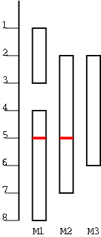
In the figure there are 6 tasks, with start times and finishing times (1,3), (2,5), (2,6), (4,5), (5,8), (5,7). They are scheduled on three machines M1, M2, M3. Clearly 3 machines are needed as can be seen by looking at time 4.

In our greedy algorithm we only go to a new machine when we find a task that cannot be scheduled on the current machines.

1. Why is this called greedy?
2. We are trying to minimize so here greedy means stingy.
3. Like the previous greedy algorithm we are making decisions that are clearly locally optimal, and in this case is globally optimal as well.

Algorithm

Algorithm TaskSchedule(T):
   Input:  A set T of tasks, each with start time si and finishing time fi
           (si≤fi).
   Output: A schedule of the tasks of T on the minimum number of machines.

   m ← 0                                   { current number of machines }
   while T is not empty do
      remove from T a task i with smallest start time
      if there is an Mj having all tasks non-conflicting with i then
         schedule i on Mj
      else
         m ← m+1
         schedule i on Mm

Correctness (i.e. Minimality of m)

Assume the algorithm runs and declares m to be the minimum number of machines needed. We must show that m are really needed.

• Consider the step when the algorithm increases m to its final value and assume the task under consideration is i.
• At this point the current task conflicts with one (or more) task(s) in each of the m-1 machines currently used.
• But all these tasks have start time no later than si since the tasks were processed in order of their start time.
• Since they conflict with i, they each have finishing time after si.
• Hence they all conflict with each other as well (consider time si).
• Hence we really do need m machines.

Complexity

The book asserts that it is easy to see that the algorithm runs in time O(NlogN), but I don't think this is so easy. It is easy to see O(N²).

• The while loop has n iterations.
• You just need to compare the current task with all previous tasks, which shows that the iteration is O(N) and the algorithm is O(N²).
• To get O(log(N)) for each iteration, keep the machines in a heap using as key the latest finishing time assigned to that machine. This tells you when that machine will be free (remember that all tasks assigned so far start no later than si, the current job's start time).
• Check the min element of the tree. If it is free at si, then it is free forever starting at si. We
  1. Remove the machine from the heap (removeMin).
  2. Assign the current job to the removed machine.
  3. Now this machine is free at fi and we re-insert it into the heap.
• If it is not free at si, then no machine is free at si so
  1. Increase m generating a new machine.
  2. Assign i to the new machine m
  3. Insert machine m (which has key fi) into the heap.

Homework: R-5.3

Problem Set 4, Problem 3.
Part A. C-5.3 (Do not argue why your algorithm is correct).
Part B. C-5.4.

Remark: Problem set 4 is now assigned and due 4 Dec 02.