================ Start Lecture #13 ================
Remark: The midterm is coming and will be on chapters 1 and 2. Attend class on monday to vote on the exact day.
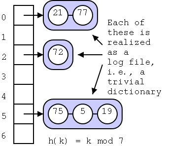
The idea of a hash table is simple: Store the items in an array (as done for log files) but ``somehow'' be able to figure out quickly, i.e., O(1), which array element contains the item (k,e).
We first describe the array, which is easy, and then the ``somehow'', which is not so easy. Indeed in some sense it is impossible. What we can do is produce an implementation that, on the average, performs operations in time O(1).
Allocate an array A of size N of buckets, each able to hold an item. Assume that the keys are integers in the range [0,N-1] and that no two items have the same key. Note that N may be much bigger than n. Now simply store the item (k,e) in A[k].
If everything works as we assumed, we have a very fast implementation: searches, insertions, and removals are O(1). But there are problems, which is why section 2.5 is not finished.
We need a hash function h that maps keys to integers in the range [0,N-1]. Then we will store the item (k,e) in bucket A[h(k)] (we are for now ignoring collisions). This problem is divided into two parts. A hash code assigns to each key a computer integer and then a compression map converts any computer integer into one in the range [0,N-1]. Each of these steps can introduce collisions. So even if the keys were unique to begin with, collisions are an important topic.
A hash code assigns to any key an integer value. The problem we have to solve is that the key may have more bits than are permitted in our integer values. We first view the key as bunch of integer values (to be explained) and then combine these integer values into one.
If our integer values are restricted to 32 bits and our keys are 64
bits, we simply view the high order 32 bits as one value and the low
order as another. In general if
⌈numBitsInKey / numBitsInIntegerValue⌉ = k
we view the key as k integer values. How should we combine the k
values into one?
Simply add the k values.
But, but, but what about overflows?
Ignore them (or use exclusive or instead of addition).
The summing components method gives very many collisions when used for character strings. If 4 characters fill an integer value, then `temphash' and `hashtemp' will give the same value. If one decided to use integer values just large enough to hold one (unicode) character, then there would be many, many common collisions: `t21' and `t12' for one, mite and time for another.
If we call the k integer values x0,...,xk-1, then a better scheme for combining is to choose a positive integer value a and compute Σxiai=x0+x1a+..xn-1an-1.
Same comment about overflows applies.
The authors have found that using a = 33, 37, 39, or 41 worked well for character strings that are English words.
The problem we wish to solve in this section is to map integers in
some, possibly large range, into integers in the range [0,N-1].
This is trivial! Why not map all the integers into 0.
We want to minimize collisions.
This is often called the mod method, especially if you use the ``correct'' definition of mod. One simple way to turn any integer x into one in the range [0,N-1] is to compute |x| mod N. That is we define the hash function h by
h(x) = |x| mod N
(If we used the true mod we would not need the absolute value.)
Choosing N to be prime tends to lower the collision rate, but choosing N to be a power of 2 permits a faster computation since mod with a power of two simply means taking the low order bits.
MAD stands for multiply-add-divide (mod is essentially division). We still use mod N to get the numbers in the range, but we are a little fancier and try to spread the numbers out first. Specifically we define the hash function h via.
h(x) = |ax+b| mod N
The values a and b are chosen (often at random) as positive integers not a multiple of N.
The question we wish to answer is what to do when two distinct keys map to the same value, i.e., when h(k)=h(k'). In this case we have two items to store in one bucket. This discussion also covers the case where we permit multiple items to have the same key.
The idea is simple, each bucket instead of holding an item holds a reference to a container of items. That is each bucket refers to the trivial log file implementation of a dictionary, but only for the keys that map to this container.
The code is simple, you just error check and pass the work off to
the trivial implementation used for the individual bucket.
Algorithm findElement(k):
    B←A[h(k)]
    if B is empty then
        return NO_SUCH_KEY
    // now just do the trivial linear search
    return B.findElement(k)

Algorithm insertItem(k,e):
    if A[h(k)] is empty then
        Create B, an empty sequence-based dictionary
        A[h(k)]←B
    else
        B←A[h(k)]
    B.insertItem(k,e)

Algorithm removeElement(k)
    B←A[h(k)
    if B is empty then
        return NO_SUCH_KEY
    else
        return B.removeElement(k)
Homework: R-2.19
We want the number of keys hashing to a given bucket to be small since the time to find a key at the end of the list is proportional to the size of the list, i.e., to the number of keys that hash to this value.
We can't do much about items that have the same key, so lets consider the (common) case where no two items have the same key.
The average size of a list is n/N, called the load factor, where n is the number of items and N is the number of buckets. Typically, one keeps the load factor below 1.0. The text asserts that 0.75 is common.
What should we do as more items are added to the dictionary? We make an ``extendable dictionary''. That is, as with an extendable array we double N and ``fix everything up'' In the case of an extendable dictionary, the fix up consists of recalculating the hash of every element (since N has doubled). In fact no one calls this an extendable dictionary. Instead one calls this scheme rehashing since one must rehash (i.e., recompute the hash) of each element when N is changed. Also N is normally chosen to be a prime number so instead of doubling, one chooses for the new N the smallest prime number above twice the old N.
Separate chaining involves two data structures: the buckets and the log files. An alternative is to dispense with the log files and always store items in buckets, one item per bucket. Schemes of this kind are referred to as open addressing. The problem they need to solve is where to put an item when the bucket it should go into is already full? There are several different solutions. We study three: Linear probing, quadratic probing, and double hashing.
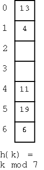
This is the simplest of the schemes. To insert a key k (really I should say ``to insert an item (k,e)'') we compute h(k) and initially assign k to A[h(k)]. If we find that A[h(k)] contains another key, we assign k to A[h(k)+1]. It that bucket is also full, we try A[h(k)+2], etc. Naturally, we do the additions mod N so that after trying A[N-1] we try A[0]. So if we insert (16,e) into the dictionary at the right, we place it into bucket 2.
How about finding a key k (again I should say an item (k,e))?
We first look at A[h(k)]. If this bucket contains the key, we have
found it. If not try A[h(k)+1], etc and of course do it mod N (I will
stop mentioning the mod N). So if
we look for 4 we find it in bucket 1 (after encountering two keys
that hashed to 6).
WRONG!
Or perhaps I should say incomplete. What if the item is not on
the list? How can we tell?
Ans: If we hit an empty bucket then the item is not present (if it
were present we would have stored it in this empty bucket). So 20
is not present.
What if the dictionary is full, i.e., if there are no empty
buckets.
Check to see if you have wrapped all the way around. If so, the
key is not present
What about removals?
Easy, remove the item creating an empty bucket.
WRONG!
Why?
I'm sorry you asked. This is a bit of a mess.
Assume we want to remove the (item with) key 19.
If we simply remove it, and search for 4 we will incorrectly
conclude that it is not there since we will find an empty slot.
OK so we slide all the items down to fill the hole.
WRONG! If we slide 6 into the whole at 5, we
will never be able to find 6.
So we only slide the ones that hash to 4??
WRONG! The rule is you slide all keys that are
not at their hash location until you hit an empty space.
Normally, instead of this complicated procedure for removals, we simple mark the bucket as removed by storing a special value there. When looking for keys we skip over such slots. When an insert hits such a bucket, the insert uses the bucket. (The book calls this a ``deactivated item'' object).
Homework: R-2.20
All the open addressing schemes work roughly the same. The difference is which bucket to try if A[h(k)] is full. One extra disadvantage of linear probing is that it tends to cluster the items into contiguous runs, which slows down the algorithm.
Quadratic probing attempts to spread items out by trying buckets A[h(k)], A[h(k)+1], A[h(k)+4], A[h(k)+9], etc. One problem is that even if N is prime this scheme can fail to find an empty slot even if there are empty slots.
Homework: R-2.21
In double hashing we have two hash functions h and h'. We use h as above and, if A[h(k)] is full, we try A[h(k)+1], A[h(k)+h'(k)], A[h(k)+2h'(k)], etc.
The book says h'(k) is often chosen to be q - (k mod q) for some prime q < N. I note again that if mod were defined correctly this would look more natural, namely (q-k) mod q. We will not consider which secondary hash function h' is good to use.
Homework: R-2.22
A hard choice. Separate chaining seems more space, but that is deceiving since it all depends on the loading factor. In general for each scheme the lower the loading factor, the faster scheme but the more memory it uses.