================ Start Lecture #1 ================
I start at 0 so that when we get to chapter 1, the numbering will agree with the text.
There is a web site for the course. You can find it from my home page, which is http://allan.ultra.nyu.edu/~gottlieb
The course text is Goodrich and Tamassia: ``Algorithm Design: Foundations, Analysis, and Internet Examples.
The major components of the grade will be the midterm, the final, and homeworks. I will post (soon) the weights for each.
We will have a midterm. As the time approaches we will vote in class for the exact date. Please do not schedule any trips during days when the class meets until the midterm date is scheduled.
If you had me for 202, you know that in systems courses I also assign labs. Basic algorithms is not a systems course; there are no labs. There are homeworks and problem sets, very few if any of these will require the computer. There is a distinction between homeworks and problem sets.
Problem sets are
There is a recitation session on tuesdays from 9:30 to 10:45 in room 109. The recitation leader is Sean McLaughlin <seanmcl@cs.nyu.edu>.
Good methods for obtaining help include
I use the upper left board for homework assignments and announcements. I should never erase that board. Viewed as a file it is group readable (the group is those in the room), appendable by just me, and (re-)writable by no one. If you see me start to erase an announcement, let me know.
It is university policy that a student's request for an incomplete be granted only in exceptional circumstances and only if applied for in advance. Naturally, the application must be before the final exam.
We are interested in designing good
algorithms (a step-by-step procedure for performing
some task in a finite amount of time) and good
data structures (a systematic way of organizing and
accessing data).
Unlike v22.102, however, we wish to determine rigorously just how good our algorithms and data structures really are and whether significantly better algorithms are possible.
We will be primarily concerned with the speed (time complexity) of algorithms.
We will emphasize instead and analytic framework that is independent of input and hardware, and does not require an implementation. The disadvantage is that we can only estimate the time required.
Homework: Unless otherwise stated homework problems are from the last section in the current book chapter. R-1.1 and R-1.2.
Designed for human understanding. Suppress unimportant details and describe some parts in natural language (English in this course).
The key difference from reality is the assumption of a very simple memory model: Accessing any memory element takes a constant amount of time. This ignores caching and paging for example. (It also assumes the word-size of a computer is large enough to hold any address. This last assumption is generally valid for modern-day computers, but was not always the case.)
The time required is simply a count of the primitive operations executed. Primitive operations include
Let's start with a simple algorithm (the book does a different simple algorithm, maximum).
Algorithm innerProduct
    Input: Non-negative integer n and two integer arrays A and B of size n.
    Output: The inner product of the two arrays

prod ← 0
for i ← 0 to n-1 do
    prod ← prod + A[i]*B[i]
return prod
The total is thus 1+1+5n+2n+(n+1)+1 = 8n+4.
Let's improve it (a very little bit)
Algorithm innerProductBetter
    Input: Non-negative integer n and two integer arrays A and B of size n.
    Output: The inner product of the two arrays

prod ← A[0]*B[0]
for i ← 1 to n-1 do
    prod ← prod + A[i]*B[i]
return prod
The cost is 4+1+5(n-1)+2(n-1)+n+1 = 8n-1
THIS ALGORITHM IS WRONG!!
If n=0, we access A[0] and B[0], which do not exist. The original
version returns zero as the inner product of empty arrays, which is
arguably correct. The best fix is perhaps to change Non-negative
to Positive
. Let's call this algorithm innerProductBetterFixed.
What about if statements?
Algorithm countPositives
    Input: Non-negative integer n and an integer array A of size n.
    Output: The number of positive elements in A

pos ← 0
for i ← 0 to n-1 do
    if A[i] > 0 then
        pos ← pos + 1
return pos
Let U be the number of updates done.
Consider a recursive version of innerProduct. If the arrays are of size 1, the answer is clearly A[0]B[0]. If n>1, we recursively get the inner product of the first n-1 terms and then add in the last term.
Algorithm innerProductRecursive
    Input: Positive integer n and two integer arrays A and B of size n.
    Output: The inner product of the two arrays

if n=1 then
    return A[0]B[0]
return innerProductRecursive(n-1,A,B) + A[n-1]B[n-1]
How many steps does the algorithm require? Let T(n) be the number of steps required.
Homework: R-1.27
================ Start Lecture #2 ================
Homework: I should have given some last time. It is listed in the notes (search for homework). Also some will be listed this time. BUT, due to the Jewish holiday, none is officially assigned. You can get started if you wish since all will eventually be assigned, but none will be collected next class.
Now we are going to be less precise and worry only about approximate answers for large inputs.
Big-OhNotation
Definition: Let f(n) and g(n) be real-valued functions of a single non-negative integer argument. We write f(n) is O(g(n)) if there is a positive real number c and a positive integer n0 such that f(n)≤cg(n) for all n≥n0.
What does this mean?
For large inputs (n≤n0), f is not much bigger than g (f(n)≤cg(n)).
Examples to do on the board
A few theorems give us rules that make calculating big-Oh easier.
Theorem (arithmetic): Let d(n), e(n), f(n), and g(n) be nonnegative real-valued functions of a nonnegative integer argument and assume d(n) is O(f(n)) and e(n) is O(g(n)). Then
Theorem (transitivity): Let d(n), f(n), and g(n) be nonnegative real-valued functions of a nonnegative integer argument and assume d(n) is O(f(n)) and f(n) is O(g(n)). Then d(n) is O(g(n)).
Theorem (special functions): (Only n varies)
Homework: R-1.19 R-1.20
Definitions: (Common names)
Homework: R-1.10 and R-1.12.
R-1.13: The outer (i) loop is done 2n times. For each outer iteration the inner loop is done i times. Each inner iteration is a constant number of steps so each inner loop is O(i), which is the time for the ith iteration of the outer loop. So the entire outer loop is σO(i) i from 0 to 2n, which is O(n2).
Relativesof the Big-Oh
Recall that f(n) is O(g(n)) if for large n, f is not much bigger than g. That is g is some sort of upper bound on f. How about a definition for the case when g is (in the same sense) a lower bound for f?
Definition: Let f(n) and g(n) be real valued functions of an integer value. Then f(n) is Ω(g(n)) if g(n) is O(f(n)).
Remarks:
Definition: We write f(n) is Θ(g(n)) if both f(n) is O(g(n)) and f(n) is Ω(g(n)).
Remarks We pronounce f(n) is Θ(g(n)) as "f(n) is big-Theta of g(n)"
Examples to do on the board.
Homework: R-1.6
Recall that big-Oh captures the idea that for large n, f(n) is not much bigger than g(n). Now we want to capture the idea that, for large n, f(n) is tiny compared to g(n).
If you remember limits from calculus, what we want is that f(n)/g(n)→0 as n→∞. However, the definition we give does not use limits (it essentially has the definition of a limit built in).
Definition: Let f(n) and g(n) be real valued functions of an integer variable. We say f(n) is o(g(n)) if for any c>0, there is an n0 such that f(n)≤g(n) for all n>n0. This is pronounced as "f(n) is little-oh of g(n)".
Definition: Let f(n) and g(n) be real valued functions of an integer variable. We say f(n) is ω(g(n) if g(n) is o(f(n)). This is pronounced as "f(n) is little-omega of g(n)".
Examples: log(n) is o(n) and x2 is ω(nlog(n)).
Homework: R-1.4. R-1.22
================ Start Lecture #3 ================
Remark: I changed my mind about homework. Too many to have each one really graded. We now have homeworks and problem sets as explained here.
If the asymptotic time complexity is bad, say n5, or horrendous, say 2n, then for large n, the algorithm will definitely be slow. Indeed for exponential algorithms even modest n's (say n=50) are hopeless.
Algorithms that are o(n) (i.e., faster than linear, a.k.a. sub-linear), e.g. logarithmic algorithms, are very fast and quite rare. Note that such algorithms do not even inspect most of the input data once. Binary search has this property. When you look a name in the phone book you do not even glance at a majority of the names present.
Linear algorithms (i.e., Θ(n)) are also fast. Indeed, if the time complexity is O(nlog(n)), we are normally quite happy.
Low degree polynomial (e.g., Θ(n2), Θ(n3), Θ(n4)) are interesting. They are certainly not fast but speeding up a computer system by a factor of 1000 (feasible today with parallelism) means that a Θ(n3) algorithm can solve a problem 10 times larger. Many science/engineering problems are in this range.
It really is true that if algorithm A is o(algorithm B) then for large problems A will take much less time than B.
Definition: If (the number of operations in) algorithm A is o(algorithm B), we call A asymptotically faster than B.
Example:: The following sequence of functions are
ordered by growth rate, i.e., each function is
little-oh of the subsequent function.
log(log(n)), log(n), (log(n))2, n1/3,
n1/2, n, nlog(n), n2/(log(n)), n2,
n3, 2n.
Modest multiplicative constants (as well as immodest additive constants) don't cause too much trouble. But there are algorithms (e.g. the AKS logarithmic sorting algorithm) in which the multiplicative constants are astronomical and hence, despite its wonderful asymptotic complexity, the algorithm is not used in practice.
See table 1.10 on page 20.
Homework: R-1.7
This is hard to type in using html. The book is fine and I will write the formulas on the board.
Definition: The sigma notation: ∑f(i) with i going from a to b.
Theorem: Assume 0<a≠1. Then ∑ai i from 0 to n = (1-an+1)/(1-a).
Proof: Cute trick. Multiply by a and subtract.
Theorem: ∑i from 1 to n = n(n+1)/2.
Proof: Pair the 1 with the n, the 2 with the (n-1), etc. This gives a bunch of (n+1)s. For n even it is clearly n/2 of them. For odd it is the same (look at it).
Recall that logba = c means that bc=a. b is called the base and c is called the exponent.
What is meant by log(n) when we don't specify the base?
I assume you know what ab is. (Actually this is not so obvious. Whatever 2 raised to the square root of 3 means it is not writing 2 down the square root of 3 times and multiplying.) So you also know that ax+y=axay.
Theorem: Let a, b, and c be positive real numbers. To ease writing, I will use base 2 often. This is not needed. Any base would do.
Homework: C-1.12
⌊x⌋ is the greatest integer not greater than x. ⌈x⌉ is the least integer not less than x.
⌊5⌋ = ⌈5⌉ = 5
⌊5.2⌋ = 5 and ⌈5.2⌉ = 6
⌊-5.2⌋ = -6 and ⌈-5.2⌉ = -5
To prove the claim that there is an n greater than 1000, we merely have to note that 1001 is greater than 1001.
To refute the claim that all n are greater than 1000, we merely have to note that 999 is not greater than 1000.
"P implies Q" is the same as "not Q implies not P". So to show that no prime is a square we note that "prime implies not square" is the same is "not (not square) implies not prime", i.e. "square implies not prime", which is obvious.
Assume what you want to prove is false and derive a contradiction.
Theorem: There are an infinite number of primes.
Proof: Assume not. Let the primes be p1 up to pk and consider the number A=p1p2…pk+1. A has remainder 1 when divided by any pi so cannot have any pi as a factor. Factor A into primes. None can be pi (A may or may not be prime). But we assumed that all the primes were pi. Contradiction. Hence our assumption that we could list all the primes was false.
The goal is to show the truth of some statement for all integers n≥1. It is enough to show two things.
Theorem: A complete binary tree of height h has 2h-1 nodes.
Proof:
We write NN(h) to mean the number of nodes in a complete binary tree
of height h.
A complete binary tree of height 1 is just a root so NN(1)=1 and
21-1 = 1.
Now we assume NN(k)=2k-1 nodes for all k<h and consider a complete
binary tree of height h. It is just a complete binary tree of height
h-1 with new leaf nodes added. How many new leaves?
Ans. 2h-1 (this could be proved by induction as a lemma, but
is fairly clear without induction).
Hence NN(h)=NN(h-1)+2h-1 = (2h-1-1)+2h-1 = 2(2h-1)-1=2h-1.
Homework: R-1.9
Very similar to induction. Assume we have a loop with controlling variable i. For example a "for i←0 to n-1" loop. We then associate with the loop a statement S(j) depending on j such that
I favor having array and loop indexes starting at zero. However, here it causes us some grief. We must remember that iteration j occurs when i=j-1.
Example:: Recall the countPositives algorithm
Algorithm countPositives
    Input: Non-negative integer n and an integer array A of size n.
    Output: The number of positive elements in A

pos ← 0
for i ← 0 to n-1 do
    if A[i] > 0 then
        pos ← pos + 1
return pos
Let S(j) be "pos equals the number of positive values in the first j elements of A".
Just before the loop starts S(0) is true vacuously. Indeed that is the purpose of the first statement in the algorithm.
Assume S(j-1) is true before iteration j, then iteration j (i.e., i=j-1) checks A[j-1] which is the jth element and updates pos accordingly. Hence S(j) is true after iteration j finishes.
Hence we conclude that S(n) is true when iteration n concludes, i.e. when the loop terminates. Thus pos is the correct value to return.
================ Start Lecture #4 ================
Skipped for now.
We trivially improved innerProduct (same asymptotic complexity before and after). Now we will see a real improvement. For simplicity I do a slightly simpler algorithm, prefix sums.
Algorithm partialSumsSlow
    Input: Positive integer n and a real array A of size n
    Output: A real array B of size n with B[i]=A[0]+…+A[i]

for i ← 0 to n-1 do
    s ← 0
    for j ← 0 to i do
        s ← s + A[j]
    B[i] ← s
return B
The update of s is performed 1+2+…+n times. Hence the running time is Ω(1+2+…+n)=&Omega(n2). In fact it is easy to see that the time is &Theta(n2).
Algorithm partialSumsFast
    Input: Positive integer n and a real array A of size n
    Output: A real array B of size n with B[i]=A[0]+…+A[i]

s ← 0
for i ← 0 to n-1 do
    s ← s + A[i]
    B[i] ← s
return B
We just have a single loop and each statement inside is O(1), so the algorithm is O(n) (in fact Θ(n)).
Homework: Write partialSumsFastNoTemps, which is also Θ(n) time but avoids the use of s (it still uses i so my name is not great).
Often we have a data structure supporting a number of operations that will be applied many times. For some data structures, the worst-case running time of the operations may not give a good estimate of how long a sequence of operations will take.
If we divide the running time of the sequence by the number of operations performed we get the average time for each operation in the sequence,, which is called the amortized running time.
Why amortized?
Because the cost of the occasional expensive application is
amortized over the numerous cheap application (I think).
Example:: (From the book.) The clearable table. This is essentially an array. The table is initially empty (i.e., has size zero). We want to support three operations.
The obvious implementation is to use a large array A and an integer s indicating the current size of A. More precisely A is (always) of size N (large) and s indicates the extent of A that is currently in use.
We are ignoring a number of error cases.
We start with a size zero table and assume we perform n (legal) operations. Question: What is the worst-case running time for all n operations.
One possibility is that the sequence consists of n-1 add(e) operations followed by one Clear(). The Clear() takes Θ(n), which is the worst-case time for any operation (assuming n operations in total). Since there are n operations and the worst-case is Θ(n) for one of them, we might think that the worst-case sequence would take Θ(n2).
But this is wrong.
It is easy to see that Add(e) and Get(i) are Θ(n).
The total time for all the Clear() operations is O(n) since in total O(n) entries were cleared (since at most n entries were added).
Hence, the amortized time for each operation in the clearable ADT (abstract data type) is O(1), in fact Θ(1).
Overcharge for cheap operations and undercharge expensive so that the excess charged for the cheap (the profit) covers the undercharge (the loss). This is called in accounting an amortization schedule.
Assume the get(i) and add(e) really cost one ``cyber-dollar'', i.e., there is a constant K so that they each take fewer than K primitive operations and we let a ``cyber-dollar'' be K. Similarly, assume that clear() costs P cyber-dollars when the table has P elements in it.
We charge 2 cyber-dollars for every operation. So we have a profit of 1 on each add(e) and we see that the profit is enough to cover next clear() since if we clear P entries, we had P add(e)s.
All operations cost 2 cyber-dollars so n operations cost 2n. Since we have just seen that the real cost is no more than the cyber-dollars spent, the total cost is Θ(n) and the amortized cost is Θ(1).
Very similar to the accounting method. Instead of banking money,
you increase the potential energy. I don't believe we will use this
methods so we are skipping it.
1.5.2 Analyzing an Extendable Array Implementation
We want to let the size of an array grow dynamically (i.e., during execution). The implementation is quite simple. Copy the old array into a new one twice the size. Specifically, on an array overflow instead of signaling an error perform the following steps (assume the array is A and the size is N)
The cost of this growing operation is Θ(N).
Theorem: Given an extendable array A that is initially empty and of size N, the amortized time to perform n add(e) operations is Θ(1).
Proof: Assume one cyber dollar is enough for an add w/o the grow and that N cyber-dollars are enough to grow from N to 2N. Charge 2 cyber dollars for each add; so a profit of 1 for each add w/o growing. When you must do a grow, you had N adds so have N dollars banked.
Book is quite clear. I have little to add.
You might want to know
================ Start Lecture #5 ================
Assume you believe the running time t(n) of an algorithm is Θ(nd) for some specific d and you want to both verify your assumption and find the multiplicative constant.
Make a plot of (n, t(n)/nd). If you are right the points should tend toward a horizontal line and the height of this line is the multiplicative constant.
Homework: R-1.29
What if you believe it is polynomial but don't have a guess for d?
Ans: Use ...
Plot (n, t(n)) on log log paper. If t(n) is Θ(nd), say t(n) approaches bnd, then log(t(n)) approaches log(b)+d(log(n)).
So when you plot (log(n), log(t(n)) (i.e., when you use log log paper), you will see the points approach (for large n) a straight line whose slope is the exponent d and whose y intercept is the multiplicative constant b.
Homework: R-1.30
Stacks implement a LIFO (last in first out) policy. All the action occurs at the top of the stack, primarily with the push(e) and pop operation.
The stack ADT supports
There is a simple implementation using an array A and an integer s (the current size). A[s-1] contains the TOS.
Objection (your honor). The ADT says we can always push. A simple array implementation would need to signal an error if the stack is full.
Sustained! What do you propose instead?
An extendable array.
Good idea.
Homework: Assume a software system has 100 stacks and 100,000 elements that can be on any stack. You do not know how the elements are distributed on the stacks. If you used a normal array based implementation for the stacks, how much memory will you need. What if you use an extendable array based implementation? Now answer the same question, but assume you have θ(S) stacks and Θ(E) elements.
Stacks work great for implementing procedure calls since procedures have stack based semantics. That is, last called is first returned and local variables allocated with a procedure are deallocated when the procedure returns.
So have a stack of "activation records" in which you keep the return address and the local variables.
Support for recursive procedures comes for free. For languages with static memory allocations (e.g., fortran) one can store the local variables with the method. Fortran forbids recursion so that memory allocation can be static. Recursion adds considerably flexibility to a language as some cost in efficiency (not part of this course).
I am review modulo since I believe is no longer taught in high school.
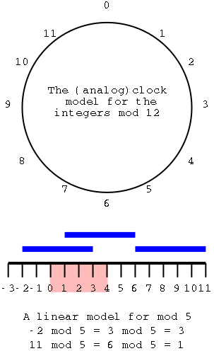
The top diagram shows an almost ordinary analog clock. The major difference is that instead of 12 we have 0. The hands would be useful if this was a video, but I omitted them for the static picture. Positive numbers go clockwise (cw) and negative counter-clockwise (ccw). The numbers shown are the values mod 12. This example is good to show arithmetic. (2-5) mod 12 is obtained by starting at 2 and moving 5 hours ccw, which gives 9. (-7) mod 12 is (0-7) mod 12 is obtained by starting at 0 and going 7 hours ccw, which gives 5.
To get mod 8, divide the circle into 8 hours
instead of 12.
The bottom picture shows mod 5 in a linear fashion. In pink are the 5 values one can get when doing mod 5, namely 0, 1, 2, 3, and 4. I only illustrate numbers from -3 to 11 but that is just due to space limitations. Each blue bar is 5 units long so the numbers at its endpoints are equal mod 5 (since they differ by 5). So you just lay off the blue bar until you wind up in the pink.
Queues implement a FIFO (first in first out) policy. Elements are inserted at the rear and removed from the front using the enqueue and dequeue operations respectively.
The queue ADT supports
My favorite high level language, ada, gets it right in the obvious way: Ada defines both mod and remainder (ada extends the math definition of mod to the case where the second argument is negative).
In the familiar case when x≥0 and y>0 mod and remainder are
equal. Unfortunately the book uses mod sometimes when x<0 and
consequently needs to occasionally add an extra y to get the true mod.
End of personal rant
Returning to relevant issues we note that for queues we need a front and rear "pointers" f and r. Since we are using arrays f and r are actually indexes not pointers. Calling the array Q, Q[f] is the front element of the queue, i.e., the element that would be returned by dequeue(). Similarly, Q[r] is the element into which enqueue(e) would place e. There is one exception: if f=r, the queue is empty so Q[f] is not the front element.
Without writing the code, we see that f will be increased by each dequeue and r will be increased by every enqueue.
Assume Q has n slots Q[0]…Q[N-1] and the queue is initially empty with f=r=0. Now consider enqueue(1); dequeue(); enqueue(2); dequeue(); enqueue(3); dequeue(); …. There is never more than one element in the queue, but f and r keep growing so after N enqueue(e);dequeue() pairs, we cannot issue another operation.
The solution to this problem is to treat the array as circular,
i.e., right after Q[N-1] we find Q[0]. The way to implement this is
to arrange that when either f or r is N-1, adding 1 gives 0 not N.
Similarly for r. So the increment statements become
f←(f+1) mod N
r←(r+1) mod N
Note: Recall that we had some grief due to our starting arrays and loops at 0. For example, the fifth slot of A is A[4] and the fifth iteration of "for i←0 to 30" occurs when i=4. The updates of f and r directly above show one of the advantages of starting at 0; they are less pretty if the array starts at 1.
The size() of the queue seems to be r-f, but this is not always
correct since the array is circular.
For example let N=10 and consider an initially empty queue with f=r=0 that has
enqueue(10)enqueue(20);dequeue();enqueue(30);dequeue();enqueue(40);dequeue()
applied. The queue has one element, f=4, and r=3.
Now apply 6 more enqueue(e) operations
enqueue(50);enqueue(60);enqueue(70);enqueue(80);enqueue(90);enqueue(100)
At this point the array has 7 elements, f=0, and r=3.
Clearly the size() of the queue is not f-r=-3.
It is instead 7, the number of elements in the queue.
The problem is that f in some sense is 10 not 0 since there were 10
enqueue(e) operations. In fact if we kept 2 values for f and 2 for r,
namely the value before the mod and after, then size() would be
fBeforeMod-rBeforeMod. Instead we, use the following inelegant formula.
size() = (r-f+N) mod N
Remark: If java's definition of -3 mod 10 gave 7 (as it
should) instead of -3, we could use the more attractive formula
size() = (r-f) mod N.
Since isEmpty() is simply an abbreviation for the test size()=0, it is just testing if r=f.
Algorithm front():
    if isEmpty() then
        signal an error // throw QueueEmptyException
    return Q[f]
Algorithm dequeue():
    if isEmpty() then
        signal an error // throw QueueEmptyException
    temp←Q[f]
    Q[f]←NULL      // for security or debugging
    f←(f+1) mod N
    return temp
Algorithm enqueue(e):
    if size() = N-1 then
        signal an error // throw QueueFullException
    Q[r]←e
    r←(r+1) mod N
Round Robin processor scheduling is queue based as is fifo disk arm scheduling.
More general processor or disk arm scheduling policies often use priority queues (with various definitions of priority). We will learn how to implement priority queues later this chapter (section 2.4).
Homework: (You may refer to your 202 notes if you wish; mine are on-line based on my home page). How can you interpret Round Robin processor scheduling and fifo disk scheduling as priority queues. That is what is the priority? Same question for SJF (shortest job first) and SSTF (shortest seek time first).
================ Start Lecture #6 ================
Problem Set #1, Problem 1.
The problem set will be officially assigned a little later, but the first
problem in the set is C-2.2
Unlike stacks and queues, the structures in this section support operations in the middle, not just at one or both ends.
The rank of an element in a sequence is the number of elements before it. So if the sequence contains n elements, 0≤rank<n.
A vector storing n elements supports:
Use an array A and store the element with rank r in A[r].
Algorithm insertAtRank(r,e)
   for i = n-1, n-2, ..., r do
      A[i+1]←A[i]
   A[r]←e
   n←n+1

Algorithm removeAtRank(r)
   e←A[r]
   for i = r, r+1, ..., n-2 do
      A[i]←A[i+1]
   n←n-1
   return e
The worst-case time complexity of these two algorithms is Θ(n); the remaining algorithms are all Θ(1).
Homework: When does the worst case occur for insertAtRank(r,e) and removeAtRank(r)?
By using a circular array we can achieve Θ(1) time for insertAtRank(0,e) and removeAtRank(0). Indeed, that is the second problem of the first problem set.
Problem Set #1, Problem 2:
Part 1: C-2.5 from the book
Part 2: This implementation still has worst case complexity
Θ(n). When does the worst case occur?
So far we have been considering what Knuth refers to as sequential allocation, when the next element is stored in the next location. Now we will be considering linked allocation, where each element refers explicitly to the next and/or preceding element(s).
We think of each element as contained in a node, which is a placeholder that also contains references to the preceding and/or following node.
But in fact we don't want to expose Nodes to user's algorithms since this would freeze the possible implementation. Instead we define the idea (i.e., ADT) of a position in a list. The only method available to users is
Given the position ADT, we can now define the methods for the list ADT. The first methods only query a list; the last ones actually modify it.
Now when we are implementing a list we can certainly use the concept of nodes. In a singly linked list each node contains a next link that references the next node. A doubly linked list contains, in addition prev link that references the previous node.
Singly linked lists work well for stacks and queues, but do not perform well for general lists. Hence we use doubly linked lists
Homework: What is the worst case time complexity
of insertBefore for a singly linked list implementation and when does
it occur?
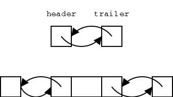
It is convenient to add two special nodes, a header and trailer. The header has just a next component, which links to the first node and the trailer has just a prev component, which links to the last node. For an empty list, the header and trailer link to each other and for a list of size 1, they both link to the only normal node.
In order to proceed from the top (empty) list to the bottom list (with one element), one would need to execute one of the insert methods. Ignoring the abbreviations, this means either insertBefore(p,e) or inserAfter(p,e). But this means that header and/or trailer must be an example of a position, one for which there is no element.
This observation explains the authors' comment above that insertBefore(p,e) cannot be applied if p is the first position. What they mean is that when we permit header and trailer to be positions, then we cannot insertBefore the first position, since that position is the header and the header has no prev. Similarly we cannot insertAfter the final position since that position is the trailer and the trailer has no next. Clearly not the authors' finest hour. Implementation Comment I have not done the implementation. It is probably easiest to have header and trailer have the same three components as a normal node, but have the prev of header and the next of trailer be some special value (say NULL) that can be tested for.
The position p can be header, but cannot be trailer.
Algorithm insertAfter(p,e):
   If p is trailer then signal an error
   Create a new node v
   v.element←e
   v.prev←p
   v.next←p.next
   (p.next).prev←v
   p.next← v
   return v
Do on the board the pointer updates for two cases: Adding a node after an ordinary node and after header. Note that they are the same. Indeed, that is what makes having the header and trailer so convenient.
Homework: Write pseudo code for insertBefore(p,e).
Note that insertAfter(header,e) and insertBefore(trailer,e) appear to be the only way to insert an element into an empty list. In particular, insertFirst(e) fails for an empty list since it performs insertBefore(first()) and first() generates an error for an empty list.
We cannot remove the header or trailer. Notice that removing the only element of a one-element list correctly produces an empty list.
Algorithm remove(p)
   if p is either header or trailer signal an error
   t←p.element
   (p.prev).next←p.next
   (p.next).prev←p.prev
   p.prev←NULL             // for security or debugging
   p.next←NULL
   return t
| Operation | Array | List |
|---|---|---|
| size, isEmpty | O(1) | O(1) |
| atRank, rankOf, elemAtRank | O(1) | O(n) |
| first, last, before, after | O(1) | O(1) |
| replaceElement, swapElements | O(1) | O(1) |
| replaceAtRank | O(1) | O(n) |
| insertAtRank, removeAtRank | O(n) | O(n) |
| insertFirst, insertLast | O(1) | O(1) |
| insertAfter, insertBefore | O(n) | O(1) |
| remove | O(n) | O(1)
|
Define a sequence ADT that includes all the methods of both vector and list ADTs as well as
Sequences can be implemented as either circular arrays, as we did
for vectors) or doubly linked lists, as we did for lists. Neither
clearly dominates the other. Instead it depends on the relative
frequency of the various operations. Circular arrays are faster for
some and doubly liked lists are faster for others as the following
table illustrates.
An ADT for looping through a sequence one element at a time. It has two methods.
When you create the iterator it has all the elements of the sequence. So a typical usage pattern would be
create iterator I for sequence S
while I hasNext
   process nextObject
================ Start Lecture #7 ================
The tree ADT stores elements hierarchically. There is a distinguished root node. All other nodes have a parent of which they are a child. We use nodes and positions interchangeably for trees.
The definition above precludes an empty tree. This is a matter of taste some authors permit empty trees, others do not.
Some more definitions.
We order the children of a binary tree so that the left child comes before the right child.
There are many examples of trees. You learned tree-structured file systems in 202. However, despite what the book says, for Unix/Linux at least the file system does not form a tree (due to hard and symbolic links).
These notes can be thought of as a tree with nodes corresponding to the chapters, sections, subsections, etc.
Games like chess are analyzed in terms of trees. The root is the current position. For each node its children are the positions resulting from the possible moves. Chess playing programs often limit the depth so that the number of examined moves is not too large.
The leaves are constants or variables and the internal nodes are binary arithmetic operations (+,-,*,/). The tree is a proper ordered binary tree (since we are considering binary operators). The value of a leaf is the value of the constant or variable. The value of an internal node is obtained by applying the operator to the values of the children (in order).
Evaluate an arithmetic expression tree on the board.
Homework: R-2.2, but made easier by replacing 21 by 10. If you wish you can do the problem in the book instead (I think it is harder).
We have three accessor methods (i.e., methods that permit us to access the nodes of the tree.
We have four query methods that test status.
Finally generic methods that are useful but not related to the tree structure.
Traversing a tree is a systematic method for accessing or "visiting" each node. We will see and analyze three tree traversal algorithms, inorder, preorder, and postorder. They differ in when we visit an internal node relative to its children. In preorder we visit the node first, in postorder we visit it last, and in inorder, which is only defined for binary trees, we visit the node between visiting the left and right children.
Recursion will be a very big deal in traversing trees!!
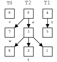
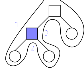
On the right are three trees. The left one just has a root, the right has a root with one leaf as a child, and the middle one has six nodes. For each node, the element in that node is shown inside the box. All three roots are labeled and 2 other nodes are also labeled. That is, we give a name to the position, e.g. the left most root is position v. We write the name of the position under the box. We call the left tree T0 to remind us it has height zero. Similarly the other two are labeled T2 and T1 respectively.
Our goal in this motivation is to calculate the sum the elements in all the nodes of each tree. The answers are, from left to right, 8, 28, and 9.
For a start, lets write an algorithm called treeSum0 that calculates the sum for trees of height zero. In fact the algorithm, will contain two parameters, the tree and a node (position) in that tree, and our algorithm will calculate the sum in the subtree rooted at the given position assuming the position is at height 0. Note this is trivial: since the node has height zero, it has no children and the sum desired is simply the element in this node. So legal invocations would include treeSum0(T0,s) and treeSum0(T2,t). Illegal invocations would include treeSum0(T0,t) and treeSum0(T1,r).
Algorithm treeSum0(T,v)
  Inputs: T a tree; v a height 0 node of T
  Output: The sum of the elements of the subtree routed at v

  Sum←v.element()
  return Sum
Now lets write treeSum1(T,v), which calculates the sum for a node at height 1. It will use treeSum0 to calculate the sum for each child.
Algorithm treeSum1(T,v)
   Inputs: T a tree; v a height 1 node of T
   Output: the sum of the elements of the subtree routed at v

   Sum←v.element()
   for each child c of v
      Sum←Sum+treeSum0(T,c)
   return Sum
OK. How about height 2?
Algorithm treeSum2(T,v)
   Inputs: T a tree; v a height 2 node of T
   Output: the sum of the elements of the subtree routed at v

   Sum←v.element()
   for each child c of v
      Sum←Sum+treeSum1(T,c)
   return Sum
So all we have to do is to write treeSum3, treSum4, ... , where treSum3 invokes treeSum2, treeSum4 invokes treeSum3, ... .
That would be, literally, an infinite amount of work.
Do a diff of treeSum1 and treeSum2.
What do you find are the differences.
In the Algorithm line and in the first comment a 1 becomes a 2.
Why can't we write treeSumI and let I vary?
Because it is illegal to have a varying name for an algorithm.
The solution is to make the I a parameter and write
Algorithm treeSum(i,T,v)
   Inputs: i≥0; T a tree; v a height i node of T
   Output: the sum of the elements of the subtree routed at v

   Sum←v.element()
   for each child c of v
      Sum←Sum+treeSum(i-1,T,c)
   return Sum
This is wrong, why?
Because treeSum(0,T,v) invokes treeSum(-1,c,v), which doesn't
exist because i<0
But treeSum(0,T,v) doesn't have to call anything since v can't have any children (the height of v is 0). So we get
Algorithm treeSum(i,T,v)
   Inputs: i≥0; T a tree; v a height i node of T
   Output: the sum of the elements of the subtree routed at v

   Sum←v.element()
   if i>0 then
      for each child c of v
         Sum←Sum+treeSum(i-1,T,c)
   return Sum
The last two algorithms are recursive; they call themselves. Note that when treeSum(3,T,v) calls treeSum(2,T,c), the new treeSum has new variables Sum and c.
We are pretty happy with our treeSum routine, but ...
The algorithm is wrong! Why?
The children of a height i node need not all be of height i-1.
For example s is hight 2, but its left child w is height 0.
But the only real use we are making of i is to prevent us from recursing when we are at a leaf (the i>0 test). But we can use isInternal instead, giving our final algorithm
Algorithm treeSum(T,v)
   Inputs: T a tree; v a node of T
   Output: the sum of the elements of the subtree routed at v

   Sum←v.element()
   if T.isInternal(v) then
      for each child c of v
         Sum←Sum+treeSum(T,c)
   return Sum
================ Start Lecture #8 ================
Remark:
The department has asked me to make the following announcements.
Our complexity analysis will proceed in a somewhat unusual order. Instead of starting with the bottom (the tree methods in 2.3.1, e.g., is Internal(v)) or the top (the traversals), we will begin by analyzing some middle level procedures assuming the complexities of the low level are as we assert them to be. Then we will analyze the traversals using the middle level routines and finally we will give data structures for trees that achieve our assumed complexity for the low level.
Let's begin!
These will be verified later.
Definitions of depth and height.
Remark: Even our definitions are recursive!
From the recursive definition of depth, the recursive algorithm for its computation essentially writes itself.
Algorithm depth(T,v)
   if T.isRoot(v) then
      return 0
   else
      return 1 + depth(T,T.parent(v))
The complexity is Θ(the answer), i.e. Θ(dv), where dv is the depth of v in the tree T.
Problem Set #1, Problem 3:
Rewrite depth(T,v) without using recursion.
This is quite easy. I include it in the problem set to ensure
that you get practice understanding recursive definitions.
The following algorithm computes the height of a position in a tree.
Algorithm height(T,v):
   if T.isLeaf(v) then
      return 0
   else
      h←0
      for each w in T.children(v) do
         h←max(h,height(T,w))
      return h+1
Remarks on the above algorithm
Theorem: Let T be a tree with n nodes and let cv be the number of children of node v. The sum of cv over all nodes of the tree is n-1.
Proof:
This is trivial! ... once you figure out what it is saying.
The sum gives the total number of children in a tree. But this almost
all nodes. Indeed, there is just one exception.
What is the exception?
The root.
Corollary: Computing the height of an n-node tree has time complexity Θ(n).
Proof:
Look at the code.
The while loop has cv iterations, so by the theorem the
total number of iterations executed is n-1.
Everything else is Θ(1) per iteration.
Do a few on the board. As mentioned above, becoming facile with recursion is vital for tree analyses.
Definition: A traversal is a systematic way of "visiting" every node in a tree.
Visit the root and then recursively traverse each child. More formally we first give the procedure for a preorder traversal starting at any node and then define a preorder traversal of the entire tree as a preorder traversal of the root.
Algorithm preorder(T,v):
   visit node v
   for each child c of v
      preorder(T,c)

Algorithm preorder(T):
   preorder(T,T.root())
Remarks:
Do a few on the board. As mentioned above, becoming facile with recursion is vital for tree analyses.
Theorem: Preorder traversal of a tree with n nodes has complexity Θ(n).
Proof:
Just like height.
The nonrecursive part of each invocation takes O(1+cv)
There are n invocations and the sum of the c's is n-1.
Homework: R-2.3
First recursively traverse each child then visit the root. More formerly
Algorithm postorder(T,v):
   for each child c of v
      postorder(T,c)
   visit node v

Algorithm postorder(T):
   postorder(T,T.root())
Theorem: Preorder traversal of a tree with n nodes has complexity Θ(n).
Proof: The same as for preorder.
================ Start Lecture #9 ================
Note: The following homework should have been assigned last time but wasn't so it is part of homework 9.
Homework: R-2.3
Remarks:
Problem Set 2, Problem 1. Note that the height of a tree is the depth of a deepest node. Extend the height algorithm so that it returns in addition to the height the v.element() for some v that is of maximal depth.
Recall that a binary tree is an ordered tree in which no node has more than two children. The left child is ordered before the right child.
The book adopts the convention that, unless otherwise mentioned, the term "binary tree" will mean "proper binary tree", i.e., all internal nodes have two children. This is a little convenient, but not a big deal. If you instead permitted non-proper binary trees, you would test if a left child existed before traversing it (similarly for right child.)
Will do binary preorder (first visit the node, then the left subtree, then the right subtree, binary postorder (left subtree, right subtree, node) and then inorder (left subtree, node, right subtree).
We have three (accessor) methods in addition to the general tree methods.
Remark: I will not hold you responsible for the proofs of the theorems.
Theorem: Let T be a binary tree having height h and n nodes. Then
Proof:
Base case n=1: Clearly true for all trees having only one node.
Induction hypothesis: Assume true for all trees having at most k nodes.
Main inductive step: prove the assertion for all trees having k+1 nodes. Let T be a tree with k nodes and let h be the height of T.
Remove the root of T. The two subtrees produced each have no
more than k nodes so satisfy the assertion. Since each has height
at most h-1, each has at most 2h-1 leaves. At least
one of the subtrees has height exactly h-1 and hence has at least
h leaves. Put the original tree back together.
One subtree
has at least h leaves, the other has at least 1, so the original
tree has at least h+1. Each subtree has at most 2h-1
leaves and the original root is not a leaf, so the original has at
most 2h leaves.
Theorem:In a binary tree T, the number of leaves is 1 more than the number of internal nodes.
Proof: Again induction on the number of nodes. Clearly true for one node. Assume true for trees with up to n nodes and let T be a tree with n+1 nodes. For example T is the top tree on the right.
Alternate Proof (does not use the pictures):
Corollary: A binary tree has an odd number of nodes.
Proof: #nodes = #leaves + #internal = 2(#internal)+1.
Algorithm binaryPreorder(T,v)
   Visit node v
   if T.isInternal(v) then
      binaryPreorder(T,T.leftChild(v))
      binaryPreorder(T,T.rightChild(v))
Algorithm binaryPretorder(T)
   binaryPreorder(T,T.root())
Algorithm binaryPostorder(T,v)
   if T.isInternal(v) then
      binaryPostorder(T,T.leftChild(v))
      binaryPostorder(T,T.rightChild(v))
   Visit node v
Algorithm binaryPosttorder(T)
   binaryPostorder(T,T.root())
Algorithm binaryInorder(T,v)
   if T.isInternal(v) then
      binaryInorder(T,T.leftChild(v))
   Visit node v
   if T.isInternal(v) then
      binaryInorder(T,T.rightChild(v))
Algorithm binaryIntorder(T)
   binaryPostorder(T,T.root())
================ Start Lecture #10 ================
Remark: Should have mentioned last time the corollary that the number of nodes in a binary tree is odd.
Definition: A binary tree is fully complete if all the leaves are at the same (maximum) depth. This is the same as saying that the sibling of a leaf is a leaf.
Generalizes the above. Visit the node three times, first when ``going left'', then ``going right'', then ``going up''. Perhaps the words should be ``going to go left'', ``going to go right'' and ``going to go up''. These words work for internal nodes. For a leaf you just visit it three times in a row (or you could put in code to only visit a leaf once; I don't do this). It is called an Euler Tour traversal because an Euler tour of a graph is a way of drawing each edge exactly once without taking your pen off the paper. The Euler tour traversal would draw each edge twice but if you add in the parent pointers, each edge is drawn once.
The book uses ``on the left'', ``from below'', ``on the right''. I prefer my names, but you may use either.
Algorithm eulerTour(T,v):
   visit v going left
   if T.isInternal(v) then
      eulerTour(T,T.leftChild(v))
   visit v going right
   if T.isInternal(v) then
      eulerTour(T,T.rightChild(v))
   visit v going up

Algorithm eulerTour(T):
   eulerTour(T,T.root))
Pre- post- and in-order traversals are special cases where two of the three visits are dropped.
It is quite useful to have this three visits. For example here is a nifty algorithm to print and expression tree with parentheses to indicate the order of the operations. We just give the three visits.
Algorithm visitGoingLeft(v):
   if T.isInternal(v) then
      print "("

Algorithm visitGoingRight(v)
   print v.element()

Algorithm visitGoingUp(v)
   if T.isInternal(v) then
      print ")"
Homework: Plug these in to the Euler Tour and show that what you get is the same as
Algorithm printExpression(T,v):
   input: T an expression tree v a node in T.
   if T.isLeaf(v) then
      print v.element()  // for a leaf the element is a value
   else
      print "("
      printExpression(T,T.leftChild(v))
      print v.element()  // for an internal node the element is an operator
      printExpression(T,T.rightChild(v))
      print ")"
Algorithm printExpression(T):
   printExpression(T,T.root())
Problem Set 2 problem 2. We have seen that traversals have complexity Θ(N), where N is the number of nodes in the tree. But we didn't count the costs of the visit()s themselves since the user writes that code. We know that visit() will be called N times, once per node, for post-, pre-, and in-order traversals and will be called 3N times for Euler tour traversal. So if each visit costs Θ(1), the total visit cost will be Θ(N) and thus does not increase the complexity of a traversal. If each visit costs Θ(N), the total visit cost will be Θ(N2) and hence the total traversal cost will be Θ(N2). The same analysis works for any visit cost providing all the visits cost the same. For this problem we will be considering a variable cost visits. In particular, assume that the cost of visiting a node v is the height of v (so roots can be expensive to visit, but leaves are free).
Part A. How many nodes N are in a fully complete binary tree of height h?
Part B. How many nodes are at height i in a fully complete binary tree of height h? What is the total cost of visiting all the nodes at height i?
Part C. Write a formula using Σ (sum) for the total cost of visiting all the nodes. This is very easy given B.
One point extra credit. Show that the sum you wrote in part C is Θ(N).
Part D. Continue to assume the cost of visiting a node equals its height. Describe a class of binary trees for which the total cost of visiting the nodes is θ(N2). Naturally these will not be fully complete binary trees. Hint do problem 3.
We store each node as the element of a vector. Store the root in element 1 of the vector and the key idea is that we store the two children of the element at rank r in the elements at rank 2r and 2r+1.
Draw a fully complete binary tree of height 3 and show where each element is stored.
Draw an incomplete binary tree of height 3 and show where each element is stored and that there are gaps.
There must be a way to tell leaves from internal nodes. The book
doesn't make this explicit. Here is an explicit example.
Let the vector S be given. With a vector we have the current size.
S[0] is not used. S[1] has a pointer to the root node (or contains
the root node if you prefer. For each S[i], S[i] is null (a special
value) if the corresponding node doesn't exist). Then to see if the
node v at rank i is a leaf, look at 2i. If 2i exceeds S.size() then v
is a leaf since it has no children. Similarly if S[2i] is null, v is
a leaf. Otherwise v is external.
How do you know that if S[2i] is null, then s[2i+1] will be null?
Ans: Our binary trees are proper.
This implementation is very fast. Indeed all tree operations are O(1) except for positions() and elements(), which produce n results and take time Θ(n).
Homework: R-2.7
However, this implementation can waste a lot of space since many of the entries in S might be unused. That is there may be many i for which S[i] is null.
Problem Set 2 problem 3. Give a tree with fewer than 20 nodes for which S.size() exceeds 100. Give a tree with fewer than 25 nodes for which S.size() exceeds 1000. Give a tree with fewer than 100 nodes for which S.size() exceeds a million.
Represent each node by a quadruple.
Once again the algorithms are all O(1) except for positions() and elements(), which are Θ(n).
The space is Θ(n) which is much better that for the vector implementation. The constant is larger however since three pointers are stored for each position rather than one index.
The only difference is that we don't know how many children each node has. We could store k child pointers and say that we cannot process a tree having more than k children with the same parent.
Clearly we don't like this limit. Moreover, if we choose k moderate, say k=10. We are limited to 10-ary trees and for 3-ary trees most of the space is wasted.
So instead of storing the child references in the node, we store just one reference to a container. The container has references to the children. Imaging implementing the container as an extendable array.
Since a node v contains an arbitrary number of children, say Cv, the complexity of the children(v) iterator is Θ(Cv).
================ Start Lecture #11 ================
Up to now we have not considered elements that must be retrieved in a fixed order. But often in practice we assign a priority to each item and want the most important (highest priority) item first. (For some reason that I don't know, low numbers are often used to represent high priority.)
For example consider processor scheduling from Operating Systems (202). The simplest scheduling policy is FCFS for which a queue of ready processors is appropriate. But if we want SJF (short job first) then we want to extract the ready process that has the smallest remaining time. Hence a FIFO queue is not appropriate.
For a non-computer example,consider managing your todo list. When you get another item to add, you decide on its importance (priority) and then insert the item into the todo list. When it comes time to perform an item, you want to remove the highest priority item. Again the behavior is not FIFO.
To return items in order, we must know when one item is less than another. For real numbers this is of course obvious.
We assume that each item has a key on which the priority is to be based. For the SJF example given above, the key is the time remaining. For the todo example, the key is the importance.
We assume the existence of an order relation (often called a total order) written ≤ satisfying for all keys s, t, and u.
Remark: For the complex numbers no such ordering exists that extends the natural ordering on the reals and imaginaries. This is unofficial (not part of 310).
Is it OK to define s≤t for all s and t?
No. That would not be antisymmetric.
Definition: A priority queue is a container of elements each of which has an associated key supporting the following methods.
Users may choose different comparison functions for the same data. For example, if the keys are longitude,latitude pairs, one user may be interested in comparing longitudes and another latitudes. So we consider a general comparator containing methods.
Given a priority queue it is trivial to sort a collection of elements. Just insert them and then do removeMin to get them in order. Written formally this is
Algorithm PQ-Sort(C,P)
   Input: an n element sequence C and an empty priority queue P
   Output: C with the elements sorted

   while not C.isEmpty() do
      e←C.removeFirst()
      P.insertItem(e,e)  // We are sorting on the element itself.

   while not P.isEmpty()
      C.insertLast(P.removeMin())
So whenever we give an implementation of a priority queue, we are also giving a sorting algorithm. Two obvious implementations of a priority queue give well known (but slow) sorts. A non-obvious implementation gives a fast sort. We begin with the obvious.
So insertItem() takes Θ(1) time and hence takes Θ(N) to insert all n items of C. But remove min, requires we go through the entire list. This requires time Θ(k) when there are k items in the list. Hence to remove all the items requires Θ(n+(n-1)+...+1) = Θ(N2) time.
This sorting algorithm is normally called selection sort since the dominant step is selecting the minimum each time.
Now removeMin() is trivial since it is just removeFirst(). But insertItem is Θ(k) when there are k items already in the priority queue since you must step through to find the correct location to insert and then slide the remaining elements over.
This sorting element is normally called insertion sort since the dominant effort is inserting each element.
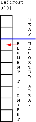
We now consider the non-obvious implementation of a priority queue that gives a fast sort (and a fast priority queue). Since the priority queue algorithm will perform steps with complexity Θ(height of tree), we want to keep the height small. The way to do this is to fully use each level.
Definition: A binary tree of height h is complete if the levels 0,...,h-1 contain the maximum number of elements and on level h-1 all the internal nodes are to the left of all the leaves.
Remarks:
Definition: A tree storing a key at each node satisfies the heap-order property if, for every node v other than the root, the key at v is no smaller than the key at v's parent.
Definition: A heap is a complete binary tree satisfying the heap order property.
Definition: The last node of a heap is the right most internal node in level h-1.
Remark: As written the ``last node'' is really the last internal node. However, we actually don't use the leaves to store keys so in some sense ``last node'' is the last (significant) node.
With a heap it is clear where the minimum is located, namely at the root. We will also use last a reference to the last node since insertions will occur at the first node after last.
Theorem: A heap with storing n keys has height ⌈log(n+1)⌉
Proof:
Corollary: If we can implement insert and removeMin in time Θ(height), we will have implemented the priority queue operations in logarithmic time (our goal).
Since we know that a heap is complete is efficient to use the vector representation of a binary tree. We can actually not bother with the leaves since we don't ever use them. We call the last node w (remember that is the last internal node). Its index in the vector representation is n, the number of keys in the heap. We call the first leaf z; its index is n+1. Node z is where we will insert a new element and is called the insertion position.
================ Start Lecture #12 ================
Remarks (sent to mailing list on thurs):
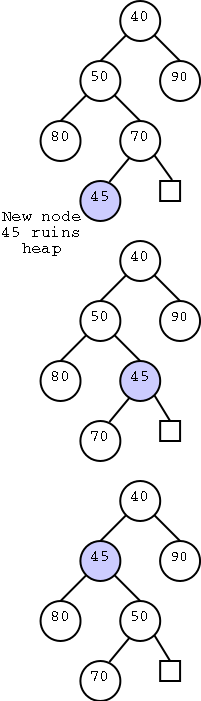
This looks trivial. Since we know n, we can find n+1 and hence the reference to node z in O(1) time. But there is a problem; the result might not be a heap since the new key inserted at z might be less than the key stored at u the parent of z. Reminiscent of bubble sort, we need to bubble the value in z up to the correct location.
We compare key(z) with key(u) and swap the items if necessary. In the diagram on the right we added 45 and then had to swap it with 70. But now 45 is still less than its parent so we need to swap again. At worst we need to go all the way up to the root. But that is only Θ(n) as desired. Let's slow down and see that this really works.
Great. It works (i.e., is a heap) and there can only be O(log(n)) swaps because that is the height of the tree.
But wait! What I showed is that it only takes O(n) steps. Is each step O(1)?
Comparing is clearly O(1) and swapping two fixed elements is also O(1). Finding the parent of a node is easy (integer divide the vector index by 2). Finally, it is trivial to find the new index for the insertion point (just increase the insertion point by 1).
Remark: It is not as trivial to find the new insertion point using a linked implementation.
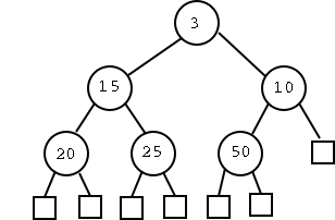
Homework: Show the steps for inserting an element
with key 2 in the heap of Figure 2.41.
Trivial, right? Just remove the root since that must contain an
element with minimum key. Also decrease n by one.
Wrong!
What remains is TWO trees.
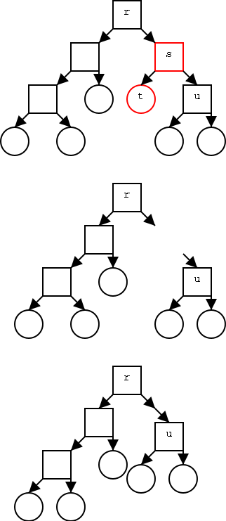
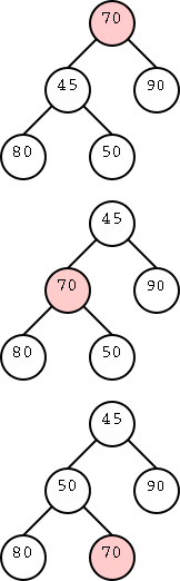
We do want the element stored at the root but we must put some other element in the root. The one we choose is our friend the last node.
But the last node is likely not to be a valid root, i.e. it will destroy the heap property since it will likely be bigger than one of its new children. So we have to bubble this one down. It is shown in pale red on the right and the procedure explained below. We also need to find a new last node, but that really is trivial: It is the node stored at the new value of n.
If the new root is the only internal node then we are done.
If only one child of the root is internal (it must be the left child) compare its key with the key of the root and swap if needed.
If both children of the root are internal, choose the child with the smaller key and swap with the root if needed.
The original last node, became the root, and now has been bubbled down to level 1. But it might still be bigger than a child so we keep bubbling. At worst we need Θ(h) bubbling steps, which is again logarithmic in n as desired.
Homework: R-2.16
| Operation | Time |
|---|---|
| size, isEmpty | O(1) |
| minElement, minKey | O(1) |
| insertItem | Θ(log n) |
| removeMin | Θ(log n) |
The table on the right gives the performance of the heap implementation of a priority queue. As desired, the main operations have logarithmic time complexity. It is for this reason that heap sort is fast.
The goal is to sort a sequence S. We return to the PQ-sort where we insert the elements of S into a priority queue and then use removeMin to obtain the sorted version. When we use a heap to implement the priority queue, each insertion and removal takes O(log(n)) so the entire algorithm takes O(nlog(n)). The heap implementation of PQ-sort is called heap-sort and we have shown
Theorem: The heap-sort algorithm sorts a sequence of n comparable elements in O(nlog(n)) time.
 In place means that we use the space occupied by the input.
More precisely, it means that the space required is just the input +
O(1) additional memory. The algorithm above required Θ(n)
addition space to store the heap.
In place means that we use the space occupied by the input.
More precisely, it means that the space required is just the input +
O(1) additional memory. The algorithm above required Θ(n)
addition space to store the heap.
The in place heap-sort of S assumes that S is implemented as an array and proceeds as follows (This presentation, beyond the definition of ``in place'' is unofficial; i.e., it will not appear on problem sets or exams)
If you are given at the beginning all n elements that are to be inserted, the total insertion time for all inserts can be reduced to O(n) from O(nlog(n)). The basic idea assuming n=2n-1 is
Sometimes we wish to extend the priority queue ADT to include a locater that always points to the same element even when the element moves around. So if x is in a priority queue and another item is inserted, x may move during the up-heap bubbling, but the locater of x continues to refer to x.
Method | Unsorted Sequence | Sorted Sequence | Heap |
|---|---|---|---|
| size, isEmpty | O(1) | O(1) | O(1) |
| minElement, minKey | O(n) | O(1) | O(1) |
| insertItem | O(1) | O(n) | O(log(n)) |
| removeMin | O(n) | O(1) | O(log(n)) |
Dictionaries, as the name implies are used to contain data that may later be retrieved. Associated with each element is the key used for retrieval.
For example consider an element to be one student's NYU transcript and the key would be the student id number. So given the key (id number) the dictionary would return the entire element (the transcript).
A dictionary stores items, which are key-element (k,e) pairs.
We will study ordered dictionaries in the next chapter when we consider searching. Here we consider unordered dictionaries. So, for example, we do not support findSmallestKey. the methods we do support are
Just store the items in a sequence.
================ Start Lecture #13 ================
Remark: The midterm is coming and will be on chapters 1 and 2. Attend class on monday to vote on the exact day.
The idea of a hash table is simple: Store the items in an array (as done for log files) but ``somehow'' be able to figure out quickly, i.e., O(1), which array element contains the item (k,e).
We first describe the array, which is easy, and then the ``somehow'', which is not so easy. Indeed in some sense it is impossible. What we can do is produce an implementation that, on the average, performs operations in time O(1).
Allocate an array A of size N of buckets, each able to hold an item. Assume that the keys are integers in the range [0,N-1] and that no two items have the same key. Note that N may be much bigger than n. Now simply store the item (k,e) in A[k].
If everything works as we assumed, we have a very fast implementation: searches, insertions, and removals are O(1). But there are problems, which is why section 2.5 is not finished.
We need a hash function h that maps keys to integers in the range [0,N-1]. Then we will store the item (k,e) in bucket A[h(k)] (we are for now ignoring collisions). This problem is divided into two parts. A hash code assigns to each key a computer integer and then a compression map converts any computer integer into one in the range [0,N-1]. Each of these steps can introduce collisions. So even if the keys were unique to begin with, collisions are an important topic.
A hash code assigns to any key an integer value. The problem we have to solve is that the key may have more bits than are permitted in our integer values. We first view the key as bunch of integer values (to be explained) and then combine these integer values into one.
If our integer values are restricted to 32 bits and our keys are 64
bits, we simply view the high order 32 bits as one value and the low
order as another. In general if
⌈numBitsInKey / numBitsInIntegerValue⌉ = k
we view the key as k integer values. How should we combine the k
values into one?
Simply add the k values.
But, but, but what about overflows?
Ignore them (or use exclusive or instead of addition).
The summing components method gives very many collisions when used for character strings. If 4 characters fill an integer value, then `temphash' and `hashtemp' will give the same value. If one decided to use integer values just large enough to hold one (unicode) character, then there would be many, many common collisions: `t21' and `t12' for one, mite and time for another.
If we call the k integer values x0,...,xk-1, then a better scheme for combining is to choose a positive integer value a and compute Σxiai=x0+x1a+..xn-1an-1.
Same comment about overflows applies.
The authors have found that using a = 33, 37, 39, or 41 worked well for character strings that are English words.
The problem we wish to solve in this section is to map integers in
some, possibly large range, into integers in the range [0,N-1].
This is trivial! Why not map all the integers into 0.
We want to minimize collisions.
This is often called the mod method, especially if you use the ``correct'' definition of mod. One simple way to turn any integer x into one in the range [0,N-1] is to compute |x| mod N. That is we define the hash function h by
h(x) = |x| mod N
(If we used the true mod we would not need the absolute value.)
Choosing N to be prime tends to lower the collision rate, but choosing N to be a power of 2 permits a faster computation since mod with a power of two simply means taking the low order bits.
MAD stands for multiply-add-divide (mod is essentially division). We still use mod N to get the numbers in the range, but we are a little fancier and try to spread the numbers out first. Specifically we define the hash function h via.
h(x) = |ax+b| mod N
The values a and b are chosen (often at random) as positive integers not a multiple of N.
The question we wish to answer is what to do when two distinct keys map to the same value, i.e., when h(k)=h(k'). In this case we have two items to store in one bucket. This discussion also covers the case where we permit multiple items to have the same key.
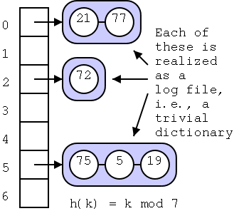
The idea is simple, each bucket instead of holding an item holds a reference to a container of items. That is each bucket refers to the trivial log file implementation of a dictionary, but only for the keys that map to this container.
The code is simple, you just error check and pass the work off to
the trivial implementation used for the individual bucket.
Algorithm findElement(k):
    B←A[h(k)]
    if B is empty then
        return NO_SUCH_KEY
    // now just do the trivial linear search
    return B.findElement(k)

Algorithm insertItem(k,e):
    if A[h(k)] is empty then
        Create B, an empty sequence-based dictionary
        A[h(k)]←B
    else
        B←A[h(k)]
    B.insertItem(k,e)

Algorithm removeElement(k)
    B←A[h(k)
    if B is empty then
        return NO_SUCH_KEY
    else
        return B.removeElement(k)
Homework: R-2.19
We want the number of keys hashing to a given bucket to be small since the time to find a key at the end of the list is proportional to the size of the list, i.e., to the number of keys that hash to this value.
We can't do much about items that have the same key, so lets consider the (common) case where no two items have the same key.
The average size of a list is n/N, called the load factor, where n is the number of items and N is the number of buckets. Typically, one keeps the load factor below 1.0. The text asserts that 0.75 is common.
What should we do as more items are added to the dictionary? We make an ``extendable dictionary''. That is, as with an extendable array we double N and ``fix everything up'' In the case of an extendable dictionary, the fix up consists of recalculating the hash of every element (since N has doubled). In fact no one calls this an extendable dictionary. Instead one calls this scheme rehashing since one must rehash (i.e., recompute the hash) of each element when N is changed. Also N is normally chosen to be a prime number so instead of doubling, one chooses for the new N the smallest prime number above twice the old N.
Separate chaining involves two data structures: the buckets and the log files. An alternative is to dispense with the log files and always store items in buckets, one item per bucket. Schemes of this kind are referred to as open addressing. The problem they need to solve is where to put an item when the bucket it should go into is already full? There are several different solutions. We study three: Linear probing, quadratic probing, and double hashing.
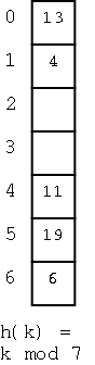
This is the simplest of the schemes. To insert a key k (really I should say ``to insert an item (k,e)'') we compute h(k) and initially assign k to A[h(k)]. If we find that A[h(k)] contains another key, we assign k to A[h(k)+1]. It that bucket is also full, we try A[h(k)+2], etc. Naturally, we do the additions mod N so that after trying A[N-1] we try A[0]. So if we insert (16,e) into the dictionary at the right, we place it into bucket 2.
How about finding a key k (again I should say an item (k,e))?
We first look at A[h(k)]. If this bucket contains the key, we have
found it. If not try A[h(k)+1], etc and of course do it mod N (I will
stop mentioning the mod N). So if
we look for 4 we find it in bucket 1 (after encountering two keys
that hashed to 6).
WRONG!
Or perhaps I should say incomplete. What if the item is not on
the list? How can we tell?
Ans: If we hit an empty bucket then the item is not present (if it
were present we would have stored it in this empty bucket). So 20
is not present.
What if the dictionary is full, i.e., if there are no empty
buckets.
Check to see if you have wrapped all the way around. If so, the
key is not present
What about removals?
Easy, remove the item creating an empty bucket.
WRONG!
Why?
I'm sorry you asked. This is a bit of a mess.
Assume we want to remove the (item with) key 19.
If we simply remove it, and search for 4 we will incorrectly
conclude that it is not there since we will find an empty slot.
OK so we slide all the items down to fill the hole.
WRONG! If we slide 6 into the whole at 5, we
will never be able to find 6.
So we only slide the ones that hash to 4??
WRONG! The rule is you slide all keys that are
not at their hash location until you hit an empty space.
Normally, instead of this complicated procedure for removals, we simple mark the bucket as removed by storing a special value there. When looking for keys we skip over such slots. When an insert hits such a bucket, the insert uses the bucket. (The book calls this a ``deactivated item'' object).
Homework: R-2.20
All the open addressing schemes work roughly the same. The difference is which bucket to try if A[h(k)] is full. One extra disadvantage of linear probing is that it tends to cluster the items into contiguous runs, which slows down the algorithm.
Quadratic probing attempts to spread items out by trying buckets A[h(k)], A[h(k)+1], A[h(k)+4], A[h(k)+9], etc. One problem is that even if N is prime this scheme can fail to find an empty slot even if there are empty slots.
Homework: R-2.21
In double hashing we have two hash functions h and h'. We use h as above and, if A[h(k)] is full, we try A[h(k)+1], A[h(k)+h'(k)], A[h(k)+2h'(k)], etc.
The book says h'(k) is often chosen to be q - (k mod q) for some prime q < N. I note again that if mod were defined correctly this would look more natural, namely (q-k) mod q. We will not consider which secondary hash function h' is good to use.
Homework: R-2.22
A hard choice. Separate chaining seems more space, but that is deceiving since it all depends on the loading factor. In general for each scheme the lower the loading factor, the faster scheme but the more memory it uses.
================ Start Lecture #14 ================
Remark: From robin simon
The last day for students to withdraw is Nov. 5th.
Therefore the exam should be returned at least a week
before then.
We just studied unordered dictionaries at the end of chapter 2. Now we want to extend the study to permit us to find the "next" and "previous" items. More precisely we wish to support, in addition to findElement(k), insertItem(k,e), and removeElement(k), the new methods
We naturally signal an exception if no such item exists. For example if the only keys present are 55, 22, 77, and 88, then closestKeyAfter(90) or closestElemBefore(2) each signal an exception.
We begin with the most natural implementation.
We use the sorted vector implementation from chapter 2 (we used it as a simple implementation of a priority queue). Recall that this keeps the items sorted in key order. Hence it is O(n) for inserts and removals, which is slow; however, we shall see that it is fast for finding and element and for the four new methods closestKeyBefore(k) and friends. We call this a lookup table.
The space required is Θ(n) since we grow and shrink the array supporting the vector (see extendable arrays).
As indicated the key favorable property of a lookup table is that it is fast for (surprise) lookups using the binary search algorithm that we study next.
In this algorithm we are searching for the rank of the item containing a key equal to k. We are to return a special value if no such key is found.
The algorithm maintains two variables lo and hi, which are respectively lower and upper bounds on the rank where k will be found (assuming it is present).
Initially, the key could be anywhere in the vector so we start with lo=0 and hi=n-1. We write key(r) for the key at rank r and elem(r) for the element at rank r.
We then find mid, the rank (approximately) halfway between lo and hi and see how the key there compares with our desired key.
Some care is need in writing the algorithm precisely as it is easy to have an ``off by one error''. Also we must handle the case in which the desired key is not present in the vector. This occurs when the search range has been reduced to the empty set (i.e., when lo exceeds hi).
Algorithm BinarySearch(S,k,lo,hi):
    Input:  An ordered vector S containing (key(r),elem(r)) at rank r
            A search key k
            Integers lo and hi
    Output: An element of S with key k and rank between lo and hi.
            NO_SUCH_KEY if no such element exits

If lo > hi then
    return NO_SUCH_KEY                    // Not present

mid ← ⌊(lo+hi)/2⌋
if k = key(mid) then
    return elem(mid)                     // Found it
if k < key(mid) then
    return BinarySearch(S,k,lo,mid-1)    // Try bottom ``half''
if k > key(mid) then
    return BinarySearch(S,k,mid+1,hi)    // Try top ``half''
Do some examples on the board.
It is easy to see that the algorithm does just a few operations per recursive call. So the complexity of Binary Search is Θ(NumberOfRecursions). So the question is "How many recursions are possible for a lookup table with n items?".
The number of eligible ranks (i.e., the size of the range we still must consider) is hi-lo+1.
The key insight is that when we recurse, we have reduced the range to at most half of what it was before. There are two possibilities, we either tried the bottom or top ``half''. Let's evaluate hi-lo+1 for the bottom and top half. Note that the only two possibilities for ⌊(lo+hi)/2⌋ are (lo+hi)/2 or (lo+hi)/2-(1/2)=(lo+hi-1)/2
Bottom:
(mid-1)-lo+1 = mid-lo = ⌊(lo+hi)/2⌋-lo
≤ (lo+hi)/2-lo = (hi-lo)/2<(hi-lo+1)/2
Top:
hi-(mid+1)+1 = hi-mid = hi-⌊(lo+hi)/2⌋
≤ hi-(lo+hi-1)/2 = (hi-lo+1)/2
So the range starts at n and is halved each time and remains an integer (i.e., if a recursive call has a range of size x, the next recursion will be at most ⌊x/2⌋).
================ Start Lecture #15 ================
Write on the board 10 times
(X-1)/2 ≤ ⌊X/2⌋ &le X/2
If B ≤ A, then Z-A ≤ Z-B
How many recursions are possible? If the range is ever zero, we stop (and declare the key is not present) so the longest we can have is the number of times you can divide by 2 and stay at least 1. That number is Θ(log(n)) showing that binary search is a logarithmic algorithm.
Problem Set 3, Problem 1 Write the algorithm closestKeyBefore. It uses the same idea as BinarySearch.
When you do question 1 you will see that the complexity is Θ(log(n)). Proving this is not hard but is not part of the problem set.
When you do question 1 you will see that closestElemBefore, closestKeyAfter, and closestElemAfter are all very similar to closestKeyBefore. Hence they are all logarithmic algorithms. Proving this is not hard but is not part of the problem set.
| Method | Log File | Lookup Table |
|---|---|---|
| findElement | O(n) | O(log n) |
| insertItem | O(1) | O(n) |
| removeElement | O(n) | O(n) |
| closestKeyBefore | O(n) | O(log n) |
| closestElemBefore | O(n) | O(log n) |
| closestKeyAfter | O(n) | O(log n) |
| closestElemAfter | O(n) | O(log n) |
Our goal now is to find a better implementation so that all the complexities are logarithmic. This will require us to shift from vectors to trees.
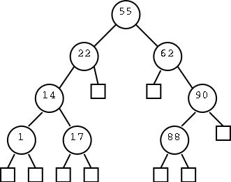
This section gives a simple tree-based implementation, which alas fails to achieve the logarithmic bounds we seek. But it is a good start and motivates the AVL trees we study in 3.2 that do achieve the desired bounds.
Definition: A binary search tree is a tree in which each internal node v stores an item such that the keys stored in every node in the left subtree of v are less than or equal to the key at v which is less than or equal to every key stored in the right subtree.
From the definition we see easily that an inorder traversal of the tree visits the internal nodes in nondecreasing order of the keys they store.
You search by starting at the root and going left or right if the desired key is smaller or larger respectively than the key at the current node. If the key at the current node is the key you seek, you are done. If you reach a leaf the desired key is not present.
Do some examples using the tree on the right. E.g. search for 17, 80, 55, and 65.
Homework: R-3.1 and R-3.2
Here is the formal algorithm described above.
Algorithm TreeSearch(k,v)
Input:  A search key k and a node v of a binary search tree.
Output: A node w in the subtree routed at v such that either
        w is internal and k is stored at w or
        w is a leaf where k would be stored if it existed

if v is a leaf then
    return v
if k=k(v) then
    return v
if k<k(v) then
    return TreeSearch(k,T.leftChild(v))
if k>k(v) then
    return TreeSearch(k,T.rightChild(v))
Draw a tree on the board and illustrate both finding a k and no such key exists.
It is easy to see that only a couple of operations are done per recursive call and that each call goes down a level in the tree. Hence the complexity is O(height).
So the question becomes "How high is a tree with n nodes?". As we saw last chapter the answer is "It depends.".
Next section we will learn a technique for keeping trees low.
To insert an item with key k, first execute w←TreeSearch(k,T.root()). Recall that if w is internal, k is already in w, and if w is a leaf, k "belongs" in w. So we proceed as follows.
Draw examples on the board showing both cases (leaf and internal returned).
Once again we perform a constant amount of work per level of the tree implying that the complexity is O(height).
This is the trickiest part, especially in one case as we describe below. The key concern is that we cannot simply remove an item from an internal node and leave a hole as this would make future searches fail. The beginning of the removal technique is familiar: w=TreeSearch(k,T.root()). If w is a leaf, k is not present, which we signal.
If w is internal, we have found k, but now the fun begins.
Returning the element with key k is easy, it is the element
stored in w.
We need to actually remove w, but we cannot leave a hole.
There are three cases.
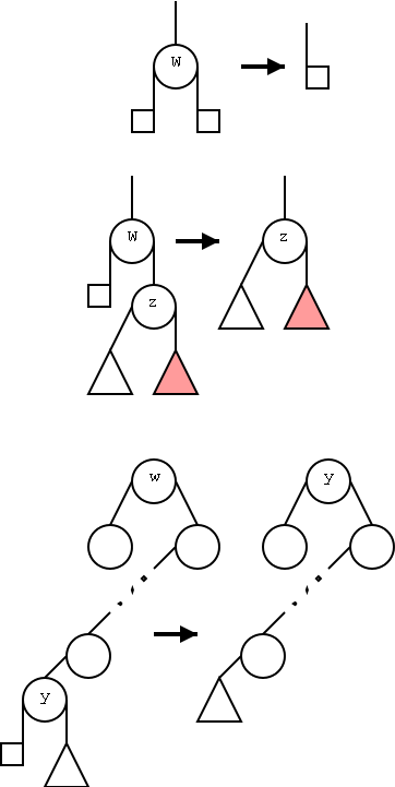
| Method | Time |
|---|---|
| size, isEmpty | O(1) |
| findElement, insertItem, removeElement | O(h) |
| findAllElements, removeAllElements | O(h+s) |
We have seen that findElement, insertItem, and removeElement have complexity O(height). It is also true, but we will not show it, that one can implement findAllElements and removeAllElements in time O(height+numberOfElements). You might think removeAllElements should be constant time since the resulting tree is just a root so we can make it in constant time. But removeAllElements must also return an iterator that when invoked must generate each of the elements removed.
In a sense that we will not make precise, binary search trees have logarithmic performance since `most' trees have logarithmic height.
Nonetheless we know that there are trees with height Θ(n). You produced several of them for problem set 2. For these trees binary search takes linear time, i.e., is slow. Our goal now is to fancy up the implementation so that the trees are never very high. We can do this since the trees are not handed to us. Instead they are build up using our insertItem method.
================ Start Lecture #16 ================
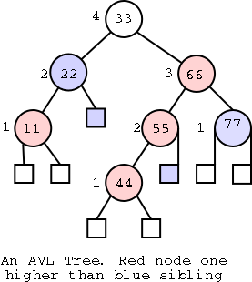
Named after its inventors Adel'son-Vel'skii and Landis.
Definition: An AVL tree is a binary search tree that satisfies the height-balance property, which means that for every internal node, the height of the two children can differ by at most 1.
Homework: R-3.3
Since the algorithms for an AVL tree require the height to be computed and this is an expensive operation, each node of an AVL tree contains its height (say as v.height()).
Remark: You can actually be fancier and store just two bits to tell whether the node has the same height as its sibling, one greater, or one smaller.
We see that the height-balance property prevents the tall skinny trees you developed in problem set 2. But is it really true that the height must be O(log(n))?
Yes it is and we shall now prove it. Actually we will prove instead that an AVL tree of height h has at least 2(h/2)-1 internal nodes from which the desired result follows easily.
Lemma: An AVL tree of height h has at least 2(h/2)-1 internal nodes.
Proof: Let n(h) be the minimum number of internal nodes in an AVL tree of height h.
n(1)=1 and n(2)=2. So the lemma holds for h=1 and h=2.
Here comes the key point.
Consider an AVL tree of height h≥3
and the minimum number of nodes. This tree is composed of a root,
and two subtrees. Since the whole tree has the minimum number of
nodes for its height so do the subtrees. For the big tree to be of
height h, one of the subtrees must be of height h-1. To get the
minimum number of nodes the other subtree is of height h-2.
Why can't the other subtree be of height h-3 or h-4?
The height of siblings can differ by at most 1!
What the last paragraph says in symbols is that for h≥3,
n(h) = 1+n(h-1)+n(h-2)
The rest is just algebra, i.e. has nothing to do with trees, heights, searches, siblings, etc.
n(h) > n(h-1) so n(h-1) > n(h-2). Hence
n(h) > n(h-1)+n(h-2) > 2n(h-2)
Really we could stop here. We have shown that n(h) at least doubles when h goes up by 2. This says that n(h) is exponential in h and hence h is logarithmic in n. But we will proceed slower. Applying the last formula i times we get
For any i>0, n(h) > 2in(h-2i) (*)
Let's find an i so that h-2i is guaranteed to be 1 or 2, since this
would guarantee that n(h-2i) ≥ 1.
I claim i = ⌈h/2⌉-1 works.
If h is even h-2i = h-(h-2) = 2
If h is odd h-2i = h - (2⌈h/2⌉-2) = h - ((h+1)-2) = 1
Now we plug this value of i into equation (*) and get for h≥3
n(h) > 2in(h-2i)
= 2⌈h/2⌉-1n(h-2i)
≥ 2⌈h/2⌉-1(1)
≥ 2(h/2)-1
Theorem: the height of an AVL tree storing n items is O(log(n)).
Proof: From the lemma we have n(h) > 2(h/2)-1.
Taking logs gives log(n(h)) > (h/2)-1 or
h < 2log(n(h))+2
Since n(h) is the smallest number of nodes possible for an AVL tree of height h, we see that h < 2 log(n) for any AVL tree of height h.
================ Start Lecture #17 ================
================ Start Lecture #18 ================
================ Start Lecture #19 ================
I was asked to review modulo as it is no longer taught in high school, which I didn't know.
The top diagram shows an almost ordinary analog clock. The major difference is that instead of 12 we have 0. The hands would be useful if this was a video, but I omitted them for the static picture. Positive numbers go clockwise (cw) and negative counter-clockwise (ccw). The numbers shown are the values mod 12. This example is good to show arithmetic. (2-5) mod 12 is obtained by starting at 2 and moving 5 hours ccw, which gives 9. (-7) mod 12 is (0-7) mod 12 is obtained by starting at 0 and going 7 hours ccw, which gives 5.
To get mod 8, divide the circle into 8 hours
instead of 12.
The bottom picture shows mod 5 in a linear fashion. In pink are the 5 values one can get when doing mod 5, namely 0, 1, 2, 3, and 4. I only illustrate numbers from -3 to 11 but that is just due to space limitations. Each blue bar is 5 units long so the numbers at its endpoints are equal mod 5 (since they differ by 5). So you just lay off the blue bar until you wind up in the pink.
Begin by a standard binary search tree insertion. In the diagrams
on the right, black shows the situation before the insertion; red
after.
The numbers are the heights.
Ignore the blue markings, they are explained in the text as needed.
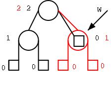
Why aren't we finished?
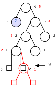
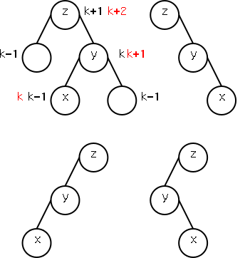
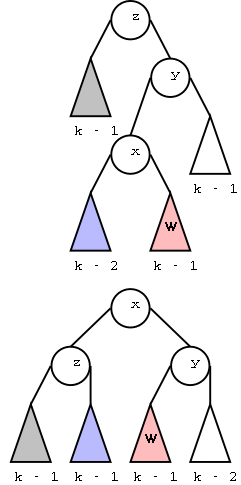 Let us consider the upper left double rotation, which is the rotation
that we need to apply the example above.
It is redrawn to the right with the subtrees drawn and their heights
labeled. The colors are so that you can see where they trees go when
we perform the rotation.
Let us consider the upper left double rotation, which is the rotation
that we need to apply the example above.
It is redrawn to the right with the subtrees drawn and their heights
labeled. The colors are so that you can see where they trees go when
we perform the rotation.
Recall that x is
an ancestor of w and has had its height raised from k-1 to k. The
sibling of x is at height k-1 and so is the sibling of y.
The reason x had its height raised is that one of its siblings (say
the right one) has been raised from k-2 to k-1.
How do I know the other one is k-2?
Ans: we will discuss it later.
The double rotation transforms the picture on top to the one on the bottom. We now actually are done with the insertion. Let's check the bottom picture and make sure.
Thus, if an insertion causes an imbalance, just one rotation re-balances the tree globally. We will see that for removals it is not this simple.
Answer to question posed above. One node was at height k-2 and its parent was at k-1. Hence the sibling was either at k-2 or k-3. But if it was at k-3, we would have found the tree out of balance when we got to x (x at k-1 after insertion, sibling at k-3). However, z is assumed to be the first time we found the tree out of balance starting from w (the insertion point) and moving up.
================ Start Lecture #20 ================
Here are the three pictures for the remaining three possibilities. That is, the other double rotation and both single rotations. The original configuration is shown on top and the result after the rotation is shown immediately below.
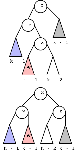
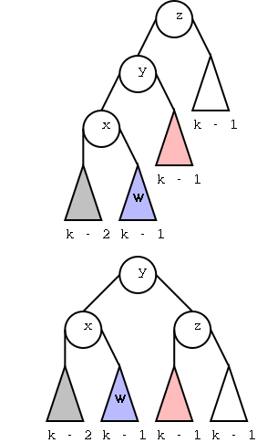
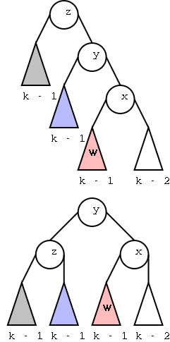
What is the complexity of insertion?
Hence we have the following
Theorem: The complexity of insertion in an AVL tree is Θ(log n).
Problem Set 3, problem 2. Please read the entire problem before beginning.
In order to remove an item with key k, we begin just as we did for an ordinary binary search tree. I repeat the procedure here.
The key concern is that we cannot simply remove an item from an internal node and leave a hole as this would make future searches fail. The beginning of the removal technique is familiar: w=TreeSearch(k,T.root()). If w is a leaf, k is not present, which we signal.
If w is internal, we have found k, but now the fun begins.
Returning the element with key k is easy, it is the element
stored in w.
We need to actually remove w, but we cannot leave a hole.
There are three cases.
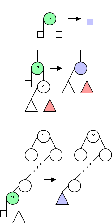
But now we have to possibly restore balance, i.e., maintain the AVL property. The possible trouble is that the light green node on the left has been replaced by the light blue on the right, which is of height one less. This might cause a problem. The sibling of the light green (not shown) might have height equal to, one less than, or one greater than, the light green.
To summarize the three cases either
In the second case we move up the tree and again have one of the same three cases so either.
The re-balancing is again a single or double rotation (since the problem is the same so is the solution).
The rotation will fix the problem but the result has a highest node whose height is one less the highest prior to the rotation (in the diagrams for single and double rotation the largest height dropped from k+2 to k+1).
Unlike the case for insertions this height reduction does not cancel out a previous height increase. Thus the lack of balance may continue to advance up the tree and more rotations may be needed.
Problem Set 3 problem 3 (end of problem set 3). Please read the entire problem before beginning.
What is the complexity of a removal? Remember that the height of an AVL tree is Θ(log(N)), where N is the number of nodes.
Theorem: The complexity of removal for an AVL tree is logarithmic in the size of the tree.
The news is good. Search, Inserting, and Removing all have logarithmic complexity.
The three operations all involve a sweep down the tree searching for a key, and possibly an up phase where heights are adjusted and rotations are performed. Since only a constant amount of work is performed per level and the height is logarithmic, the complexity is logarithmic.
================ Start Lecture #21 ================
Might come back to this if time permits.
We already did a sorting technique in chapter 2. Namely we inserted items into a priority queue and then removed the minimum each time. When we use a heap to implement the priority, the resulting sort is called heap-sort and is asymptotically optimal. That is, its complexity of O(Nlog(N)) is as fast as possible if we only use comparisons (proved in 4.2 below)
The idea is that if you divide an enemy into small pieces, each piece, and hence the enemy, can be conquered. When applied to computer problems divide-and-conquer involves three steps.
In order to prevent an infinite sequence of recursions, we need to define a stopping condition, i.e., a predicate that informs us when to stop dividing (because the problem is small enough to solve directly).
This turns out to be so easy that it is perhaps surprising that it is asymptotically optimal. The key observation is that merging two sorted lists is fast (the time is linear in the size of the list).
The steps are
Example:: Sort {22, 55, 33, 44, 11}.
Expanding the recursion one level gives.
Expanding again gives
Finally there still is one recursion to do so we get.
Hopefully there is a better way to describe this action. How about the following picture. The left tree shows the dividing. The right shows the result of the merging.
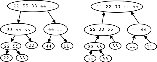
Definition: We call the above tree the merge-sort-tree.
In a merge-sort tree the left and right children of a node with A elements have ⌈A/2⌉ and ⌊A/2⌋ elements respectively.
Theorem: Let n be the size of the sequence to be sorted. If n is a power of 2, say n=2k, then the height of the merge-sort tree is log(n)=k. In general n = ⌈log(n)⌉.
Proof: The power of 2 case is part of problem set 4. I will do n=2k+1. When we divide the sequence into 2, the larger is ⌈n/2⌉=2k-1+1. When we keep dividing and look at the larger piece (i.e., go down the leftmost branch of the tree) we will eventually get to 3=21+1. We have divided by 2 k-1 times so are at depth k-1. But we have to go two more times (getting 2 and then 1) to get one element. So the depth is of this element is k+1 and hence the height is at least k+1.
The rest is part of problem set 2. Here is the idea. If you increase the number of elements in the root, you do not decrease the height. If n is not a power of 2, it is between two powers of 2 and hence the height is between the heights for these powers of two.
Problem Set 4, problem 1. Prove the theorem when n is a power of 2. Prove the theorem for n not a power of 2 either by finishing my argument or coming up with a new one.
The reason we need the theorem is that we will show that merge-sort spends time O(n) at each level of the tree and hence spends time O(n*height) in total. The theorem shows that this is O(nlog(n)).
This is quite clear. View each sequence as a deck of cards face up. Look at the top of each deck and take the smaller card. Keep going. When one deck runs out take all the cards from the other. This is clearly constant time per card and hence linear in the number of cards Θ(#cards).
Unfortunately this doesn't look quite so clear in pseudo code when we write it in terms of the ADT for sequences. Here is the algorithm essentially copied from the book. At least the comments are clear.
Algorithm merge(S1, S2, S):
   Input:  Sequences S1 and S2 sorted in nondecreasing order,
           and an empty sequence S
   Output: Sequence S contains the elements previously in S1 and S2
           sorted in nondecreasing order.  S1 and S2 now empty.

   {Keep taking smaller first  element until one sequence is empty}
   while (not(S1.isEmpty() or S2.isEmpty()) do
     if S1.first().element()<S2.first().element() then
        {move first element of S1 to end of S}
        S.insertLast(S1.remove(S1.first())
     else
        {move first element of S2 to end of S}
        S.insertLast(S2.remove(S2.first())

   {Now take the rest of the nonempty sequence.}
   {We simply take the rest of each sequence.}
   {Move the remaining elements of S1 to S
   while (not S1.isEmpty()) do
      S.insertLast(S1.remove(S1.first())
   {Move the remaining elements of S2 to S
   while (not S2.isEmpty()) do
      S.insertLast(S2.remove(S2.first())
Examining the code we see that each iteration of each loop removes an element from either S1 or S2. Hence the total number of iterations is S1.size()+S2.size(). Since each iteration requires constant time we get the following theorem.
Theorem: Merging two sorted sequences takes time
Θ(n+m), where n and m are the sizes of the two sequences.
The Running Time of Merge-Sort
We characterize the time in terms of the merge-sort tree. We assign to each node of the tree the time to do the divide and merge associated with that node and to invoke (but not to execute) the recursive calls. So we are essentially charging the node for the divide and combine steps, but not the solve recursively.
This does indeed account for all the time. Illustrate this with the example tree I drew at the beginning.
For the remainder of the analysis we assume that the size of the sequence to be sorted is n, which is a power of 2. It is easy to extend this to arbitrary n as we did for the theorem that is a part of problem set 4.
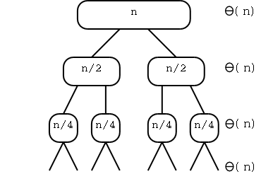 Now much time is charged to the root? The divide step takes time
proportional to the number of elements in S, which is n. The combine
step takes time proportional to the sum of the number of elements in
S1 and the number of elements in S1. But this is again n. So the
root node is charged Θ(n).
Now much time is charged to the root? The divide step takes time
proportional to the number of elements in S, which is n. The combine
step takes time proportional to the sum of the number of elements in
S1 and the number of elements in S1. But this is again n. So the
root node is charged Θ(n).
The same argument shows that any node is charged Θ(A), where A is the number of items in the node.
How much time is charged to a child of the root? Remember that we are assuming n is a power of 2. So each child has n/2 elements and is charged a constant times n/2. Since there are two children the entire level is charged Θ(n).
In this way we see that each level is Θ(n). Another way to see this is that the total number of elements in a level is always n and a constant amount of work is done on each.
Now we use the theorem saying that the height is log(n) to conclude that the total time is Θ(nlog(n)). So we have the following theorem.
Theorem: Merge-sort runs in Θ(nlog(n)).
Here is yet another way to see that the complexity is Θ(nlog(n)).
Let t(n) be the worst-case running time for merge-sort on n elements.
Remark: The worst case and the best case just differ by a multiplicative constant. There is no especially easy or hard case for merge-sort.
For simplicity assume n is a power of two. Then we have for some constants B and C
t(1) = B
t(n) = 2t(n/2)+Cn    if n>1
The first line is obvious the second just notes that to solve a problem we must solve 2 half-sized problems and then do work (merge) that is proportional to the size of the original problem.
If we apply the second line to itself we get
t(n) = 2t(n/2)+Cn = 2[2t(n/4)+C(n/2)]+Cn =
22t(n/22)+2Cn
If we apply this i times we get
t(n) = 2it(n/2i)+iCn
When should we stop?
Ans: when we get to the base case t(1). This occurs when
2i=n, i.e. when i=log(n).
t(n)   =  2log(n)t(n/2log(n)) + log(n)Cn
       =  nt(n/n) + log(n)Cn               since 2log(n)=n
       =  nt(1) + log(n)Cn
       =  nB + Cnlog(n)
which again shows that t(n) is Θ(nlog(n)).
================ Start Lecture #22 ================
Skipped for now
It is interesting to compare quick-sort with merge-sort. Both are divide and conquer algorithms. So we divide, recursively sort each piece, and then combine the sorted pieces.
In merge-sort, the divide is trivial: throw half the elements into one pile and the other half in another pile. The combine step, while easy does do comparisons and picks an element from the correct pile.
In quick-sort, the combine is trivial: pick up one pile, then the other. The divide uses comparisons to decide which pile each element should be placed into.
As usual we assume that the sequence we wish to sort contains no duplicates. It is easy to drop this condition if desired.
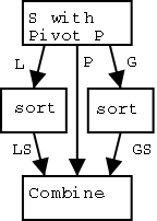
Algorithm quick-sort (S)
   Input: A sequence S (of size N).
   Output: A sorted sequence T containing
           the same elements as S.

   Create a empty sequences T, L, G

   { Divide into L and G }
   If n = 1
      then copy the element of S to T
   if n < 2
      return
   Pick an element P from S { called the pivot }
   while (not S.isEmpty())
      x ← S.remove(S.first())
      if x < P then
         L.insertLast(x)    { L stands for less }
      if x > P then
         G.insertLast(x)    { G stands for greater }

   { Recursively Sort L and G }
   LS ← quick-sort (L)    LS stands for L sorted }
   GS ← quick-sort (G)

   { Combine LS, P, and GS }
   while (not LS.isEmpty())
      T.insertLast(LS.remove(LS.first()))
   T.insertLast(P)
   while (not GS.isEmpty())
      T.insertLast(GS.remove(GS.first()))
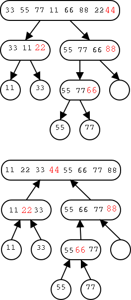 The running time of quick sort is highly dependent on the choice of
the pivots at each stage of the recursion.
A very simple method is to choose the last element as the pivot.
This method is illustrated in the figure on the right. The pivot is
shown in red. This tree is not surprisingly called the
quick-sort tree.
The running time of quick sort is highly dependent on the choice of
the pivots at each stage of the recursion.
A very simple method is to choose the last element as the pivot.
This method is illustrated in the figure on the right. The pivot is
shown in red. This tree is not surprisingly called the
quick-sort tree.
The top tree shows the dividing and recursing that occurs with input {33,55,77,11,66,88,22,44}. The tree below shows the combining steps for the same input.
As with merge sort, we assign to each node of the tree the cost (i.e., running time) of the divide and combine steps. We also assign to the node the cost of the two recursive calls, but not their execution. How large are these costs?
The two recursive calls (not including the subroutine execution itself) are trivial and cost Θ(1).
The dividing phase is a simple loop whose running time is linear in the number of elements divided, i.e., in the size of the input sequence to the node. In the diagram this is the number of numbers inside the oval.
Similarly, the combining phase just does a constant amount of work per element and hence is again proportional to the number of elements in the node.
We would like to make an argument something like this. At each level of each of the trees the total number of elements is n so the cost per level is O(n). The pivot divides the list in half so the size of the largest node is divided by two each level. Hence the number of levels, i.e., the height of the tree, is O(log(n)). Hence the entire running time is O(nlog(n)).
That argument sound pretty good and perhaps we should try to make it more formal. However, I prefer to try something else since the argument is WRONG!
Homework:
Draw the quick-sort
tree for sorting the following sequence
{222 55 88 99 77 444 11 44 22 33 66 111 333}.
Assume the pivot is always the last element.
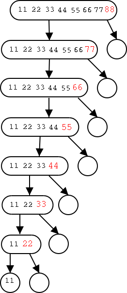 The tree on the right illustrates the worst case of quick-sort, which
occurs when the input is already sorted!
The tree on the right illustrates the worst case of quick-sort, which
occurs when the input is already sorted!
The height of the tree is N-1 not O(log(n)). This is because the pivot is in this case the largest element and hence does not come close to dividing the input into two pieces each about half the input size.
It is easy to see that we have the worst case. Since the pivot does not appear in the children, at least one element from level i does not appear in level i+1 so at level N-1 you can have at most 1 element left. So we have the highest tree possible. Note also that level i has at least i pivots missing so cna have at most N-i elements in all the nodes. Our tree achieves this maximum. So the time needed is proportional to the total number of numbers written in the diagram which is N + N-1 + N-2 + ... + 1, which is again the one summation we know N(N+1)/2 or Θ(N2.
Hence the worst case complexity of quick-sort is quadratic! Why don't we call it slow sort?
Perhaps the problem was in choosing the last element as the pivot. Clearly choosing the first element is no better; the same example on the right again illustrates the worst case (the tree has its empty nodes on the left this time).
Since are spending linear time (as opposed to constant time) on the division step, why not count how many elements are present (say k) and choose element number k/2? This would not change the complexity (it is also linear). You could do that and now a sorted list is not the worst case. But some other list is. Just put the largest element in the middle and then put the second largest element in the middle of the node on level 1. This does have the advantage that if you mistakenly run quick-sort on a sorted list, you won't hit the worst case. But the worst case is still there and it is still Θ(N2).
Why not choose the real middle element as the pivot, i.e., the median. That would work! It would cut the sizes in half as desired. But how do we find the median? We could sort, but that is the original problem. In fact there is a (difficult) algorithm for computing the median in linear time and if this is used for the pivot, quick-sort does take O(nlog(n)) time in the worst case. However, the difficult median algorithm is not fast in practice. That is, the constants hidden in saying it is Θ(N) are rather large.
Instead of studying the fast, difficult median algorithm, we will consider a randomized quick-sort algorithm and show that the expected running time is Θ(Nlog(N)).
Problem Set 4, Problem 2.
Find a sequence of size N=12 giving the worst case for quick-sort when
the pivot for sorting k elements is element number ⌊k/2⌋.
Consider running the following quick-sort-like experiment.
Are good splits rare or common?
Theorem: (From probability theory). The expected number of times that a fair coin must be flipped until it shows ``heads'' k times is 2k.
We will not prove this theorem, but will apply it to analyze good
splits.
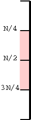
We picked the pivot at random so if we imagine the N numbers lined up in order, the pivot is equally likely to be anywhere in this line.
Consider the picture on the right. If the pivot is anywhere in the pink, the split is good. But the pink is half the line so the probability that we get a ``pink pivot'' (i.e., a good split) is 1/2. This is the same probability that a fair coin comes up heads.
Every good split divides the size of the node by at least 4/3. Recall that if you divide N by 4/3, log4/3(N) times, you will get 1. So the maximum number of good splits possible along a path from the root to a leaf is log4/3(N).
Apply the probability theorem above we see that the expected length of a path from the root to a leaf is at most 2log4/3(N), which is O(log(N)). That is, the expected height is O(log(N)).
Since the time spent at each level is O(N), the expected running time of randomized quick-sort is O(Nlog(N)).
Theorem: The running time of any comparison-based sorting algorithm is Ω(Nlog(N)).
Proof: We will not cover this officially.
Unofficially the idea we form a binary tree with each node
corresponding to a comparison and the two children corresponding to
the two possible outcomes. This is a tree of all possible executions
(with only comparisons used for decisions). There are N! permutations
of N numbers and each must give a different execution pattern in order
to be sorted. So there are at least N! leaves. Hence the height is
at least log(N!). But N! has N/2 elements that are at least N/2 so
N!≥(N/2)N/2. Hence
height ≥ log(N!) ≥ log((N/2)N/2) = (N/2)log(N/2)
So the running time, which is at least the height of this tree, is
Ω(Nlog(N))
Corollary: Heap-sort, merge-sort, and quick sort (with the difficult, linear-time median algorithm) are asymptotically optimal.
================ Start Lecture #23 ================
We have seen that the fastest comparison-based sorting algorithms run in time Θ(Nlog(N)), where N is the number of items to sort. In this section we are going to develop faster algorithms. Hence they must not be comparison-based algorithms.
We make a key assumption, we are sorting items whose keys are integers in a bounded range [0, R-1].
Question: Let's start with a special case R=N so we are sorting N items with integer keys from 0 to N-1. As usual we assume there are no duplicate keys. Also as usual we remark that it is easy to lift this restriction. How should we do this sort?
Answer: That was a trick question. You don't even have to look at the input. If you tell me to sort 10 integers in the range 0...9 and there are no duplicates, I know the answer is {0,1,2,3,4,5,6,7,8,9}. Why? Because, if there are no duplicates, the input must consist of one copy of each integer from 0 to 10.
OK, let's drop the assumption that R=N. So we have N items (k,e),
with each k an integer, no duplicate ks, and 0≤k<R. The trick is
that we can use k to decide where to (temporarily) store e.
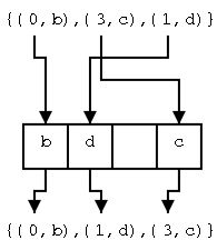
Algorithm preBucketSort(S)
   input:  A sequence S of N items with integer keys in range [0,N)
   output: Sequence S sorted in increasing order of the keys.

   let B be a vector of R elements,
       each initially a special marker indicating empty

   while (not S.isEmpty())
      (k,e) ← S.remove(S.first())
      B[k] ← e         <==== the key idea (not a comparison)

   for i ← 0 to R-1 do
      if (B[i] not special marker) then
         S.insertLast((i,B[i])
To convert this algorithm into bucket sort we drop the artificial
assumption that there are not duplicates. Now instead of a vector of
items we need a vector of buckets, where a bucket is a sequence of
items.
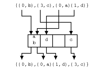
Algorithm BucketSort(S)
   input:  A sequence S of N items with integer keys in range [0,N)
   output: Sequence S sorted in increasing order of the keys.

   let B be a vector of R sequences of items
       each initially  empty

   while (not S.isEmpty())
      (k,e) ← S.remove(S.first())
      B[k].insertLast(e)      <==== the key idea

   for i ← 0 to R-1 do
      while (not B[i].isEmpty())
         S.insertLast((i,B[i].remove(B[i].first())))
The first loop has N iterations each of which run in time Θ(1), so the loop requires time Θ(N). The for loop has R iterations so the while statement is executed R times. Each while statement requires time Θ(1) (excluding the body of the while) so all of them require time Θ(N) The total number of iterations of all the inner while loops is again N and each again requires time Θ(1), so the time for all inner iterations is Θ(N).
The previous paragraph shows that the complexity is Θ(N)+Θ(R) = Θ(N+R).
So bucket-sort is a winner if R is not too big. For example if R=O(N), then bucket-sort requires time only Θ(N). Indeed if R=o(Nlog(N)), bucket-sort is (asymptotically) faster than any comparison based sorting algorithm (using worst case analysis).
Definition: We call a sort stable if equal elements remain in the same relative position. Stated more formally: for any two items (ki,ei) and (kj,ej) such that item (ki,ei) precedes item (kj,ej) in S (i.e., i<j), then item (ki,ei) precedes item (kj,ej) after sorting as well.
Stability is often convenient and will prove so in the next section on radix-sort. We note that bucket-sort is stable since we treated each bucket in a fifo manner inserting at the rear and removing from the front.
Let's extend our sorting study from integer keys to keys that are themselves pairs of integers. The first question to ask is, given two keys (k,m) and (k',m'), which is larger? Note that (k,m) is just the key; an item would be written ((k,m),e).
Definition: The lexicographical (dictionary) ordering on pairs of integers is defined by declaring (k,m) < (k',m') if either
Note that this really is dictionary order:
canary < eagle < egret < heron
Algorithm radix-sort-on-pairs
   input:  A sequence S of N items with keys
           pairs of integers in the range [0,N)
           Write elements of S as ((k,m),e)
   output: Sequence S lexicographically sorted on the keys

   bucket-sort(S) using m as the key
   bucket-sort(S) using k as the key
Do an example of radix sorting on pairs and then do it incorrectly, by reversing the order of the bucket sorts.
What if the keys are triples or in general d-tuples?
The answer is ...
Homework: R-4.15
Theorem: Let S be a sequence of N items each of which has a key (k1,k2,...kd), where ki is in integer in the range [0,R). We can sort S lexicographically in time O(n(N+R)) using radix-sort.
Insertion sort or bubble sort are not suitable for general sorting of large problems because their running time is quadratic in N, the number of items. For small problems, when time is not an issue, these are attractive because they are so simple. Also if the input is almost sorted, insertion sort is fast since it can be implemented in a way that is O(N+A), where A is the number of inversions, (i.e., the number of pairs out of order).
Heap-sort is a fine general-purpose sort with complexity Θ(Nlog(N)), which is optimal for comparison-based sorting. Also heap-sort can be executed in place (i.e., without much extra memory beyond the data to be sorted). (The coverage of in-place sorting was ``unofficial'' in this course.) If the in-place version of heap-sort fits in memory (i.e., if the data is less than the size of memory), heap-sort is very good.
Merge-sort is another optimal Θ(Nlog(N)) sort. It is not easy to do in place so is inferior for problems that can fit in memory. However, it is quite good when the problem must be do ``out-of-core'' since it doesn't fit. We didn't discuss this issue, but the merges can be done with two input and one output file (this is not trivial to do well, you want to utilize the available memory in the most efficient manner).
Quick-sort is hard to evaluate. The version with the fast median algorithm is fine theoretically (worst case again Θ(Nlog(N)) but not used because of large constant factors in the fast median. Randomized quick-sort has a low expected time but a poor worst-case time. It can be done in place and is quite fast in that case, often the fastest. But the quadratic worst case is a fear (and a non-starter for many real-time applications).
Bucket and radix sort are wonderful when they apply, i.e., when the keys are integers in a modest range (R a small multiple of N). For radix sort with d-tuples the complexity is Θ(d(N+R)) so if d(N+R) is o(Nlog(N)), radix sort is asymptotically faster than any comparison based sort (e.g., heap-, insertion-, merge-, or quick-sort).
Selection means the ability to find the kth smallest element. Sorting will do it, but there are faster (comparison-based) methods. One example problem is finding the median (N/2 th smallest).
It is not too hard (but not easy) to implement selection with linear expected time. The surprising and difficult result is that there is a version with linear worst-case time.
================ Start Lecture #24 ================
The greedy method is applied to maximization/minimization problems. The idea is to at each decision point choose the configuration that maximizes/minimizes the objective function so far. Clearly this does not lead to the global max/min for all problems, but it does for a number of problems.
This chapter does not make a good case for the greedy method. since it is used to solve simple cases of standard problems in which the more normal cases do not use the greedy method. However, there are better examples, for example minimal the spanning tree and shortest path graph problems. The two algorithms chosen for this section, fractional knapsack and task scheduling, were (presumably) chosen because they are simple and natural to solve with the greedy method.
In the knapsack problem we have a knapsack of a fixed capacity (say W pounds) and different items i each with a given weight wi and a given benefit bi. We want to put items into the knapsack so as to maximize the benefit subject to the constraint that the sum of the weights must be less than W.
The knapsack problem is actually rather difficult in the normal case where one must either put an item in the knapsack or not. However, in this section, in order to illustrate greedy algorithms, we consider a much simpler variation in which we can take part of an item and get a proportional part of the benefit. This is called the ``fractional knapsack problem'' since we can take a fraction of an item. (The more common knapsack problem is called the ``0-1 knapsack problem'' since we either take all (1) or none (0) of an item.
In symbols, for each item i we choose an amount xi (0≤xi≤wi) that we will place in the knapsack. We are subject to the constraint that the sum of the xi is no more than W since that is all the knapsack can hold.
We again desire to maximize the total benefit. Since, for item i, we only put xi in the knapsack, we don't get the full benefit. Specifically we get benefit (xi/wi)bi.
But now this is easy!
Why doesn't this work for the normal knapsack problem when we must take all of an item or none of it?
algorithm FractionalKnapsack(S,W):
   Input:  Set S of items i with weight wi and benefit bi all positive.
           Knapsack capacity W>0.
   Output: Amount xi of i that maximizes the total benefit without
           exceeding the capacity.

   for each i in S do
      xi ← 0        { for items not chosen in next phase }
      vi ← bi/wi    { the value of item i "per pound" }
   w ← W            { remaining capacity in knapsack }

   while w > 0 do
      remove from S an item of maximal value   { greedy choice }
      xi ← min(wi,w)  { can't carry more than w more }
      w ← w-xi
FractionalKnapsack has time complexity O(NlogN) where N is the number of items in S.
Homework: R-5.1
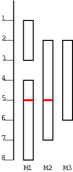
We again consider an easy case of a well known optimization problem.
In the figure there are 6 tasks, with start times and finishing times (1,3), (2,5), (2,6), (4,5), (5,8), (5,7). They are scheduled on three machines M1, M2, M3. Clearly 3 machines are needed as can be seen by looking at time 4.
In our greedy algorithm we only go to a new machine when we find a task that cannot be scheduled on the current machines.
Algorithm TaskSchedule(T):
   Input:  A set T of tasks, each with start time si and finishing time fi
           (si≤fi).
   Output: A schedule of the tasks of T on the minimum number of machines.

   m ← 0                                   { current number of machines }
   while T is not empty do
      remove from T a task i with smallest start time
      if there is an Mj having all tasks non-conflicting with i then
         schedule i on Mj
      else
         m ← m+1
         schedule i on Mm
Assume the algorithm runs and declares m to be the minimum number of machines needed. We must show that m are really needed.
The book asserts that it is easy to see that the algorithm runs in time O(NlogN), but I don't think this is so easy. It is easy to see O(N2).
Homework: R-5.3
Problem Set 4, Problem 3.
Part A. C-5.3 (Do not argue why your algorithm is correct).
Part B. C-5.4.
Remark: Problem set 4 is now assigned and due 4 Dec 02.
================ Start Lecture #25 ================
The idea of divide and conquer is that we solve a large problem by solving a number of smaller problems and then we apply this idea recursively.
From the description above we see that the complexity of a divide and conquer solution has three parts.
Let T(N) be the time required to solve an instance of the problem having time N. The time required to split the problem and combine the subproblems is typically a function of N, say f(N).
More interesting is the time required to solve the subproblems. If the problem has been split in half then the time required for each subproblem is T(N/2).
Since the total time required includes splitting, solving both subproblems, and combining we get.
T(N) = 2T(N/2)+f(N)
Very often the splitting and combining are fast, specifically linear in N. Then we get
T(N) = 2T(N/2)+bN
for some constant b. (We probably should say ≤ rather than =, but
we will soon be using big-Oh and friends so we can afford to be a
little sloppy.
What if N is not divisible by 2? We should be using floor or ceiling or something, but we won't. Instead we will be assuming for recurrences like this one that N is a power of two so that we can keep dividing by 2 and get an integer. (The general case is not more difficult; but is more tedious)
But that is crazy! There is no integer that can be divided by 2 forever and still give an integer! At some point we will get to 1, the so called base case. But when N=1, the problem is almost always trivial and has a O(1) solution. So we write either
           b              if N = 1
    T(N) =
           2T(N/2)+bN   if N > 1
or
    T(1) = b
    T(N) = 2T(N/2)+bN   if N > 1
No we will now see three techniques that, when cleverly applied, can solve a number of problems. We will also see a theorem that, when its conditions are met, gives a solution without our being clever.
Also called ``plug and chug'' since we plug the equation into itself and chug along.
    T(N) = 2T(N/2)+bN
         = 2[    ]+bN
         = 2[2T((N/2)/2)+b(N/2)]+bN
         = 4T(N/4)+2bN    now do it again
         = 8T(N/8)+3bN
A flash of inspiration is now needed. When the smoke clears we get
T(N) = 2iT(N/2i)+ibN
When i=log(N), N/2i=1 and we have the base case. This gives the final result
    T(N) = 2log(N)T(N/2log(N))+ibN
         = N    T(1)      +log(N)bN
         = Nb +log(N)bN
Hence T(N) is O(Nlog(N))
The idea is similar but we use a visual approach.
We already studied the recursion tree when we analyzed merge-sort. Let's look at it again.
The diagram shows the various subproblems that are executed, with their sizes. (It is not always true that we can divide the problem so evenly as shown.) Then we show that the splitting and combining that occur at each node (plus calling the recursive routine) only take time linear in the number of elements. For each level of the tree the number of elements is N so the time for all the nodes on that level is Θ(N) and we need to find the height of the tree. When the tree is split so evenly the sizes of all the nodes on each level go down by a factor of two so we reach a node with size 1 in logN levels (assuming N is a power of 2). Thus T(N) is Θ(Nlog(N)).
This method is really only useful after you have practice in recurrences. The idea is that, when confronted with a new problem, you recognize that it is similar to a problem you have seen the solution to previously and you guess that the solution to the new problem is similar to the old.
But we don't have enough experience for this to be very useful.
In this section, we apply the heavy artillery. The following theorem, which we will not prove, enables us to solve some problems by just plugging in.
We will only be considering complexities of the form
    T(1) = c
    T(N) = aT(N/b)+f(N)   if N > 1
The idea is that we have done some sort of divide and conquer where there are a subproblems of size at most N/b. As mentioned earlier f(N) accounts for the time to divide the problem into subproblems and to combine the subproblem solutions.
Theorem [The Master Theorem]: Let f(N) and T(N) be as above.
Proof: Not given.
Remarks:
Now we can solve some problems easily and will do two serious problems after that.
Example: T(N) = 4T(N/2)+N.
Example: T(N) = 2T(N/2) = Nlog(N)
Example: T(N) = T(N/4) + 2N
Example: T(N) = 9T(N/3) + N2.5
Homework: R-5.4
We want to multiply big integers.
When we multiply without machine help, we use as knowledge the times tables for all 1 digit numbers and then do the standard 5th-grade algorithm that requires Θ(N2) steps for N digit numbers. On a computer the known tables are for all 32-bit numbers (or 64-bit on some machines). If we want to multiply two 32N-bit numbers on the computer we could write the 5-th grade algorithm in software (using 32-bit numbers as ``digits'') and again compute the result in Θ(N2) time.
To make the wording easier lets assume we only know how to multiply 1-bit numbers and we want to multiply two N-bit numbers X and Y. Using the 5th grade algorithm we can do this in time Θ(N2). We want to go faster.
If we simply divide the bits in half (the high order and the low order), we see that to multiply X and Y we need to compute 4 sub-products Xhi*Yhi+Xhi*Ylo+Xlo*Yhi+Xlo*Ylo. (Note that when I write the products above I don't include the powers of 2 needed. This corresponds to writing the numbers in the correct column with the 5th grade algorithm.)
Since addition of K-bit numbers is Θ(K) and our multiplications are only of N/2-bit values we get
T(N) = 4T(N/2)+cnBut when we apply the master theorem (case 1) we just get T(N)=N2, which is no improvement. We try again and with cleverness are able to get by with three instead of four multiplications.
We compute Xhi*Yhi, Xlo*Ylo, and the miraculous (Xhi-Xlo)*(Ylo-Yhi). The miracle multiplication produces the two remaining terms we need but has added to this two other terms. But those are just the (negative of) the two terms we did compute so we can add them back and they cancel.
The summary is that T(N) = 3T(N/2)+cN, which by the master theorem (case 1) gives T(N) is Θ(Nlog23N). But log23<1.585 so we get the surprising
Theorem: We can multiple two N-bit numbers in O(N1.585) time.
If you thought the integer multiplication involved pulling a rabbit out of our hat, get ready.
This algorithm was a sensation when it was discovered by Strassen. The standard algorithm for multiply two NxN matrices is Θ(N3). We want to do better
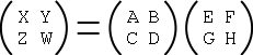 First try. Assume N is a power of 2 and break each matrix into 4
parts as shown on the right. Then X = AE+BG and similarly for Y, Z,
and W. This gives 8 multiplications of half size matrices plus
Θ(N2) scalar addition so
First try. Assume N is a power of 2 and break each matrix into 4
parts as shown on the right. Then X = AE+BG and similarly for Y, Z,
and W. This gives 8 multiplications of half size matrices plus
Θ(N2) scalar addition so
T(N) = 8T(N/2) + bN2
We apply the master theorem and get T(N) = Θ(N3),
i.e., no improvement.
But strassen found the way! He (somehow, I don't know how) decided to consider the following 7 (not 8) multiplications of half size matrices.
S1 = A(F-H)       S2 = (A+B)H       S3 = (C+D)E       S4 = D(G-E)
S5 = (A+D)(E+H)   S6 = (B-D)(G+H)   S7 = (A-C)(E+F)
Now we can compute X, Y, Z, and W from the S's
X = S5+S6+S4-S2 Y = S1+S2 Z = S3+S4 W = S1-S7-S3+S5
This computation shows that
T(N) = 7T(N/2) + bN2
Thus the master theorem now gives
Theorem(Strassen): We can multiply two NxN matrices in time O(nlog7).
Remarks:
================ Start Lecture #26 ================
This is a little hard to explain abstractly.
One idea is that we compute a max by maximizing over a bunch of smaller possibilities (and apply this recursively). We then compute these maxima backwards. That is, instead of breaking the big one into small ones, we start with the small ones.
Another idea is that we save many intermediate results since they will be reused. So we really should analyze the space complexity as well as the time complexity.
In this problem we want to multiple n matrices
A0 * A1 * ... * An-1
Unlike the matrix multiplication from last lecture, these matrices are not all of the same size. But to be able to multiply the matrices, the number of columns in Ai must be the same as the number of rows in the next matrix Ai+1. Specifically Ai is of size di by di+1.
Matrix multiplication is associative, that is
X * (Y * Z) = (X * Y) * Z
Hence in computing the matrix chain-product above, we can do the
multiplications is any order we want and get the same answer. Perhaps
surprisingly, some orders are much faster than others.
Example: Consider A * B * C where
A is a 20x60 matrix
B is a 60x50 matrix
C is a 50x10 matrix
First we perform the computation as A * (B * C).
B * C requires 50 multiplications for each entry in the output. Since the output is 60x10, there are 600 entries and hence 30,000 multiplications are required to produce the 60x10 result.
We now must multiple A by this new 60x10 matrix. This matrix product requires 60 multiplications for each entry in the output. Since the output is 20x10, there are 200 entries and hence 12,000 multiplications are required. So the overall computation requires 42,000 multiplications.
Now we perform the computation as (A * B) * C.
A * B requires 60 multiplications for each entry. Since the output is 20x50, there are 1000 entries and hence 60,000 multiplications. We now multiply this result by C. This matrix product requires 50 multiplications for each entry. Since the output is 20x10, there are 200 entries and hence 10,000 multiplications are required. So the overall computation requires 70,000 multiplication.
 Example:
Do on the board the example on the right. Notice that the answers are
the same for either order of parenthesizing but that the numbers of
multiplications are different.
Example:
Do on the board the example on the right. Notice that the answers are
the same for either order of parenthesizing but that the numbers of
multiplications are different.
The matrix chain-product problem is to determine the parenthesization that minimizes the number of multiplications.
(Obvious) solution. Try every parenthesization and pick the best one.
The obvious solution, often called the brute force solution, has exponential complexity since the number of ways to parenthesize an associative expression with n terms is the nth so-called Catalan number, which is Ω(4n/n3/2).
We want to do better and will do so using dynamic programming. We need to define subproblems, subsubproblems, etc and then compute the answer backwards taking advantage of common subproblems, the solutions to which we store.
Recall that the matrix product whose multiplications we are trying to minimize is
A0 * ... * An-1We want an convenient notation to describe various subproblems and define Ni,j to be the minimum number of multiplications needed to compute the subexpression
Ai * ... * AjIn particular N0,n-1 is the original problem.
What follows is the key point of dynamic programming.
The key observation about matrix chain-product is that we can characterize the optimal solution in terms of optimal solutions of the subproblems. (The book calls this the subproblem optimality condition.)
We note specifically that when computing Ai*...*Aj there must be a last matrix multiplication so that
Ai*...*Aj = (Ai*...*Ak)*(Ak+1*...*Aj)and (the KEY point) to get the minimum number of multiplications for Ai*...*Aj we must have the minimum number of multiplications for Ai*...*Ak and for Ak+1*...Aj. This says that Ni,j is just the minimum over all possible k's of
What is the cost of the final matrix multiplication?
We have just seen that
Ni,j = mini≤k<j {Ni,k + Nk+1,j + didk+1dj+1}
Let's call this the fundamental equation.
Although the fundamental equation does not look simple, let's not be discouraged and keep going. First of all if we apply this recursively we will get terms in which the subscripts of N are close together. We can stop the recursion when the subscripts are equal since Ni,i=0 because no multiplications are required since no matrix product is being computed.
Remember that the idea of dynamic programming is to run the recursion backwards and start with the smallest problems.
algorithm MatrixChain(d0,...,dn) (dynamic programming)
   Input:  Sequence d0,...,dn of positive integer
           corresponding to the dimensions of a chain of matrices
           A0,...,An-1
   Output: Ni,j, the minimum number of multiplications
           needed to compute Ai*...*Aj

   for i ← 0 to n-1 do           { the simple base case }
      Ni,i ← 0

   for b ← 1 to n-1 do           { keep doing larger gaps }
      for i ← 0 to n-1-b         { to keep j in bounds )
         j ← i+b
         { Calculate Ni,j from the fundamental equation }
         Ni,j ← +infinity
         for k ← i to j-1 do
            Ni,j ← min(Ni,j,Ni,k+Nk+1,j+didk+1dj+1)
This algorithm calculates the minimum number of parenthesis needed for any contiguous subset of the matrices. In particular N0,n-1 gives the minimum number of parenthesis needed for the entire matrix chain-product.
Example: Compute, on the board, the minimum number of multiplications needed for the example drawn previous. We have three matrices of shape 2x2, 2x2 and 2x1 respectively so n=3 and the d vector is 2,2,2,1.
Homework: R-5.9
This is easy now that we know the algorithm.
The algorithm clearly takes O(n3) time since it has a triply nested loop and each loop has O(n) iterations.
But the algorithm gives the number of parentheses not where they should be placed. We can fix this problem by storing in Ni,j not just the number of parentheses but the index k that gave us the solution.
Theorem: We can compute a parenthesization that minimizes the number of multiplications in a matrix chain-product in O(n) time, where n is the number of matrices.
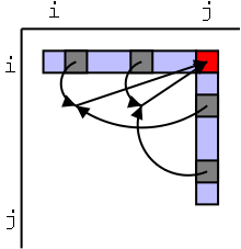 The diagram on the right illustrates the way dynamic program generates
the elements of N.
The diagram on the right illustrates the way dynamic program generates
the elements of N.
Remark: The space complexity is Θ(N2) since the only storage used is the array N (plus a few scalars).
There are three properties needed for successful application of dynamic programming.
This is the real knapsack problem, a well-known NP-complete problem. So clearly we will not get a polynomial time solution (but we will get close).
Consider a knapsack that can hold a maximum capacity W and a set S of n items with item i weighing wi and giving benefit bi. All the w's, b's and W are positive integers.
The problem is to maximize the benefit of the items carried subject to the constraint that the total weight cannot exceed W. It is called the 0-1 knapsack problem because, for each item, you leave it behind (0) or take all of it (1). You cannot choose to take for example half of the item as you could in the fractional knapsack problem discussed at the beginning of this chapter.
Homework: R-5.12
Let Si consist of items 1,2,...,i. So Sn is all of S. The idea is that subproblem k will be to find the optimal way to load the knapsack using only items in Sk, i.e., items 1,...,k. Then the overall answer is obtained by solving Sn.
It is indeed possible to split the problem this way and when split enough we get S1, which is trivial to optimize since there is only one element.
There is subproblem overlap as desired.
But it is not at all clear how to extend an optimal solution found for Sk to an optimal solution for Sk+1. Indeed finding the optimal solution for S1, then S2, then S3, corresponds to deciding on each element one at a time. This would be a greedy solution and doesn't give a global optimal.
One could also define Si,j, analogous to Ni,j above. However, we again don't have a way to extend an optimal solutions to subproblems into an optimal solution for a bigger subproblem.
The problem is that by defining the subproblem simply in terms of k, we do not get enough information to construct a solution that is helpful to obtaining a global maximum.
Instead we define subproblems in a more complicated manner. This is a stroke of inspiration and is not at all obvious.
Let B[k,w] be the maximum benefit obtainable from items in Sk having total weight exactly w. Our overall goal is to find B[n,W], the original 0-1 knapsack problem.
This does split the problems into subproblems and when we get down to B[0,w] we have an trivial problem with solution 0 since we have no items to select from. (Also B[k,0] is zero since we are not permitted to choose any items since our weight limit is 0, but we don't use this fact.)
The key that makes this solution work is the observation that
        /      B[k-1,w]                   if wk>w
B[k,w] =
        \ max {B[k-1,w], B[k-1,w-wk]+bk}   otherwise
This looks formidable, but is not. We need to choose a subset of the first k items with weight exactly w. If the kth item weighs more than w, it cannot be used so the best we can do with the first k items is the same as the best we can do with the first k-1 items. That was the easier case.
If the kth item is not heavier than w, it can be used, but need not be (that gives the two possibilities in the max). If we choose not to use the kth item, we get the previous case (the first term in the max). If we use the kth item and get total weight w, the items chosen from the first k-1 must weight w-wk. Also in this case we gain the benefit of the kth item.
This looks pretty good. We can loop on k and inside that on w. B[k,*] just depends on B[k-1,*] so it works fine.
Algorithm 01knapsack(S,W)
   Input:  A set S of n items each with weight wi and benefit bi.
           A max weight W.  All are positive; all weights integers.
   Output: B[k,w] the maximum benefit obtainable from a subset of
           the first k items in S having total weight w.

   for w ← 0 to W          { base case }
      B[0,w] ← 0

   for k ← 1 to n
      for w ← 0 to W
         if wk > w then
            B[k,w] ← B[k-1,w]
         else
            B[k,w] =  max (B[k-1,w], B[k-1,w-wk]+bk)
This is easy, each loop iteration is constant time so the complexity is the number of iterations. The base case loop has Θ(W) iterations and the nested loops have Θ(nW).
Theorem: Given a positive integer W and a set S of n items each with positive benefit and positive integer weight, we can find the highest benefit subset of S with total weight at most W in time Θ(nW).
Remarks:
End of Remarks
At first glance the theorem above seems to say that there is a polynomial time solution to the 0-1 knapsack problem. The time complexity is Θ(nW), the product of two numbers characteristic of the input. But this is wrong!
The definition of polynomial time is that the algorithm takes time that is polynomial in the size of the input. What is the size of the input?
Remark: It is common to refer to algorithms like ours as requiring pseudo-polynomial time. That is it is polynomial the value of a number in the input, but not on its input size (the size of its binary representation).