Operating Systems
Chapter 2: Process Management
Tanenbaum's chapter title is ``processes''. I prefer process
management. The subject matter is processes, process scheduling,
interrupt handling, and IPC (Interprocess communication--and
coordination).
2.1: Processes
Definition: A process is a program
in execution.
- We are assuming a multiprogramming OS that
can switch from one process to another.
- Sometimes this is
called pseudoparallelism since one has the illusion of a
parallel processor.
- The other possibility is real
parallelism in which two or more processes are actually running
at once because the computer system is a parallel processor, i.e., has
more than one processor.
- We do not study real parallelism (parallel
processing, distributed systems, multiprocessors, etc) in this course.
2.1.1: The Process Model
Even though in actuality there are many processes running at once, the
OS gives each process the illusion that it is running alone.
Virtual time and virtual memory are examples of abstractions
provided by the operating system to the user processes so that the
latter ``sees'' a more pleasant virtual machine than actually exists.
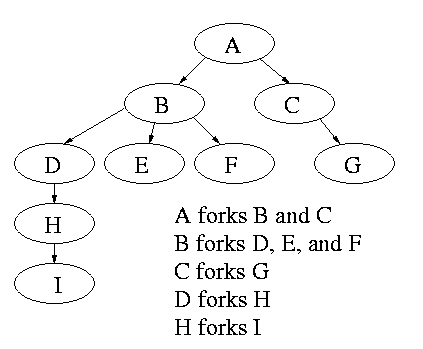
Process Hierarchies
Modern general purpose operating systems permit a user to create and
destroy processes.
- In unix this is done by the fork
system call, which creates a child process, and the
exit system call, which terminates the current
process.
- After a fork both parent and child keep running (indeed they
have the same program text) and each can fork off other
processes.
- A process tree results. The root of the tree is a special
process created by the OS during startup.
- A process can choose to wait for children to terminate.
For example, if C issued a wait() system call it would block until G
finished.
Old or primitive operating system like
MS-DOS are not multiprogrammed so when one process starts another,
the first process is automatically blocked and waits until
the second is finished.
Process states and transitions
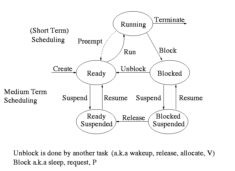
The above diagram contains a great deal of information.
- Consider a running process P that issues an I/O request
- The process blocks
- At some later point, a disk interrupt occurs and the driver
detects that P's request is satisfied.
- P is unblocked, i.e. is moved from blocked to ready
- At some later time the operating system looks for a ready job
to run and picks P.
- A preemptive scheduler has the dotted line preempt;
A non-preemptive scheduler doesn't.
- The number of processes changes only for two arcs: create and
terminate.
- Suspend and resume are medium term scheduling
- Done on a longer time scale.
- Involves memory management as well.
- Sometimes called two level scheduling.
================ Start Lecture #4
================
One can organize an OS around the scheduler.
- Write a minimal ``kernel'' consisting of the scheduler, interrupt
handlers, and IPC (interprocess communication)
- The rest of the OS consists of kernel processes (e.g. memory,
filesystem) that act as servers for the user processes (which of
course act as clients.
- The system processes also act as clients (of other system processes).
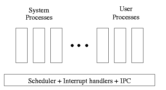
-
The above is called the client-server model and is one Tanenbaum likes.
His ``Minix'' operating system works this way.
-
Indeed, there was reason to believe that the client-server model
would dominate OS design.
But that hasn't happened.
-
Such an OS is sometimes called server based.
-
Systems like traditional unix or linux would then be
called self-service since the user process serves itself.
-
That is, the user process switches to kernel mode and performs
the system call.
-
To repeat: the same process changes back and forth from/to
user<-->system mode and services itself.
2.1.3: Implementation of Processes
The OS organizes the data about each process in a table naturally
called the process table.
Each entry in this table is called a
process table entry or PTE.
-
One entry per process.
-
The central data structure for process management.
-
A process state transition (e.g., moving from blocked to ready) is
reflected by a change in the value of one or more
fields in the PTE.
-
We have converted an active entity (process) into a data structure
(PTE). Finkel calls this the level principle ``an active
entity becomes a data structure when looked at from a lower level''.
-
The PTE contains a great deal of information about the process.
For example,
- Saved value of registers when process not running
- Stack pointer
- CPU time used
- Process id (PID)
- Process id of parent (PPID)
- User id (uid and euid)
- Group id (gid and egid)
- Pointer to text segment (memory for the program text)
- Pointer to data segment
- Pointer to stack segment
- UMASK (default permissions for new files)
- Current working directory
- Many others
An aside on Interrupts (will be done again
here)
and
here.
In a well defined location in memory (specified by the hardware) the
OS stores an interrupt vector, which contains the
address of the (first level) interrupt handler.
-
Tanenbaum calls the interrupt handler the interrupt service routine.
-
Actually one can have different priorities of interrupts and the
interrupt vector contains one pointer for each level. This is why it is
called a vector.
Assume a process P is running and a disk interrupt occurs for the
completion of a disk read previously issued by process Q, which is
currently blocked.
Note that interrupts are unlikely to be for the currently running
process (because the process waiting for the interrupt is likely
blocked).
- The hardware saves the program counter and some other registers
(or switches to using another set of registers, the exact mechanism is
machine dependent).
- Hardware loads new program counter from the interrupt vector.
- Loading the program counter causes a jump.
- Steps 1 and 2 are similar to a procedure call.
But the interrupt is asynchronous.
- As with a trap (poof), the interrupt automatically switches
the system into privileged mode.
- Assembly language routine saves registers.
- Assembly routine sets up new stack.
- These last two steps can be called setting up the C environment.
- Assembly routine calls C procedure (tanenbaum forgot this one).
- C procedure does the real work.
- Determines what caused the interrupt (in this case a disk
completed an I/O)
- How does it figure out the cause?
- Which priority interrupt was activated.
- The controller can write data in memory before the
interrupt
- The OS can read registers in the controller
- Mark process Q as ready to run.
- That is move Q to the ready list (note that again
we are viewing Q as a data structure).
- The state of Q is now ready (it was blocked before).
- The code that Q needs to run initially is likely to be OS
code. For example, Q probably needs to copy the data just
read from a kernel buffer into user space.
- Now we have at least two processes ready to run: P and Q
- The scheduler decides which process to run (P or Q or
something else). Lets assume that the decision is to run P.
- The C procedure (that did the real work in the interrupt
processing) continues and returns to the assembly code.
- Assembly language restores P's state (e.g., registers) and starts
P at the point it was when the interrupt occurred.
2.2: Interprocess Communication (IPC) and Process Coordination and
Synchronization
2.2.1: Race Conditions
A race condition occurs when two processes can
interact and the outcome depends on the order in which the processes
execute.
- Imagine two processes both accessing x, which is initially 10.
- One process is to execute x <-- x+1
- The other is to execute x <-- x-1
- When both are finished x should be 10
- But we might get 9 and might get 11!
- Show how this can happen (x <-- x+1 is not atomic)
- Tanenbaum shows how this can lead to disaster for a printer
spooler
Homework: 2
2.2.2: Critical sections
We must prevent interleaving sections of code that need to be atomic with
respect to each other. That is, the conflicting sections need
mutual exclusion. If process A is executing its
critical section, it excludes process B from executing its critical
section. Conversely if process B is executing is critical section, it
excludes process A from executing its critical section.
Requirements for a critical section implementation.
- No two processes may be simultaneously inside their critical
section.
- No assumption may be made about the speeds or the number of CPUs.
- No process outside its critical section may block other processes.
- No process should have to wait forever to enter its critical
section.
- I do NOT make this last requirement.
- I just require that the system as a whole make progress (so not
all processes are blocked).
- I refer to solutions that do not satisfy Tanenbaum's last
condition as unfair, but nonetheless correct, solutions.
- Stronger fairness conditions have also been defined.
2.2.3 Mutual exclusion with busy waiting
The operating system can choose not to preempt itself. That is, no
preemption for system processes (if the OS is client server) or for
processes running in system mode (if the OS is self service).
Forbidding preemption for system processes would prevent the problem
above where x<--x+1 not being atomic crashed the printer spooler if
the spooler is part of the OS.
But simply forbidding preemption while in system mode is not sufficient.
- Does not work for user programs. So the Unix printer spooler would
not be helped.
- Does not prevent conflicts between the main line OS and interrupt
handlers.
- This conflict could be prevented by blocking interrupts while the main
line is in its critical section.
- Indeed, blocking interrupts is often done for exactly this reason.
- Do not want to block interrupts for too long or the system
will seem unresponsive.
- Does not work if the system has several processors.
- Both main lines can conflict.
- One processor cannot block interrupts on the other.
Software solutions for two processes
Initially P1wants=P2wants=false

Code for P1                             Code for P2

Loop forever {                          Loop forever {
    P1wants <-- true         ENTRY          P2wants <-- true
    while (P2wants) {}       ENTRY          while (P1wants) {}
    critical-section                        critical-section
    P1wants <-- false        EXIT           P2wants <-- false
    non-critical-section }                  non-critical-section }
Explain why this works.
But it is wrong! Why?
================ Start Lecture #5
================
Let's try again. The trouble was that setting want before the
loop permitted us to get stuck. We had them in the wrong order!
Initially P1wants=P2wants=false

Code for P1                             Code for P2

Loop forever {                          Loop forever {
    while (P2wants) {}       ENTRY          while (P1wants) {}
    P1wants <-- true         ENTRY          P2wants <-- true
    critical-section                        critical-section
    P1wants <-- false        EXIT           P2wants <-- false
    non-critical-section }                  non-critical-section }
Explain why this works.
But it is wrong again! Why?
So let's be polite and really take turns. None of this wanting stuff.
Initially turn=1

Code for P1                      Code for P2

Loop forever {                   Loop forever {
    while (turn = 2) {}              while (turn = 1) {}
    critical-section                 critical-section
    turn <-- 2                       turn <-- 1
    non-critical-section }           non-critical-section }
This one forces alternation, so is not general enough. Specifically,
it does not satisfy condition three, which requires that no process in
its non-critical section can stop another process from entering its
critical section. With alternation, if one process is in its
non-critical section (NCS) then the other can enter the CS once but
not again.
In fact, it took years (way back when) to find a correct solution.
Many earlier ``solutions'' were found and several were published, but
all were wrong.
The first true solution was found by Dekker.
It is very clever, but I am skipping it (I cover it when I teach
masters level OS II).
Subsequently, algorithms with better fairness properties were found
(e.g., no task has to wait for another task to enter the CS twice).
What follows is Peterson's solution. When it was published, it was a
surprise to see such a simple soluntion. In fact Peterson gave a
solution for any number of processes. A proof that the algorithm
for any number of processes
satisfies our properties (including a strong fairness condition) can
be found in Operating Systems Review Jan 1990, pp. 18-22.
Initially P1wants=P2wants=false  and  turn=1

Code for P1                        Code for P2

Loop forever {                     Loop forever {
    P1wants <-- true                   P2wants <-- true
    turn <-- 2                         turn <-- 1
    while (P2wants and turn=2) {}      while (P1wants and turn=1) {}
    critical-section                   critical-section
    P1wants <-- false                  P2wants <-- false
    non-critical-section               non-critical-section
Hardware assist (test and set)
TAS(b) where b is a binary variable
ATOMICALLY sets b<--true and returns the OLD value of b.
Of course it would be silly to return the new value of b since we know
the new value is true
Now implementing a critical section for any number of processes is trivial.
loop forever {
    while (TAS(s)) {}   ENTRY
    CS
    s<--false           EXIT
    NCS
P and V and Semaphores
Note: Tanenbaum does both busy waiting (like above)
and blocking (process switching) solutions. We will only do busy
waiting.
Homework: 3
The entry code is often called P and the exit code V (Tanenbaum only
uses P and V for blocking, but we use it for busy waiting). So the
critical section problem is to write P and V so that
loop forever
    P
    critical-section
    V
    non-critical-section
satisfies
- Mutual exclusion
- No speed assumptions
- No blocking by processes in NCS
- Forward progress (my weakened version of Tanenbaum's last condition
Note that I use indenting carefully and hence do not need (and
sometimes omit) the braces {}
A binary semaphore abstracts the TAS solution we gave
for the critical section problem.
The above code is not real, i.e., it is not an
implementation of P. It is, instead, a definition of the effect P is
to have.
To repeat: for any number of processes, the critical section problem can be
solved by
loop forever
    P(S)
    CS
    V(S)
    NCS
The only specific solution we have seen for an arbitrary number of
processes is the one just above with P(S) implemented via
test and set.
Remark: Peterson's solution requires each process to
know its processor number. The TAS soluton does not.
Moreover the definition of P and V does not permit use of the
processor number.
Thus, strictly speaking Peterson did not provide an implementation of
P and V.
He did solve the critical section problem.
To solve other coordination problems we want to extend binary
semaphores.
- With binary semaphores, two consecutive Vs do not permit two
subsequent Ps to succeed (the gate cannot be doubly opened).
- We might want to limit the number of processes in the section to
3 or 4, not always just 1.
The solution to both of these shortcomings is to remove the
restriction to a binary variable and define a
generalized or counting semaphore.
- A counting semaphore S takes on non-negative integer values
- Two operations are supported
- P(S) is
    while (S=0)
    S--
where finding S>0 and decrementing S is atomic
- That is, wait until the gate is open (positive), then run through and
atomically close the gate one unit
- Said another way, it is not possible for two processes doing P(S)
simultaneously to both see the same positive value of S unless a V(S)
is also simultaneous.
- V(S) is simply S++
These counting semaphores can solve what I call the
semi-critical-section problem, where you premit up to k
processes in the section. When k=1 we have the original
critical-section problem.
initially S=k

loop forever
    P(S)
    SCS   <== semi-critical-section
    V(S)
    NCS
================ Start Lecture #6
================
Producer-consumer problem
- Two classes of processes
- Producers, which produce times and insert them into a buffer.
- Consumers, which remove items and consume them.
- What if the producer encounters a full buffer?
Answer: Block it.
- What if the consumer encounters an empty buffer?
Answer: Block it.
- Also called the bounded buffer problem.
- Another example of active entities being replaced by a data
structure when viewed at a lower level (Finkel's level principle).
Initially e=k, f=0 (counting semaphore); b=open (binary semaphore)

Producer                         Consumer

loop forever                     loop forever
    produce-item                     P(f)
    P(e)                             P(b); take item from buf; V(b)
    P(b); add item to buf; V(b)      V(e)
    V(f)                             consume-item
- k is the size of the buffer
- e represents the number of empty buffer slots
- f represents the number of full buffer slots
- We assume the buffer itself is only serially accessible. That is,
only one operation at a time.
- This explains the P(b) V(b) around buffer operations
- I use ; and put three statements on one line to suggest that
a buffer insertion or removal is viewed as one atomic operation.
- Of course this writing style is only a convention, the
enforcement of atomicity is done by the P/V.
- The P(e), V(f) motif is used to force ``bounded alternation''. If k=1
it gives strict alternation.
Dining Philosophers
A classical problem from Dijkstra
- 5 philosophers sitting at a round table
- Each has a plate of spaghetti
- There is a fork between each two
- Need two forks to eat
What algorithm do you use for access to the shared resource (the
forks)?
- The obvious solution (pick up right; pick up left) deadlocks.
- Big lock around everything serializes.
- Good code in the book.
The purpose of mentioning the Dining Philosophers problem without giving
the solution is to give a feel of what coordination problems are like.
The book gives others as well. We are skipping these (again this
material would be covered in a sequel course). If you are interested
look, for example,
here.
Homework: 14,15 (these have short answers but are
not easy).
Readers and writers
- Two classes of processes.
- Readers, which can work concurrently.
- Writers, which need exclusive access.
- Must prevent 2 writers from being concurrent.
- Must prevent a reader and a writer from being concurrent.
- Must permit readers to be concurrent when no writer is active.
- Perhaps want fairness (i.e., freedom from starvation).
- Variants
- Writer-priority readers/writers.
- Reader-priority readers/writers.
Quite useful in multiprocessor operating systems. The ``easy way
out'' is to treat all processes as writers in which case the problem
reduces to mutual exclusion (P and V). The disadvantage of the easy
way out is that you give up reader concurrency.
Again for more information see the web page referenced above.
================ Start Lecture #7
================
2.4: Process Scheduling
Scheduling the processor is often called ``process scheduling'' or simply
``scheduling''.
The objectives of a good scheduling policy include
- Fairness.
- Efficiency.
- Low response time (important for interactive jobs).
- Low turnaround time (important for batch jobs).
- High throughput [the above are from Tanenbaum].
- Repeatability. Dartmouth (DTSS) ``wasted cycles'' and limited
logins for repeatability.
- Fair across projects.
- ``Cheating'' in unix by using multiple processes.
- TOPS-10.
- Fair share research project.
- Degrade gracefully under load.
Recall the basic diagram describing process states
For now we are discussing short-term scheduling, i.e., the arcs
connecting running <--> ready.
Medium term scheduling is discussed later.
Preemption
It is important to distinguish preemptive from non-preemptive
scheduling algorithms.
- Preemption means the operating system moves a process from running
to ready without the process requesting it.
- Without preemption, the system implements ``run to completion (or
yield or block)''.
- The ``preempt'' arc in the diagram.
- We do not consider yield (a solid arrow from running to ready).
- Preemption needs a clock interrupt (or equivalent).
- Preemption is needed to guarantee fairness.
- Found in all modern general purpose operating systems.
- Even non preemptive systems can be multiprogrammed (e.g., when processes
block for I/O).
Deadline scheduling
This is used for real time systems. The objective of the scheduler is
to find a schedule for all the tasks (there are a fixed set of tasks)
so that each meets its deadline. The run time of each task is known
in advance.
Actually it is more complicated.
- Periodic tasks
- What if we can't schedule all task so that each meets its deadline
(i.e., what should be the penalty function)?
- What if the run-time is not constant but has a known probability
distribution?
We do not cover deadline scheduling in this course.
The name game
There is an amazing inconsistency in naming the different
(short-term) scheduling algorithms. Over the years I have used
primarily 4 books: In chronological order they are Finkel, Deitel,
Silberschatz, and Tanenbaum. The table just below illustrates the
name game for these four books. After the table we discuss each
scheduling policy in turn.
Finkel  Deitel  Silbershatz Tanenbaum
-------------------------------------
FCFS    FIFO    FCFS        --    unnamed in tanenbaum
RR      RR      RR          RR
PS      **      PS          PS
SRR     **      SRR         **    not in tanenbaum
SPN     SJF     SJF         SJF
PSPN    SRT     PSJF/SRTF   --    unnamed in tanenbaum
HPRN    HRN     **          **    not in tanenbaum
**      **      MLQ         **    only in silbershatz
FB      MLFQ    MLFQ        MQ
First Come First Served (FCFS, FIFO, FCFS, --)
If the OS ``doesn't'' schedule, it still needs to store the PTEs
somewhere. If it is a queue you get FCFS. If it is a stack
(strange), you get LCFS. Perhaps you could get some sort of random
policy as well.
- Only FCFS is considered.
- The simplist scheduling policy.
- Non-preemptive.
Round Robbin (RR, RR, RR, RR)
- An important preemptive policy.
- Essentially the preemptive version of FCFS.
- The key parameter is the quantum size q.
- When a process is put into the running state a timer is set to q.
- If the timer goes off and the process is still running, the OS
preempts the process.
- This process is moved to the ready state (the
preempt arc in the diagram), where it is placed at the
rear of the ready list (a queue).
- The process at the front of the ready list is removed from
the ready list and run (i.e., moves to state running).
- When a process is created, it is placed at the rear of the ready list.
- As q gets large, RR approaches FCFS
- As q gets small, RR approaches PS (Processor Sharing, described next)
- What value of q should we choose?
- Tradeoff
- Small q makes system more responsive.
- Large q makes system more efficient since less process switching.
Homework: 9, 19, 20, 21, and the following (remind
me to discuss this last one in class next time):
Consider the set of processes in the table below.
When does each process finish if RR scheduling is used with q=1, if
q=2, if q=3, if q=100. First assume (unrealistically) that context
switch time is zero. Then assume it is .1.
Each process performs no
I/O (i.e., no process ever blocks). All times are in milliseconds.
The CPU time is the total time required for the process (excluding
context switch time). The creation
time is the time when the process is created. So P1 is created when
the problem begins and P2 is created 5 miliseconds later.
| Process | CPU Time | Creation Time |
|---|
| P1 | 20 | 0 |
| P2 | 3 | 3 |
| P3 | 2 | 5 |
Processor Sharing (PS, **, PS, PS)
Merge the ready and running states and permit all ready jobs to be run
at once. However, the processor slows down so that when n jobs are
running at once each progresses at a speed 1/n as fast as it would if
it were running alone.
- Clearly impossible as stated due to the overhead of process
switching.
- Of theoretical interest (easy to analyze).
- Approximated by RR when the quantum is small. Make
sure you understand this last point. For example,
consider the last homework assignment (with zero context switch time)
and consider q=1, q=.1, q=.01, etc.
Homework: 18. (part of homework #8 as #7 has enough)
Variants of Round Robbin
- State dependent RR
- Same as RR but q is varied dynamically depending on the state
of the system.
- Favor processes holding important resources.
- For example, non-swappable memory.
- Perhaps this should be considered medium term scheduling
since you probably do not recalculate q each time.
- External priorities: RR but a user can pay more and get
bigger q. That is one process can be given a higher priority than
another. But this is not an absolute priority, i.e., the lower priority
(i.e., less important) process does get to run, but not as much as the
high priority process.
Priority Scheduling
Each job is assigned a priority (externally, perhaps by charging
more for higher priority) and the highest priority ready job is run.
- Similar to ``External priorities'' above
- If many processes have the highest priority, use RR among them.
- Can easily starve processes (see aging below for fix).
- Can have the priorities changed dynamically to favor processes
holding important resources (similar to state dependent RR).
- Many policies can be thought of as priority scheduling in
which we run the job with the highest priority (with different notions
of priority for different policies).
Priority aging
As a job is waiting, raise its priority so eventually it will have the
maximum priority.
- This prevents starvation (assuming all jobs terminate).
policy is preemptive).
- There may be many processes with the maximum priority.
- If so, can use fifo among those with max priority (risks
starvation if a job doesn't terminate) or can use RR.
- Can apply priority aging to many policies, in particular to priority
scheduling described above.
================ Start Lecture #8
================
Homework: 22, 23
Selfish RR (SRR, **, SRR, **)
- Preemptive.
- Perhaps it should be called ``snobbish RR''.
- ``Accepted processes'' run RR.
- Accepted process have their priority increase at rate b>=0.
- A new process starts at priority 0; its priority increases at rate a>=0.
- A new process becomes an accepted process when its priority
reaches that of an accepted process (or until there are no accepted
processes).
- Note that at any time all accepted processes have same priority.
- If b>=a, get FCFS.
- If b=0, get RR.
- If a>b>0, it is interesting.
Shortest Job First (SPN, SJF, SJF, SJF)
Sort jobs by total execution time needed and run the shortest first.
- Nonpreemptive
- First consider a static situation where all jobs are available in
the beginning, we know how long each one takes to run, and we
implement ``run-to-completion'' (i.e., we don't even switch to another
process on I/O). In this situation, SJF has the shortest average
waiting time
- Assume you have a schedule with a long job right before a
short job.
- Consider swapping the two jobs.
- This decreases the wait for
the short by the length of the long job and increases the wait of the
long job by the length of the short job.
- This decreases the total waiting time for these two.
- Hence decreases the total waiting for all jobs and hence decreases
the average waiting time as well.
- Hence, whenever a long job is right before a short job, we can
swap them and decrease the average waiting time.
- Thus the lowest average waiting time occurs when there are no
short jobs right before long jobs.
- This is SJF.
- In the more realistic case where the scheduler switches to a new
process when the currently running process blocks (say for I/O), we
should call the policy shortest next-CPU-burst first.
- The difficulty is predicting the future (i.e., knowing in advance
the time required for the job or next-CPU-burst).
- This is an example of priority scheduling.
Preemptive Shortest Job First (PSPN, SRT, PSJF/SRTF, --)
Preemptive version of above
- Permit a process that enters the ready list to preempt the running
process if the time for the new process (or for its next burst) is
less than the remaining time for the running process (or for
its current burst).
- It will never happen that a process in the ready list
will require less time than the remaining time for the currently
running process. Why?
Ans: When the process joined the ready list it would have started
running if the current process had more time remaining. Since
that didn't happen the current job had less time remaining and now
it has even less.
- Can starve processs that require a long burst.
- This is fixed by the standard technique.
- What is that technique?
Ans: Priority aging.
- Another example of priority scheduling.
Highest Penalty Ratio Next (HPRN, HRN, **, **)
Run the process that has been ``hurt'' the most.
- For each process, let r = T/t; where T is the wall clock time this
process has been in system and t is the running time of the process to
date.
- If r=5, that means the job has been running 1/5 of the time it has been
in the system.
- We call r the penalty ratio and run the process having
the highest r value.
- HPRN is normally defined to be non-preemptive (i.e., the system
only checks r when a burst ends), but there is an preemptive analogue
- Do not worry about a process that just enters the system (its
ratio is undefined)
- When putting process into the run state commpute the time at
which it will no longer have the highest ratio and set a timer.
- When a process is moved into the ready state, compute its ratio
and preempt if needed.
- HRN stands for highest response ratio next and means the same thing.
- This policy is another example of priority scheduling
Multilevel Queues (**, **, MLQ, **)
Put different classes of processs in different queues
- Processs do not move from one queue to another.
- Can have different policies on the different queues.
For example, might have a background (batch) queue that is FCFS and one or
more foreground queues that are RR.
- Must also have a policy among the queues.
For example, might have two queues, foreground and background, and give
the first absolute priority over the second
- Might apply aging to prevent background starvation.
- But might not, i.e., no guarantee of service for background
processes. View a background process as a ``cycle soaker''.
- Might have 3 queues, foreground, background, cycle soaker
Multilevel Feedback Queues (FB, MFQ, MLFBQ, MQ)
Many queues and processs move from queue to queue in an attempt to
dynamically separate ``batch-like'' from interactive processs.
- Run processs from the highest priority nonempty queue in a RR manner.
- When a process uses its full quanta (looks a like batch process),
move it to a lower priority queue.
- When a process doesn't use a full quanta (looks like an interactive
process), move it to a higher priority queue.
- A long process with frequent (perhaps spurious) I/O will remain
in the upper queues.
- Might have the bottom queue FCFS.
- Many variants
For example, might let process stay in top queue 1 quantum, next queue 2
quanta, next queue 4 quanta (i.e. return a process to the rear of the
same queue it was in if the quantum expires).
Theoretical Issues
Considerable theory has been developed.
- NP completeness results abound.
- Much work in queuing theory to predict performance.
- Not covered in this course.
Medium Term scheduling
Decisions made at a coarser time scale.
- Called two-level scheduling by Tanenbaum.
- Suspend (swap out) some process if memory is over-committed.
- Criteria for choosing a victim.
- How long since previously suspended.
- How much CPU time used recently.
- How much memory does it use.
- External priority (pay more, get swapped out less).
- We will discuss medium term scheduling again next chapter (memory
management).
Long Term Scheduling
- ``Job scheduling''. Decide when to start jobs, i.e., do not
necessarily start them when submitted.
- Force user to log out and/or block logins if over-committed.
- CTSS (an early time sharing system at MIT) did this to insure
decent interactive response time.
- Unix does this if out of processes (i.e., out of PTEs)
- ``LEM jobs during the day'' (Grumman).
- Some supercomputer sites.
================ Start Lecture #9
================
Notes on lab (scheduling)
- If several processes are waiting on I/O, you may assume
noninterference. For example, assume that on cycle 100 process A
flips a coin and decides its wait is 6 units (i.e., during cycles
101-106 A will be blocked. Assume B begins running at cycle 101 for a
burst of 1 cycle. So during 101
process B flips a coin and decides its wait is 3 units. You do NOT
have to alter process A. That is, Process A will become ready after
cycle 106 (100+6) so enters the ready list cycle 107 and process B
becomes ready after cycle 104 (101+3) and enters ready list cycle
105.
- For processor sharing (PS), which is part of the extra credit:
PS (processor sharing). Every cycle you see how many jobs are
in the ready Q. Say there are 7. Then during this cycle (an exception
will be described below) each process gets 1/7 of a cycle.
EXCEPTION: Assume there are exactly 2 jobs in RQ, one needs 1/3 cycle
and one needs 1/2 cycle. The process needing only 1/3 gets only 1/3,
i.e. it is finished after 2/3 cycle. So the other process gets 1/3
cycle during the first 2/3 cycle and then starts to get all the CPU.
Hence it finishes after 2/3 + 1/6 = 5/6 cycle. The last 1/6 cycle is
not used by any process.
Allan Gottlieb