Applying the Constellation Model to Google Data

Preliminaries

The Constellation Model is a sparse, parts and structure type model. If you are not familiar with it, please read here.

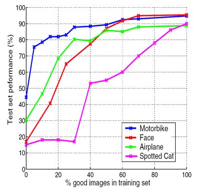
How will such a model fare when learning from Google data? The results of a preliminary experiment, shown in the plot below, give some encouragement. The experiment involved the training and testing of a standard Constellation Model on four manually gathered datasets (Caltech 4). On the x-axis we vary the portion of unrelated images in training set with the test performance of the learnt model plotted on the y-axis. As the portion of good images drops, the performance of the models does not degrade significantly (except for the spotted cats) until below 20-30%. As seen on the previous page, this is around the level of contamination in the data returned by Google's Image Search, so there is some chance that this model may work effectively.

Adaptations to Google Data

The original set of features used by the Constellation Model consisted of one type of feature detector that finds textured regions. Given the variability of the data returned by Google and the importance of providing the model with informative features, we augment the model with additional feature types. In addition to the Kadir & Brady interest operator [1] (the output of which is shown on the example on the left below), we employ a curve feature to capture the outlines of objects rather than their textured interior (center) and a multi-scale Harris operator [2] (right).

.

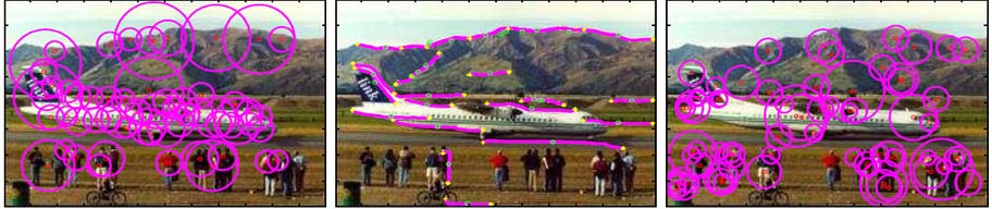For each query, a set of models, each using 6 parts but with a different combination of feature types is trained. The combination that performs best on the automatically acquired validation set is chosen as the winning model that will be used in testing.

Some Examples of Models Trained from Google Data

Below is a model trained from images returned by the query "wrist watch" in Google. On the left is an example image, with the feature detections overlaid as magenta dots (indicating center of region) and curves. On the right are the regions closest to the mean of each appearance distribution of each part. The K and C symbols indicate if the part is a Kadir and Brady region (K), a curve feature (C) or a multi-scale Harris (H). The appearance samples are noisy, but the model would seem to have captured the curved bezel structure of the watch.

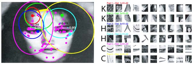
The next image shows a model trained from the query "faces". The model has a very large variance and it is not clear exactly what features it is using, but it is possibly the hairline on the face.

It is apparent that both models have a very high variance in their spatial layout and would appear to be rather weak. On the main page, we compare these models with our bag-of-words type model.

References

[1] Scale, Saliency and Image Description. T. Kadir and M. Brady. International Journal of Computer Vision, 45(2):83-105, 2001.

[2] Indexing Based on Scale Invariant Interest Points. K. Mikolajczyk and C. Schmid. Proceedings of the 8th International Conference on Computer Vision, Vancouver, Canada, pages 525-531, 2001.