Algorithms

Our goal is to choose one tree from each gene, then combine those trees into a direct acyclic graph with the fewest interbreeding events. The algorithm can be described in two stages: tree selecting and tree combining. 

Our goal is to select one tree from each gene. Therefore we would like to select popular trees since they immediately "cover" may genes. If there is a single tree suggested by all genes, then it suffices to select only that tree. But usually we will see the following situation:

gene g1 suggests trees t1, t3, t5
gene g2 suggests trees t1, t2, t4
gene g3 suggests trees t1, t6, t4
gene g4 suggests trees t1, t6, t5
gene g5 suggests trees t2, t4, t7
gene g6 suggests trees t3, t5, t8

In this example we can select trees {t1,t2,t3} to cover all genes (at least one tree from each gene). These kind of problems are called hitting set problems. The fewer trees we select, the easier to combine them with a few interbreeding events (This statement is questionable since it would be harder to combine two totally different trees than to combine many similar trees. In practice, however, it turns out that popular trees usually share some common structures and will be similar after all). Therefore we would like to pick the smallest hitting set. So in the above example, {t4,t5} will be the right choice. Such problem is called minimum hitting set problem. In this software, we have developed a hitting set solver to solve it efficiently. See algorithms of the hitting set solver for more details.

Another thing we might want to do is to ignore trees that rarely appear in the input data since they are supported by very few evidence. Therefore we set a cutoff frequency F in the software to discard trees that appear less than F times in the data. If some genes are so eccentric such that every trees they suggest are discarded, then we ignore these genes as well. The developed algorithm is called Consensus Method:

1. U <-- the set of all gene trees (duplicates removed)
2. U <-- U - {t | tree t appear less than F times in the input}
3. S <-- empty set
4. for each gene g do
5.     R <-- {t | t belongs to U and is suggested by g}
6.     Append R to S
7. for i in [1..MAX_ITERATION] do
8.     C_i <-- Hitting_Set_Solver(S, U)
9. return tree collection C_x which requires the fewest interbreeding events to be combined

The results can be found in the software webpage.

Consensus method selects trees based on their popularity. However, if all trees appear only once (or very few times) in the data, it is much meaningless to use this method. That is, in that case it works better to select similar trees from each gene instead of looking for identical trees. For this purpose we first define the similarity between trees:

Definition:

1. The distance between two trees:
   distance(T₁, T₂) = the smallest number of interbreeding events needed to combine T₁ and T₂.
2. Similarity: two trees are said to be similar if the distance between them is small.

Once we define the similarity, we can easily come up with some greedy algorithms for tree selecting:

• Similar to first heuristics:
  
  1. Pick an arbitrary tree T₁ from the first gene
  2. for the i^th gene do
  3.     Pick the tree T_i such that distance(T₁, T_i) is minimized
  4. return {T₁, T₂, ...}
• Similar to last heuristics:
  
  1. Pick an arbitrary tree T₁ from the first gene
  2. for the i^th gene do
  3.     Pick the tree T_i such that distance(T_i-1, T_i) is minimized
  4. return {T₁, T₂, ...}

• Randomized hybrid heuristics:
  
  1. Pick an arbitrary tree T₁ from arbitrary gene
  2. for each other gene (in a random order) do
  3.     Pick the tree T_i such that distance(T₁, T_i) + distance(T_i-1, T_i) is minimized
  4. return {T₁, T₂, ...}

Definitions:

• Evaluation of a tree collection:
  Let C be a collection of gene trees (one tree from each gene).
  Evaluation(C) = (The smallest number of interbreeding events needed to combine C into a graph) *K + (Total score/rank of trees in C)
  Here K is a large enough constant such that the first term will dominate the function (Remember the scores of trees are merely used for tie-breaking). A tree collection is better if the evaluation score is smaller.
• Neighbor of a tree collection:
  Let C be a collection of gene trees (one tree from each gene). A neighbor C' of C is obtained by the following random process: for each gene with probability 1-p we include the corresponding gene tree in C to C'. Otherwise (with probability p) randomly pick a gene tree from that gene and add it to C'. In our software p was set to the inverse of the number of genes. Therefore the expected number of changes from C to C' will be 1.

Algorithm:

Simulated_Annealing(T₀, T, alpha):
1. Pick a starting collection C using randomized hybrid heuristics
2. t <-- T₀
3. while t > T do
4.     Choose a neighbor C' of C
5.     d <-- Evaluation(C) - Evaluation(C')
6.     if d > 0 then
7.         C <-- C'
8.     else with probability e^d/t :
9.         C <-- C'
10.     t <-- t * alpha
11. return the best tree collection seen through the whole process

Here T₀ and T stands for initial and final temperature, respectively, while the temperature decreases exponentially with a factor alpha every iteration. Note that even if the neighbor is worse than the current solution, there is still some chance for the algorithm to switch to it (especially when t is large since the probability of switching = e^d/t). That means it is possible to get out of local minimum, which is an important feature. The spirit of this algorithm is that the initial high temperature will make the whole system unstable. Then the temperature cools down slowly, making it harder to switch without benefit. See an introduction to simulated annealing for more insight.

In this problem, a single bad tree could poison the solution seriously. So in actual experiments the original greedy solution was rarely improved much. Therefore instead of running a long annealing process, we also might want to restart the algorithm several times to explore the search space as much as we can. This is the final algorithm we developed. The experimental results can be found in the software webpage.

We use the following example (Trees are given in the Newick tree format):

geneA: ((s1 (s2 s3) s4 s5) (s6 s7 s8))
geneB: ((s6 (s1 s2) s7 (s3 s4)) (s5 s8))

Orthologs:
s1: {geneA_11, geneB_121}
s2: {geneA_121, geneB_122}
s3: {geneA_122, geneB_141}
s4: {geneA_13, geneB_142}
s5: {geneA_14, geneB_21}
s6: {geneA_21, geneB_11}
s7: {geneA_22, geneB_13}
s8: {geneA_23, geneB_22}

All trees here are unordered, that is, the order of siblings is unimportant. So the Newick tree representation is not unique. For example, the following two trees are equivalent to the above two:

geneA: ((s6 s7 s8) (s1 (s2 s3) s4 s5))
geneB: ((s6 s7 (s1 s2) (s3 s4)) (s5 s8))

Also, in Newick tree format, a pair of parentheses corresponds to an internal node of the tree which is the nearest common ancestor for all species enclosed by that parentheses. For a better illustration, see our introduction.

Definitions:

• Group:
  A subset of species S forms a group if each gene tree has a Newick tree representation such that we can insert a pair of parentheses into that representation to enclose only species in S without destroying the well-parenthesized structure in every tree.
• Minimal Group:
  A group which contains no smaller group. Note that if A and B are both groups, then the intersection of them will also be a group. Therefore for any two groups A and B, one of the following relationship holds: (1) A and B are disjoint. (2) A is a subset of B. (3) B is a subset of A. This proposition ensures the existence of the minimal group.
• Relationship:
  
  • Species A and B have a closer relationship than do A and C if the nearest common ancestor of A and B is a descendent of the nearest common ancestor of A and C.
  • In parentheses representation, A and B have a closer relationship than do A and C if the innermost parentheses enclosing both A and B does not enclose C.
  • In subscript representation, A and B have a closer relationship than do A and C if the longest common prefix of the subscripts of A and B is longer than is the longest common prefix of subscripts of A and C.

Example:

• In the above example, a pair of parentheses can be inserted in the first tree to enclose [s1 s2 s3] but not in the second tree. So [s1 s2 s3] is not a group. In fact, there are only three groups:
  1. [s1 s2 s3 s4]
  2. [s6 s7]
  3. [s1 s2 s3 s4 s5 s6 s7 s8]
  The third one is the trivial group which contains all species. Group [s1 s2 s3 s4] and [s6 s7] are both minimal while the trivial group is not.
• In the first tree, s3 and s5 have a closer relationship than s3 and s7. In the second tree, however, they have a farther relationship than s3 and s7.

Theorem:

1. If s1 and s3 have a closer relationship than do s1 and s2 in some gene tree, then any group containing both s1 and s2 must also contains s3.
2. Assume G is the optimum combined graph, i.e., the one with the fewest interbreeding events. If a subset of species S forms a group, then G has a subtree T whose leaf set is exactly S. The root of T is the common ancestor of species in S. In other words, the descendant set of the root of T is S.
3. Let S be the descendant set of species A. In that case, the subscripts of orthologs in A will be the longest common prefixes of all corresponding orthologs in species of S.

Therefore, the algorithm can be described as the following:

Main algorithm

1. Grouping: Find all groups in the input data.
2. Find a minimal group whose species set is denoted by S.
3. For every gene tree extract the subtree containing only S. Combine these subtrees into a small graph G with the fewest interbreeding events.
4. In the original trees, replace S by their common ancestor which is the root of G.
5. Insert G to our final graph.
6. Repeat step 2~5 till there is only one species left. That species will be the root of the final graph.

Example:

• Assume our program chooses [s1 s2 s3 s4] as the first minimal group to process, the corresponding subtrees will be:
  (s1 (s2 s3) s4)
  ((s1 s2) (s3 s4)) -- Combining Problem 1
  The next step is to combine these two trees and replace [s1 s2 s3 s4] by a hypothetical extinct ancestral species miss1 in original trees:
  geneA: ((s1 (s2 s3) s4 s5) (s6 s7 s8))   --> ((miss1 s5) (s6 s7 s8))
  geneB: ((s6 (s1 s2) s7 (s3 s4)) (s5 s8)) --> ((s6 miss1 s7) (s5 s8))
  miss1 contains orthologs {geneA_1, geneB_1}
• The next minimal group will be [s6 s7]. The corresponding subtrees:
  (s6 s7)
  (s6 s7) -- Combining Problem 2
  Replace [s6 s7] by a hypothetical extinct ancestral species miss2 in original trees:
  geneA: ((miss1 s5) (s6 s7 s8)) --> ((miss1 s5) (miss2 s8))
  geneB: ((s6 miss1 s7) (s5 s8)) --> ((miss2 miss1) (s5 s8))
  miss2 contains orthologs {geneA_2, geneB_1}
• Now only the trivial group [s5 s8 miss1 miss2] is left and we get the final subtree combining problem:
  ((miss1 s5) (miss2 s8))
  ((miss2 miss1) (s5 s8)) -- Combining Problem 3
  Replace [s5 s8 miss1 miss2] by a hypothetical extinct ancestral species miss3 in original trees:
  geneA: ((miss1 s5) (miss2 s8)) --> miss3
  geneB: ((miss2 miss1) (s5 s8)) --> miss3
  miss3 contains orthologs {geneA_, geneB_}
• miss3 will be the root of the combined graph.

Next step will be solving the tree combining problems in the previous stage. The basic strategy is to remove a minimum number of problematic species that cause conflicts, and then combine all gene trees into one big tree (That is, after removing those species all trees become mutually consistent). After that, insert some intermediate missing species to complete the gene deriving steps. Finally, pair up the removed species with proper parents and transform the big tree into a graph.

Definitions:

• Conflict Triples:  species A, B and C form a conflict triple if A and B have a closer relationship than do A and C in gene tree T₁, but have a farther relationship than do A and C in tree T₂

Theorem:

Several trees can be combined into a big tree if and only if there is no conflict triple.

Example:

• 2 conflict triples (s1,s2,s3) and (s2,s3,s4) in combining problem 1:
  (s1 (s2 s3) s4)
  ((s1 s2) (s3 s4))
  
• 0 conflict triples in combining problem 2:
  (s6 s7)
  (s6 s7)
  
• 4 conflict triples (miss1,miss2,s5), (miss1,miss2,s8), (miss1,s5,s8) and (miss2,s5,s8) in combining problem 3:
  ((miss1 s5) (miss2 s8))
  ((miss2 miss1) (s5 s8))
  

Therefore our approach can be described as the following:

1. Choose a minimal set of species S and remove them such that there is no conflict triple left
2. Combine all trees into one tree
3. Insert the removed species back with proper parents

Here we assume the species removed came from interbreeding events. So at the last step we will actually associate each of them with multiple parents.

Clearly, if at the beginning we have a conflict triple (A,B,C), either A or B or C must be in S, otherwise the removal of S will not eliminate this triple. So again we get a hitting set problem:

Definition:

• Hitting set: Let C be a collection of sets. H is a hitting set of C if the intersection of H and any set in C is non-empty.
• A hitting set is minimal if the removal of any element will destroy the hitting set. A hitting set is minimum if it has the smallest size over all hitting sets.
• Minimum hitting set problem H(C,K): C is a collection of subsets of K. Find the minimum hitting set H of C. In this case H will always be a subset of K.

Example:

• Let K = {1,2,3,4,5,6,7}, C = {{1,4,5}, {1,2,3}, {2,6,7}, {1,3,7}}. {3,4,6} will be a minimal hitting set (yet not minimum). In this example, {1,2}, {1,6} and {1,7} are the only minimum hitting sets.
• In combining problem 1, the minimum hitting set of { (s1,s2,s3), (s2,s3,s4)} is either {s2} or {s3}.
• In combining problem 3, the minimum hitting set of { (miss1,miss2,s5), (miss1,miss2,s8), (miss1,s5,s8), (miss2,s5,s8)} has size 2. In fact, any size 2 subset is a minimum hitting set.

We can model each conflict triple as a set of size 3 and K the set of all species. Then the species removing problem in step 1 becomes a hitting set problem. A hitting set solver was developed to solve this NP-complete problem (The hitting set problem remains NP-complete even under the constraint that every set has size 3). Once we find the hitting set, we remove those species from all trees. Now we should be able to combine the rest into a big tree (See Theorem above). In fact this can be done by the same steps in the main algorithm (See the following example).

Example:

• Assume we picked {s2} as the minimum hitting set and removed it from the combining problem 1:
  geneA: (s1 (s2 s3) s4)   --> (s1 (s3) s4)
  geneB: ((s1 s2) (s3 s4)) --> ((s1) (s3 s4))
  
• Now the [s3 s4] is a minimal group. Replace it by a hypothetical species miss4 :
  geneA: (s1 (s3) s4)   --> (s1 miss4)
  geneB: ((s1) (s3 s4)) --> ((s1) miss4)
  miss4 contains orthologs {geneA_1, geneB_14}
• Then only the trivial group [s1 miss4] is left and we replace it by species miss5 :
  geneA: (s1 miss4)  --> miss5
  geneB: ((s1) miss4)--> miss5
  miss5 contains orthologs {geneA_1, geneB_1}

• miss5 will be the root of the subgraph. Note that miss1 mentioned above has the same ortholog set with miss5, so they are actually the same species. Let's use miss1 to represent the root. The combined subgraph:

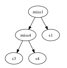
After combining the subtrees, we complete gene deriving steps by inserting intermediate hypothetical species.

Example:

• From above we inferred that miss4 {geneA_1, geneB_14} is an ancestor of s3 {geneA_122, geneB_141}. But there are 3 gene mutation steps happening in between: geneA_1 --> geneA_12, geneA_12 --> geneA_122 and geneB_14 --> geneB_141. Therefore there are 3 possible evolutionary path:
  1. {geneA_1, geneB_14} --> {geneA_12, geneB_14} --> {geneA_122, geneB_14} --> {geneA_122, geneB_141}
  2. {geneA_1, geneB_14} --> {geneA_12, geneB_14} --> {geneA_12, geneB_141} --> {geneA_122, geneB_141}
  3. {geneA_1, geneB_14} --> {geneA_1, geneB_141} --> {geneA_12, geneB_141} --> {geneA_122, geneB_141}
• Deciding which path yields fewer interbreeding events in the final graph is an NP-hard problem. Therefore our software will randomly choose one path. Say we take the first one, the intermediate species inserted will be miss6 {geneA_12, geneB_14} and miss7 {geneA_122, geneB_14}. Similarly, assume we insert the following paths (edges) to this graph:
  • miss4 {geneA_1, geneB_14} --> miss6 {geneA_12, geneB_14} --> miss7 {geneA_122, geneB_14} --> s3 {geneA_122, geneB_141}
  • miss4 {geneA_1, geneB_14} --> miss8 {geneA_13, geneB_14} --> s4 {geneA_13, geneB_142}
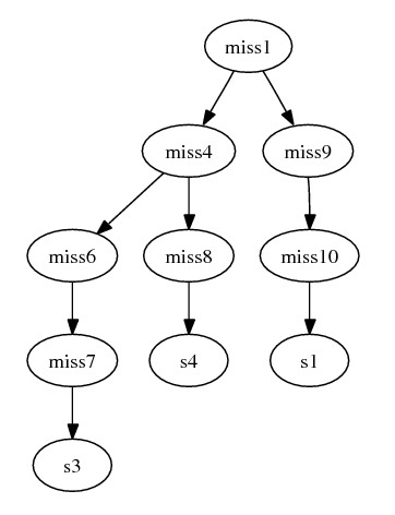
  • miss1 {geneA_1, geneB_1} --> miss9 {geneA_11, geneB_14} --> miss10 {geneA_11, geneB_12} --> s1 {geneA_11, geneB_121}
  • miss1 {geneA_1, geneB_1} --> miss4 {geneA_1, geneB_14}
• The combined graph becomes:

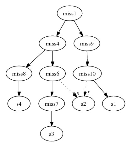
Finally, we infer the parents of removed species by their orthologs.

Example:

• Here is only one removed species: s2 {geneA_121, geneB_122}. Recall that geneA_121 must be derived from geneA_12 and miss6 is the only species containing that ortholog in this subgraph. Therefore miss6 must be a parent of s2. Similarly, since miss10 is the only species containing ortholog geneB_12 for deriving geneB_122, it must also be a parent of s2. The final subgraph:

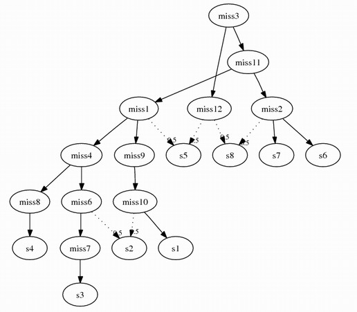
Following this algorithm, assume we remove s5 and s8 from combining problem 3, 2 more intermediate species will be inserted:

miss11 {geneA_, geneB_1}
miss12 {geneA_, geneB_2}

The complete combined graph:

We start with a set of two species and recursively bring in species which are close to some species in the set. The algorithm can be described as the following:

1. Arbitrarily pick species s1 and s2
2. s⁺ <-- {s1, s2}
3. Until s⁺ does not change do
4.     Consider a species t outside s⁺ :
5.     for each gene g and any two species x, y in s⁺ :
6.         if x and t have a closer relationship than do y and t then
7.             Add t into s⁺
8.             break
9. return s⁺

Repeat this procedure with all possible combinations of s1 and s2 such that we can obtain all possible groups (There are some minor things to be worried about. For more details, see the paper).

Here we introduce three approximation/heuristic algorithms solving the general hitting set problem.

1. H <-- empty set
2. while H not yet hit all set in C do
3.     Pick a set not yet hit, add every element in that set to H
4. return H

Note in our case that every set in C has size 3, this algorithm has a theoretical guarantee: if the minimum hitting set has size k, then the size of the returned hitting set will not exceed 3k. In computer science jargon, we say this algorithm yields an approximation factor of 3. However, practically it doesn't work very will. This algorithm might not even report a minimal hitting set! For the above example, the output would be {1,4,5,2,6,7} whose size is exactly 3 times the optimum size. In our program, redundant elements in the solution are removed such that the final output will be minimal. However, the performance is still not that great in general. We kept this implementation merely because it reaches the best known approximation ratio.

1. H <-- empty set
2. while H not yet hit all set in C do
3.     Choose the element hitting the most un-hit sets and add it to H
4. return H

This algorithm also has a theoretical guarantee: an approximation factor of O (lnN), where N is the total number of sets. However, this algorithm is popular not because of the theoretical aspect, but because this seems like the most natural thing to do. For above example, the algorithm will pick 1 first. After that {2,6,7} becomes the only un-hit set and any one element of it will be picked in the second iteration. The final output will be the minimum solution. Unfortunately, this algorithm is almost deterministic therefore it easily falls into some local minima, which prevents further improvements of the solution.

1. H <-- K
2. P <-- a random permutation of K
3. for e in P do
4.   if H-e is still a hitting set then
5.     H <-- H-e
6. return H

This strategy is quite different. Instead of starting with an empty set, we initially takes all elements in K, which is guaranteed to be a hitting set. Then the algorithm tries to discard elements in a random order. The good news is it always has the opportunity to achieve the optimum solution. If we repeat the algorithm enough times, the probability that it returns a nearly optimum solution will be high. However, if the problem size is huge, we will need to repeat the algorithm many times for a good solution, which makes the software too inefficient.

Our hitting set solver combines all three strategies since each of them has its pros and cons. The final solver runs the first two deterministic algorithm once and the third randomized algorithm MAX_ITERATION times. Then it reports the best solution seen.

Chien-I Liao