A stochastic differential equation may be written as

In particular, we found a two stage Runge Kutta method that achieves the
accuracy of Milstein's method without using analytical derivatives of the coefficients
and without needing to sample the Levi area integral (a random variable defined by
a stochastic integral of two independent Brownian motions).
This Runge Kutta method would not be possible without our new error measure.
We are currently working on a different error measure that is closer to the
traditional strong error.
This is the expected difference between two paths, in an optimal coupling.
The so called ``coupling distance'' is related to the Wasserstein, or Monge-
Kantorovich-Rubinstein metric.
Many complex stochastic dynamical systems have subtle and very slow relaxation modes. Dynamical glasses and the glass transition are one important class of examples. We are developing a method that more accurately computes the second eigenvalue of the operator, which governs the rate at which the Markov chain statistics converges to equilibrium. So far our method is much more accurate and less noisy than Prony's method, the standard approach for these problems.
For technical details see: K. Gade, Numerical Estimation of the Second Largest Eigenvalue of Reversible Markov Transition Matrix , PhD Thesis, NYU, January, 2009.
Control variates are a way to reduce the variance in a Monte Carlo computation by subtracting out the known answer to a simpler problem. We were interested in model one dimensional lattice systems from statistical mechanics that would satisfy detailed balance in equilibrium. Out of equilibrium, there is net energy flux through the chain that we want to estimate by Monte Carlo simulation. The problem is that long chains with a fixed temperature difference at the ends locally are close to equilibrium. This makes is hard to estimate the relatively small energy flux in the presence of statistical noise.
Our method attempts to reduce the variance by coupling the dynamic simulation to another simulation that preserves an approximation to the local equilibrium distribution. The coupling is achieved using a Metropolis style rejection strategy. Computational experiments show improvements in accuracy by roughly a factor of two, which is less than should be possible with such couplings. We hope that a more sophisticated coupling to a more accurate approximate distribution will give much better accuracy.
For technical details see: J. Goodman and K. Lin, Dynamic control variates for near equilibrium systems, preprint.
Sometimes it is necessary to estimate the probability of very unlikely events. For example, we may want to know the failure probability of a very reliable system. Chemical reactions are rare on the time scale of atomic motion, but do happen on a macroscopic time scale. In the case of a reliable system or a slow chemical reaction, direct simulation is not an effective way to find the rare events because most of the simulation time does not see them.
Rare event simulation refers to Monte Carlo methods that find rare events more efficiently than direct simulation. Systematic methods for rare event simulation often are based on the mathematical theory of large deviations (for which Courant Institute mathematician S.R.S Varadhan received the Abel Prize). Large deviation theory essentially asks the user to find the most likely mechanism for producing rare events analytically before starting the computation.
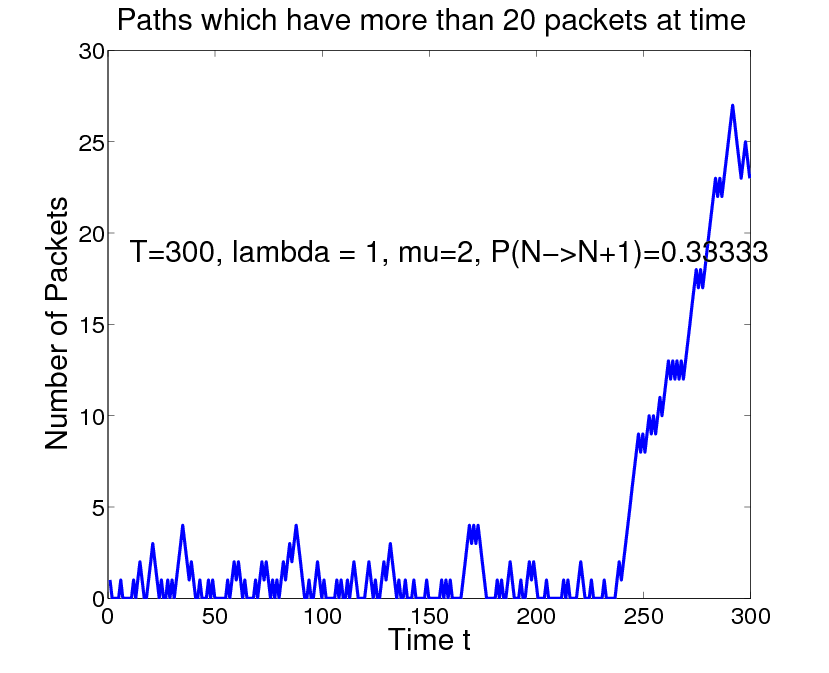
Our group is seeking ways to find rare events without solving the large deviation problem first. The picture below was produced using a histogram bisection strategy. Suppose X represents a configuration of some complex random system and we want to know the probability that f(X) > A, when this event is very small. Our method proceeds by repeated bifurcation of the histogram. The first step finds the median of the histogram, which is the number M1 so that the probability of f(X)>M1 is equal to .5. The next stage is to refine this top half to find M2 so that the probability that f(X)>m2 is .25. We do this not by direct simulation, but by a Metropolis type sampler that rejects configurations X that fall outside f(X)>.5. In the figure below, this bifurcation process was repeated 20 times, giving paths whose probability is less than one in a million. The whole process took well under a million path simulations. The large deviation theory for this problem is known and the path below is typical of what large deviations predicts such paths should look like.