G22.2130: Compiler Construction
2008-09 Spring
Allan Gottlieb
Tuesdays 5-6:50 CIWW 109
Start Lecture #1
Chapter 0: Administrivia
I start at Chapter 0 so that when we get to chapter 1, the
numbering will agree with the text.
0.1: Contact Information
- <my-last-name> AT nyu DOT edu (best method)
- http://cs.nyu.edu/~gottlieb
- 715 Broadway, Room 712
- 212 998 3344
0.2: Course Web Page
There is a web site for the course.
You can find it from my home page listed above.
- You can also find these lecture notes on the course home page.
Please let me know if you can't find it.
- The notes are updated as bugs are found or improvements made.
- I will also produce a separate page for each lecture after the
lecture is given.
These individual pages might not get updated as quickly as the
large page.
0.3: Textbook
The course text is Aho, Lam, Sethi, and Ullman:
Compilers: Principles, Techniques, and Tools,
second edition
- Available in bookstore.
- We will cover most of the first 8 chapters (plus some asides).
- The first edition is a descendant of the classic
Principles of Compiler Design.
- Independent of the titles, each of the books is called
The Dragon Book
, due to the cover picture.
0.4: Computer Accounts and Mailman Mailing List
- You are entitled to a computer account on one of the departmental
sun machines.
If you do not have one already, please get it asap.
- Sign up for the Mailman mailing list for the course.
You can do so by clicking
here
- If you want to send mail just to me, use the address given
above, not the mailing list.
- Questions on the labs should go to the mailing list.
You may answer questions posed on the list as well.
Note that replies are sent to the list.
- I will respond to all questions; if another student has answered the
question before I get to it, I will confirm if the answer given is
correct.
- Please use proper mailing list etiquette.
- Send plain text messages rather than (or at least in
addition to) html.
- Use the Reply command to contribute to the current thread,
but NOT to start another topic.
- If quoting a previous message, trim off irrelevant parts.
- Use a descriptive Subject: field when starting a new topic.
- Do not use one message to ask two unrelated questions.
- Do NOT make the mistake of sending your completed lab
assignment to the mailing list.
This is not a joke; several students have made this mistake in
past semesters.
0.5: Grades
Your grade will be a function of your final exam and laboratory
assignments (see below).
I am not yet sure of the exact weightings
for each lab and the final, but the final will be roughly half the
grade (very likely between 40% and 60%).
0.6: The Upper Left Board
I use the upper left board for lab/homework assignments and
announcements.
I should never erase that board.
If you see me start to erase an announcement, please let me know.
I try very hard to remember to write all announcements on the upper
left board and I am normally successful.
If, during class, you see
that I have forgotten to record something, please let me know.
HOWEVER, if I forgot and no one reminds me, the
assignment has still been given.
0.7: Homeworks and Labs
I make a distinction between homeworks and labs.
Labs are
- Required.
- Due several lectures later (date given on assignment).
- Graded and form part of your final grade.
- Penalized for lateness.
- Most often are computer programs you must write.
Homeworks are
- Optional.
- Due the beginning of the Next lecture.
- Not accepted late.
- Mostly from the book.
- Collected and returned.
- Able to help, but not hurt, your grade.
0.7.1: Homework Numbering
Homeworks are numbered by the class in which they are assigned.
So any homework given today is homework #1.
Even if I do not give homework today, the homework assigned next
class will be homework #2.
Unless I explicitly state otherwise, all homeworks assignments can
be found in the class notes.
So the homework present in the notes for lecture #n is homework #n
(even if I inadvertently forgot to write it to the upper left
board).
0.7.2: Doing Labs on non-NYU Systems
You may solve lab assignments on any system you wish, but ...
- You are responsible for any non-nyu machine.
I extend deadlines if the nyu machines are down, not if yours are.
- Be sure test your assignments to the nyu
systems.
In an ideal world, a program written in a high level language
like Java, C, or C++ that works on your system would also work
on the NYU system used by the grader.
Sadly this ideal is not always achieved despite marketing
claims to the contrary.
So, although you may develop you lab on any system,
you must ensure that it runs on the nyu system assigned to the
course.
- If somehow your assignment is misplaced by me and/or a grader,
we need a to have a copy ON AN NYU SYSTEM
that can be used to verify the date the lab was completed.
- When you complete a lab and have it on an nyu system, email the
lab to the grader and copy yourself on that message.
This email must come from your CIMS account.
Keep the copy until you have received your grade on the
assignment.
The systems support staff can retrieve your mail from their logs
given your copy and from that we can verify the dates.
I realize that I am being paranoid about this.
It is rare for labs to get misplaced, but they sometimes do and I
really don't want to be in the middle of an
I sent it ... I never received it
debate.
Thank you.
0.7.3: Obtaining Help with the Labs
Good methods for obtaining help include
- Asking me during office hours (see web page for my hours).
- Asking the mailing list.
- Asking another student, but ...
- ... Your lab must be your own.
That is, each student must submit a unique lab.
Naturally, simply changing comments, variable names, etc. does
not produce a unique lab.
See the Academic Integrity Policy below.
0.7.4: Computer Language Used for Labs
You may write your lab in Java, C, or C++.
Other languages may be possible, but please ask in advance.
I need to ensure that the TA is comfortable with the language.
0.8: A Grade of Incomplete
The rules for incompletes and grade changes are set by the school
and not the department or individual faculty member.
The rules set by GSAS state:
The assignment of the grade Incomplete Pass(IP)
or Incomplete Fail(IF) is at the discretion of
the instructor.
If an incomplete grade is not
changed to a permanent grade by the instructor
within one year of the beginning of the course,
Incomplete Pass(IP) lapses to No Credit(N), and
Incomplete Fail(IF) lapses to Failure(F).
Permanent grades may not be changed unless the
original grade resulted from a clerical error.
0.9: An Introductory Compiler Course with a Programming Prerequisite
0.9.1: An Introductory Course ...
I do not assume you have had a compiler course as an undergraduate,
and I do not assume you have had experience
developing/maintaining a compiler.
If you have already had a compiler class,
this course is probably not appropriate.
For example, if you can explain the following concepts/terms,
the course is probably too elementary for you.
- Parsing
- Lexical Analysis
- Syntax analysis
- Register allocation
- LALR Grammar
0.9.2: ... with a Programming Prerequisite
I do assume you are an experienced programmer.
There will be
non-trivial programming assignments during this course.
Indeed, you
will write a compiler for a simple programming language.
I also assume that you have at least a passing familiarity with
assembler language.
In particular, your compiler may need to produce
assembler language, but probably it will produce an
intermediate language consisting of
3-address code.
We will also be using addressing modes found in typical assemblers.
We will not, however, write significant
assembly-language programs.
0.10: Academic Integrity Policy
This email from the assistant director, describes the policy.
    Dear faculty,

    The vast majority of our students comply with the
    department's academic integrity policies; see

      www.cs.nyu.edu/web/Academic/Undergrad/academic_integrity.html
      www.cs.nyu.edu/web/Academic/Graduate/academic_integrity.html

    Unfortunately, every semester we discover incidents in
    which students copy programming assignments from those of
    other students, making minor modifications so that the
    submitted programs are extremely similar but not identical.

    To help in identifying inappropriate similarities, we
    suggest that you and your TAs consider using Moss, a
    system that automatically determines similarities between
    programs in several languages, including C, C++, and Java.
    For more information about Moss, see:

      http://theory.stanford.edu/~aiken/moss/

    Feel free to tell your students in advance that you will be
    using this software or any other system.  And please emphasize,
    preferably in class, the importance of academic integrity.

    Rosemary Amico
    Assistant Director, Computer Science
An Interlude from Chapter 2
I present this snippet from chapter 2 here (it appears where
it belongs
as well), since it is self-contained and is needed
for lab number 1, which I wish to assign today.
2.3.4: (depth-first) Tree Traversals
When performing a depth-first tree traversal, it is clear in what
order the leaves are to be visited, namely left to right.
In contrast there are several choices as to when to
visit an interior (i.e. non-leaf) node.
The traversal can visit an interior node
- Before visiting any of its children.
- Between visiting its children.
- After visiting all of its children.
I do not like the book's pseudocode as I feel the names chosen confuse
the traversal with visiting the nodes.
I prefer the pseudocode below, which uses the following conventions.
- Comments are introduced by -- and terminate at the end of the
line (as in the programming language Ada).
- Indenting is significant so begin/end or {} are not used (from
the programming language family B2/ABC/Python)
  traverse (n : treeNode)
      if leaf(n)                      -- visit leaves once; base of recursion
         visit(n)
      else                            -- interior node, at least 1 child
         -- visit(n)                  -- visit node PRE visiting any children
         traverse(first child)        -- recursive call
         while (more children remain) -- excluding first child
             -- visit(n)              -- visit node IN-between visiting children
             traverse (next child)    -- recursive call
         -- visit(n)                  -- visit node POST visiting all children
Note the following properties
-
As written, with the last three visit()s commented out, only
the leaves are visited and those visits are in left to right
order.
-
If you uncomment just the first (interior node) visit, you
get a preorder traversal, in which each node is
visited before (i.e., pre) visiting any of its
children.
-
If you uncomment just the last visit, you get a
postorder traversal, in which each node is visited
after (i.e., post) visiting all of its children.
-
If you uncomment only the middle visit, you get an
inorder traversal, in which the node is visited (in-)
between visiting its children.
Inorder traversals are normally defined only for binary trees,
i.e., trees in which every interior node has exactly two
children.
Although the code with only the middle visit uncommented
works
for any tree, we will, like everyone else,
reserve the name inorder traversal
for binary trees.
In the case of binary search trees
(everything in the left subtree is smaller than the root of
that subtree, which in tern is smaller than everything in the
corresponding right subtree) an inorder traversal visits the
values of the nodes in (numerical) order.
-
If you uncomment two of the three visits, you get a traversal
without a name.
-
If you uncomment all of the three visits, you get an
Euler-tour traversal.
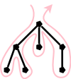
To explain the name Euler-tour traversal, recall that
an Eulerian tour on a directed graph is one that traverses
each edge once.
If we view the tree on the right as undirected and replace each edge
with two arcs, one in each direction, we see that the pink curve is
indeed an Eulerian tour.
It is easy to see that the curve visits the nodes in the order of
the pseudocode (with all visits uncommented).
Normally, the Euler-tour traversal is defined only for a binary
tree, but this time I will differ from convention and use
the pseudocode above to define Euler-tour traversal for all
trees.
Note the following points about our Euler-tour traversal.
- A node with k children is visited k+1 times.
The diagram shows nodes with 0, 1, 2, and 3 children.
- In a binary tree, a leaf is visited once and an
interior node is visited three times.
This is one of the standard definitions of an Euler-tour
traversal for a binary tree.
- The other standard definition has all nodes visited 3
times.
For a leaf the three visits are in succession.
Modifying the pseudocode to obtain this definition simply
requires replacing the
leaf visit
with
visit(n); visit(n); visit(n)
Do the Euler-tour traversal for the tree in the notes and then for
a binary tree.
Lab 1 assigned. See the home page.
Roadmap of the Course
- Chapter 1 touches on all the material.
- Chapter 2 constructs (the front end of) a simple compiler.
- Chapters 3-8 fill in the (considerable) gaps, as well as
the presenting the beginnings of the compiler back end.
I always spend too much time on introductory chapters, but will try
not to.
I have said this before.
Chapter 1: Introduction to Compiling
Homework Read chapter 1.
1.1: Language Processors
A Compiler is a translator from one language, the input
or source language, to another language, the output
or target language.
Often, but not always, the target language is an assembler language
or the machine language for a computer processor.
Note that using a compiler requires a two step process to run a
program.
- Execute the compiler (and possibly an assembler) to translate
the source program into a machine language program.
- Execute the resulting machine language program, supplying
appropriate input.
This should be compared with an interpreter, which accepts
the source language program and the appropriate
input, and itself produces the program output.
Sometimes both compilation and interpretation are used.
For example, consider typical Java implementations.
The (Java) source code is translated (i.e., compiled)
into bytecodes, the machine language for an
idealized virtual machine
, the Java Virtual Machine or JVM.
Then an interpreter of the JVM (itself normally called a JVM)
accepts the bytecodes and the appropriate input,
and produces the output.
This technique was quite popular in academia some time ago with the
Pascal programming language and P-code.
Homework: 1, 2, 4
Remark: Unless otherwise stated, homeworks are
from the book and specifically from the end of the second level
section we are discussing.
Even more specifically, we are in section 1.1, so you are to do the
first, second, and fourth problem at the end of section 1.1.
These three problems are numbered 1.1.1, 1.1.2, and 1.1.4 in the
book.
The compilation tool chain
For large programs, the compiler is actually part of a multistep
tool chain
[preprocessor] → [compiler] → [assembler]
→ [linker] → [loader]
We will be primarily focused on the second element of the chain,
the compiler.
Our target language will be assembly language.
I give a very short description of the other components, including
some historical comments.
Preprocessors
Preprocessors are normally fairly simple as in the C language,
providing primarily the ability to include files and expand macros.
There are exceptions, however.
IBM's PL/I, another Algol-like language had quite an extensive
preprocessor, which made available at preprocessor time, much of the
PL/I language itself (e.g., loops and I believe procedure calls).
Some preprocessors essentially augment the base language, to add
additional capabilities.
One could consider them as compilers in their own right, having as
source this augmented language (say Fortran augmented with
statements for multiprocessor execution in the guise of Fortran
comments) and as target the original base language (in this case
Fortran).
Often the preprocessor
inserts procedure calls to
implement the extensions at runtime.
Assemblers
Assembly code is an mnemonic version of machine code in which
names, rather than binary values, are used for machine instructions,
and memory addresses.
Some processors have fairly regular operations and as a result
assembly code for them can be fairly natural and not-too-hard to
understand.
Other processors, in particular Intel's x86 line, have let us
charitably say more interesting
instructions with certain
registers used for certain things.
My laptop has one of these latter processors (pentium 4) so my gcc
compiler produces code that from a pedagogical viewpoint is less
than ideal.
If you have a mac with a ppc processor (newest macs are x86), your
assembly language is cleaner.
NYU's ACF features sun computers with sparc processors, which also
have regular instruction sets.
Two pass assembly
No matter what the assembly language is, an assembler needs to
assign memory locations to symbols (called identifiers) and use the
numeric location address in the target machine language produced.
Of course the same address must be used for all occurrences of a
given identifier and two different identifiers must (normally) be
assigned two different locations.
The conceptually simplest way to accomplish this is to make two
passes over the input (read it once, then read it again from the
beginning).
During the first pass, each time a new identifier is encountered,
an address is assigned and the pair (identifier, address) is
stored in a symbol table.
During the second pass, whenever an identifier is encountered, its
address is looked up in the symbol table and this value is used in
the generated machine instruction.
Linkers
Linkers, a.k.a. linkage editors combine the output of the
assembler for several different compilations.
That is the horizontal line of the diagram above should really be
a collection of lines converging on the linker.
The linker has another input, namely libraries, but to the linker
the libraries look like other programs compiled and assembled.
The two primary tasks of the linker are
- Relocating relative addresses.
- Resolving external references (such as the procedure xor() above).
Relocating relative addresses
The assembler processes one file at a time.
Thus the symbol table produced while processing file A is
independent of the symbols defined in file B, and conversely.
Thus, it is likely that the same address will be used for
different symbols in each program.
The technical term is that the (local) addresses in the symbol
table for file A are relative to file A; they must
be relocated by the linker.
This is accomplished by adding the starting address of file A
(which in turn is the sum of the lengths of all the files
processed previously in this run) to the relative address.
Resolving external references
Assume procedure f, in file A, and procedure g, in file B, are
compiled (and assembled) separately.
Assume also that f invokes g.
Since the compiler and assembler do not see g when processing f,
it appears impossible for procedure f to know where in memory to
find g.
The solution is for the compiler to indicated in the output of
the file A compilation that the address of g is needed.
This is called a use of g.
When processing file B, the compiler outputs the (relative)
address of g.
This is called the definition of g.
The assembler passes this information to the linker.
The simplest linker technique is to again make two passes.
During the first pass, the linker records in its
external symbol table
(a table of external symbols, not a
symbol table that is stored externally) all the definitions
encountered.
During the second pass, every use can be resolved by access to the
table.
I cover the linker in more detail when I teach 2250, OS Design.
You can find my class notes for OS Design starting at my home
page.
Loaders
After the linker has done its work, the resulting
executable file
can be loaded by the operating system into
central memory.
The details are OS dependent.
With early single-user operating systems all programs would be
loaded into a fixed address (say 0) and the loader simply copies
the file to memory.
Today it is much more complicated since (parts of) many programs
reside in memory at the same time.
Hence the compiler/assembler/linker cannot know the real
location for an identifier.
Indeed, this real location can change.
More information is given in many OS courses.
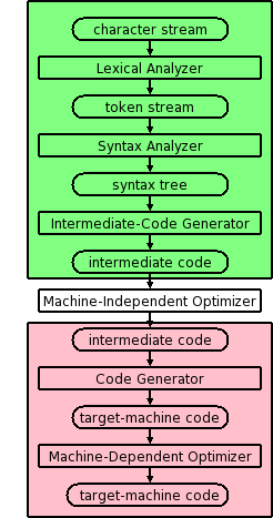
1.2: The Structure of a Compiler
Modern compilers contain two (large) parts, each of which is often
subdivided.
These two parts are the front end, shown in green on the right
and the back end, shown in pink.
The front end analyzes the source program, determines its
constituent parts, and constructs an intermediate representation of
the program.
Typically the front end is independent of the target language.
The back end synthesizes the target program from the
intermediate representation produced by the front end.
Typically the back end is independent of the source language.
This front/back division very much reduces the work for a compiling
system that can handle several (N) source languages and several (M)
target languages.
Instead of NM compilers, we need N front ends and M back ends.
For gcc (originally abbreviating Gnu C Compiler
, but
now abbreviating Gnu Compiler Collection
), N=7 and
M~30 so the savings are considerable.
Other analyzers and synthesizers
Other compiler like
applications also use analysis and
synthesis. Some examples include
- Pretty printer: Can be considered a real compiler with the
target language a formatted version of the source.
- Interpreter.
The synthesis traverses the intermediate code and executes the
operation at each node (rather than generating machine code to
do such).
Multiple Phases
The front and back end are themselves each divided into
multiple phases.
Conceptually, the input to each phase is the output of the previous.
Sometime a phase changes the representation of the input.
For example, the lexical analyzer converts a character stream input
into a token stream output.
Sometimes the representation is unchanged.
For example, the machine-dependent optimizer transforms
target-machine code into (hopefully improved) target-machine code.
The diagram is definitely not drawn to scale, in terms of effort or
lines of code.
In practice, the optimizers dominate.
Conceptually, there are three phases of analysis with the output of
one phase the input of the next.
Each of these phases changes the representation of the program being
compiled.
The phases are called lexical analysis or
scanning, which transforms the program from a string of
characters to a string of tokens; syntax analysis
or parsing, which transforms the program from a string of
tokens to some kind of syntax tree; and semantic analysis,
which decorates
the tree with semantic information.
Note that the above classification is conceptual; in practice more
efficient representations may be used.
For example, instead of having all the information about the program
in the tree, tree nodes may point to symbol table entries.
Thus the information about the variable X is stored
once and pointed to at each occurrence.
1.2.1: Lexical Analysis (or Scanning)
The character stream input is grouped into meaningful units
called lexemes, which are then mapped
into tokens, the latter constituting the output of
the lexical analyzer.
For example, any one of the following C statements
    x3 := y + 3;
    x3  :=   y   +   3   ;
    x3   :=y+ 3  ;
but not
x 3 := y + 3;
would be grouped into the lexemes x3, :=, y, +, 3, and ;.
A token is a <token-name,attribute-value> pair.
For example
- The lexeme x3 would be mapped to a token such as <id,1>.
The name id is short for identifier.
The value 1 is the index of the entry for x3 in the symbol table
produced by the compiler.
This table is used gather information about the identifiers and
to pass this information to subsequent phases.
- The lexeme := would be mapped to the token <:=>.
In reality it is probably mapped to a pair, whose second
component is ignored.
The point is that there are many different identifiers so we
need the second component, but there is only one assignment
symbol :=.
- The lexeme y is mapped to the token <id,2>
- The lexeme + is mapped to the token <+>.
- The lexeme 3 is somewhat interesting and is discussed further
in subsequent chapters.
It is mapped to <number,something>, but what is the
something.
On the one hand there is only one 3 so we could just use the
token <number,3>.
However, there can be a difference between how this should be
printed (e.g., in an error message produced by subsequent
phases) and how it should be stored (fixed vs. float vs. double).
Perhaps the token should point to the symbol table where an
entry for
this kind of 3
is stored.
Another possibility is to have a separate numbers table
.
- The lexeme ; is mapped to the token <;>.
- Lexemes are often described by regular expressions,
which we shall study in detail later in this course.
Note that non-significant blanks are normally removed during
scanning.
In C, most blanks are non-significant.
That does not mean the blanks are unnecessary.
Consider
    int x;
    intx;
The blank between int and x is clearly necessary, but it is not part
of any lexeme.
Blanks inside strings are an exception, they are part of the lexeme
and the corresponding token (or more likely the table entry pointed
to by the second component of the token).
Note that we can define identifiers, numbers, and the various
symbols and punctuation without using recursion (compare
with parsing below).
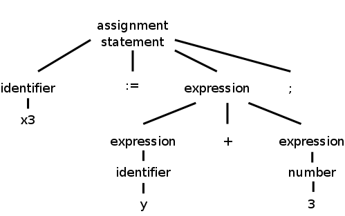
1.2.2: Syntax Analysis (or Parsing)
Parsing involves a further grouping in which tokens are grouped
into grammatical phrases, which are often represented in a parse
tree (also called a concrete syntax tree).
For example
x3 := y + 3;
would be parsed into the tree on the right.
This parsing would result from a grammar containing rules such as
    asst-stmt → id := expr ;
    expr      → number
              |  id
              |  expr + expr
Note the recursive definition of expression (expr). Note also the
hierarchical decomposition in the figure on the right.
The division between scanning and parsing is somewhat arbitrary, in
that some tasks can be accomplished by either.
However, if a recursive definition is involved (as it is above for
expr, it is considered parsing not scanning.
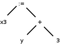
Often one uses a simpler tree called the syntax tree
(more properly the abstract syntax tree) with operators as
interior nodes and operands as the children of the operator.
The syntax tree on the right corresponds to the parse tree above it.
We expand on this point later.
(Technical point.)
The syntax tree shown represents an assignment expression not an
assignment statement.
In C an assignment statement includes the trailing semicolon.
That is, in C (unlike in Algol) the semicolon is a statement
terminator not a statement separator.
1.2.3: Semantic Analysis
There is more to a front end than simply syntax.
The compiler needs semantic information, e.g., the types (integer,
real, pointer to array of integers, etc) of the objects involved.
This enables checking for semantic errors and inserting type
conversion where necessary.
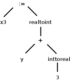
For example, if y was declared to be a real and x3 an integer, we
need to insert (unary, i.e., one operand) conversion operators
inttoreal
and realtoint
as shown on the right.
In this class we will use three-address-code for our intermediate
language; another possibility that is used is some kind of syntax
tree.
1.2.4: Intermediate code generation
Many compilers internally generate intermediate code for an
idealized machine
.
For example, the intermediate code generated would assume that the
target has an unlimited number of registers and that any register
can be used for any operation.
This is similar to a machine model with no registers, but
which permits operations to be directly performed on memory
locations.
Another common assumption is that machine operations take (up to)
three operands: two source and one target.
With these assumptions of a machine with an unlimited number of
registers and instructions with three operands, one generates
three-address code
by walking the semantic tree.
Our example C instruction would produce
    temp1 = inttoreal(3)
    temp2 = y + temp1
    temp3 = realtoint(temp2)
    x3 = temp3
We see that three-address code can include instructions
with fewer than 3 operands.
Sometimes three-address code is called quadruples because one can
view the previous code sequence as
    inttoreal temp1 3     --
    add       temp2 y     temp1
    realtoint temp3 temp2 --
    assign    x3    temp3 --
Each quad
has the form
operation target source1 source2
1.2.5: Code optimization
This is a very serious subject, one that we will not really
do justice to in this introductory course.
Some optimizations, however, are fairly easy to understand.
- Since 3 is a constant, the compiler can perform the int to
real conversion and replace the first two quads with
add temp2 y 3.0
- The last two quads can be combined into
realtoint x3 temp2
In addition to optimizations performed on the intermediate code,
further optimizations can be performed on the machine code by the
machine-dependent back end.
1.2.6: Code generation
Modern processors have only a limited number of register.
Although some processors, such as the x86, can perform operations
directly on memory locations, we will for now assume only register
operations.
Some processors (e.g., the MIPS architecture) use three-address
instructions.
We follow this model.
Other processors permit only two addresses; the result overwrites
one of the sources.
Using three-address instructions restricted to registers (except for
load and store instructions, which naturally must also reference
memory), code something like the following would be produced for our
example, after first assigning memory locations to x3 and y.
    LD   R1,  y
    LD   R2,  #3.0        // Some would allow constant in ADD
    ADDF R1,  R1, R2      // add float
    RTOI R2,  R1          // real to int
    ST   x3,  R2
1.2.7: Symbol-Table Management
The symbol table stores information about program variables
that will be used across phases.
Typically, this includes type information and storage locations.
A possible point of confusion: the storage location
does not give the location where the compiler has
stored the variable.
Instead, it gives the location where the compiled program will store
the variable.
1.2.8: The Grouping of Phases into Passes
Logically each phase is viewed as a separate pass, i.e., a
program that reads input and produces output for the next phase.
The phases thus form a pipeline.
In practice some phases are combined into a single pass.
For example one could have the entire front end as one pass.
The term pass is used to indicate that the entire
input is read during this activity.
So two passes, means that the input is read twice.
A grayed out (optional) portion of the notes above discusses 2-pass
approaches for both assemblers
and linkers.
If we implement each phase separately and possibly use multiple
passes for some of them, the compiler will perform a large number of
I/O operations, an expensive undertaking.
As a result, techniques have been developed to reduce the number of
passes.
We will see in the next chapter how to combine the scanner, parser,
and semantic analyzer into one program or phase.
Consider the parser.
When it needs to input the next token, rather than reading the input
file (presumably produced by the scanner), the parser calls the
scanner instead.
At selected points during the production of the syntax tree, the
parser calls the intermediate-code generator
which performs
semantic analysis as well as generating a portion of the
intermediate code.
For pedagogical reasons, we will not be employing this technique.
That is to ease the programming and understanding, we will use a
compiler design that performs more I/O than necessary.
Naturally, production compilers do not do this.
Thus, your compiler will consist of separate programs for
the scanner, parser, and semantic analyzer / intermediate code
generator.
Indeed, these will likely be labs 2, 3, and 4.
Reducing the Number of Passes
One problem with combining phases, or with implementing a single
phase in one pass, is that it appears that an internal form of the
entire program being compiled will need to be stored in memory.
This problem arises because the downstream phase may need, early in
its execution, information that the upstream phase produces only
late in its execution.
This motivates the use of symbol tables and a two pass approach in
which the symbol table is produced during the first pass and used
during the second pass.
However, a clever one-pass approach is often possible.
Consider an assembler (or linker).
The good case is when a symbol definition precedes all its uses so
that the symbol table contains the value of the symbol prior to that
value being needed.
Now consider the harder case of one or more uses preceding the
definition.
When a not-yet-defined symbol is first used, an entry is placed in
the symbol table, pointing to this use and indicating that the
definition has not yet appeared.
Further uses of the same symbol attach their addresses to a linked
list of undefined uses
of this symbol.
When the definition is finally seen, the value is placed in the
symbol table, and the linked list is traversed inserting the value
in all previously encountered uses.
Subsequent uses of the symbol will find its definition in the table.
This technique is called backpatching.
1.2.9: Compiler-construction tools
Originally, compilers were written from scratch
, but now the
situation is quite different.
A number of tools are available to ease the burden.
We will mention tools that generate scanners and parsers.
This will involve us in some theory: regular expressions for
scanners and context-free grammars for parsers.
These techniques are fairly successful.
One drawback can be that they do not execute as fast as
hand-crafted
scanners and parsers.
We will also see tools for syntax-directed translation and
automatic code generation.
The automation in these cases is not as complete.
Finally, there is the large area of optimization.
This is not automated; however, a basic component of optimization is
data-flow analysis
(how values are transmitted between
parts of a program) and there are tools to help with this task.
Pedagogically, a problem with using the tools is that your effort
shifts from understanding how a compiler works to
how the tool is used.
So instead of studying regular expressions and finite state
automata, you study the flex man pages and user's
guide.
Error detection and reporting
As you have doubtless noticed, not all programming efforts
produce correct programs.
If the input to the compiler is not a legal source language
program, errors must be detected and reported.
It is often much easier to detect that the program is not legal
(e.g., the parser reaches a point where the next token cannot
legally occur) than to deduce what is the actual error (which may
have occurred earlier).
It is even harder to reliably deduce what the intended correct
program should be.
1.3: The Evolution of Programming Languages
1.3.1: The Move to Higher-level Languages
Assumed knowledge (only one page).
1.3.2: Impacts on Compilers
High performance compilers (i.e., the code generated performs well)
are crucial for the adoption of new language concepts and computer
architectures.
Also important is the resource utilization of the compiler itself.
Modern compilers are large.
On my laptop the compressed source of gcc is 38MB so uncompressed it
must be about 100MB.
1.4: The Science of Building a Compiler
1.4.1: Modeling in Compiler Design and Implementation
We will encounter several aspects of computer science during the
course.
Some, e.g., trees, I'm sure you already know well.
Other, more theoretical aspects, such as nondeterministic finite
automata, may be new.
1.4.2: The Science of Code Optimization
We will do very little optimization.
That topic is typically the subject of a second compiler course.
Considerable theory has been developed for optimization, but sadly
we will see essentially none of it.
We can, however, appreciate the pragmatic requirements.
- The optimizations must be correct (in all
cases).
- Performance must be improved for most programs.
- The increase in compilation time must be reasonable.
- The implementation effort must be reasonable.
1.5: Applications of Compiler Technology
1.5.1: Implementation of High-Level Programming Languages
- Abstraction: All modern languages support abstraction.
Data-flow analysis permits optimizations that significantly reduce
the execution time cost of abstractions.
- Inheritance: The increasing use of smaller, but more numerous,
methods has made interprocedural analysis important.
Also optimizations have improved virtual method dispatch.
- Array bounds checking in Java and Ada: Optimizations have been
produced that eliminate many checks.
- Garbage collection in Java: Improved algorithms.
- Dynamic compilation in Java: Optimizations to predict/determine
parts of the program that will be heavily executed and thus should
be the first/only parts dynamically compiled into native code.
1.5.2: Optimization for Computer Architectures
Parallelism
For 50+ years some computers have had multiple processors
internally.
The challenge with such multiprocessors
is to program
them effectively so that all the processors are utilized
efficiently.
Recently, multiprocessors have become commodity items, with
multiple processors (cores
) on a single chip.
Major research efforts have lead to improvements in
- Automatic parallelization: Examine serial programs to determine
and expose potential parallelism (points where different
parts of the computation can execute concurrently, i.e.,
in parallel
).
- Compilation of explicitly parallel languages.
Memory Hierarchies
All machines have a limited number of registers, which can be
accessed much faster than central memory.
All but the simplest compilers devote effort to using this scarce
resource effectively.
Modern processors have several levels of caches and advanced
compilers produce code designed to utilize the caches well.
1.5.3: Design of New Computer Architectures
RISC (Reduced Instruction Set Computer)
RISC computers have comparatively simple instructions, complicated
instructions require several RISC instructions.
A CISC, Complex Instruction Set Computer, contains both complex and
simple instructions.
A sequence of CISC instructions would be a larger sequence of RISC
instructions.
Advanced optimizations are able to find commonality in this larger
sequence and lower the total number of instructions.
The CISC Intel x86 processor line 8086/80286/80386/... had a major
implementation change with the 686 (a.k.a. pentium pro).
In this processor, the CISC instructions were decomposed into RISC
instructions by the processor itself.
Currently, code for x86 processors normally achieves highest
performance when the (optimizing) compiler emits primarily simple
instructions.
Specialized Architectures
A great variety has emerged.
Compilers are produced before the processors are
fabricated.
Indeed, compilation plus simulated execution of the generated
machine code is used to evaluate proposed designs.
1.5.4: Program Translations
Binary Translation
This means translating from one machine language to another.
Companies changing processors sometimes use binary translation to
execute legacy code on new machines.
Apple did this when converting from Motorola CISC processors to the
PowerPC.
An alternative to binary translation is to have the new processor
execute programs in both the new and old instruction set.
Intel had the Itanium processor also execute x86 code.
Digital Equipment Corp (DEC) had their VAX processor also execute
PDP-11 instructions.
Apple, does not produce processors so needed binary translation for
the MIPS→PowerPC transition
With the recent dominance of x86 processors, binary translators
from x86 have been developed so that other microprocessors can be
used to execute x86 software.
Hardware Synthesis
In the old days integrated circuits were designed by hand.
For example, the NYU Ultracomputer research group in the 1980s
designed a VLSI chip for rapid interprocessor coordination.
The design software we used essentially let you paint.
You painted blue lines where you wanted metal, green for
polysilicon, etc.
Where certain colors crossed, a transistor appeared.
Current microprocessors are much too complicated to permit such a
low-level approach.
Instead, designers write in a high level description language which
is compiled down the specific layout.
Database Query Interpreters
The optimization of database queries and transactions is quite a
serious subject.
Compiled Simulation
Instead of simulating a processor designs on many inputs, it may be
faster to compile the design first into a lower level
representation and then execute the compiled version.
1.5.5: Software Productivity Tools
Dataflow techniques developed for optimizing code are also useful
for finding errors.
Here correctness (finding all errors and only errors) is not a
requirement, which is a good thing since that problem is
undecidable.
Type Checking
Techniques developed to check for type correctness (we will see
some of these) can be extended to find other errors such as using an
uninitialized variable.
Bounds Checking
As mentioned above optimizations have been developed to eliminate
unnecessary bounds checking for languages like Ada and Java that
perform the checks automatically.
Similar techniques can help find potential buffer overflow
errors that can be a serious security threat.
Memory-Management Tools
Languages (e.g., Java) with garbage collection cannot have memory
leaks (failure to free no longer accessible memory).
Compilation techniques can help to find these leaks in languages
like C that do not have garbage collection.
1.6: Programming Language Basics
Skipped.
This is covered in our Programming Languages course, which is a
prerequisite for the Compilers course.
Remark: You should be able to do the exercises in
this section (but they are not assigned).
Chapter 2: A Simple Syntax-Directed Translator
Homework: Read chapter 2.
The goal of this chapter is to implement a very
simple compiler
.
Really we are just going as far as the intermediate code, i.e., the
front end.
Nonetheless, the output, i.e. the intermediate code, does look
somewhat like assembly language.
How is it possible to do this in just one chapter?
What is the rest of the book/course about?
In this chapter there is
- A simple source language.
- A target close to the source.
- No optimization.
- No machine-dependent back end.
- No tools.
- Little theory.
The material will be presented too fast for full understanding:
Starting in chapter 3, we slow down and explain everything.
Sometimes in chapter 2, we only show some of the possibilities
(typically omitting the hard cases) and don't even mention the
omissions.
Again, this is corrected in the remainder of the course.
A weakness of my teaching style is that I spend too long on
chapters like this.
I will try not to make that mistake this semester, but I have said
that before.
2.1: Introduction
We will be looking at the front end, i.e., the analysis
portion of a compiler.
The syntax describes the form of a program in a
given language, while the semantics describes
the meaning of that program.
We will learn the standard representation for the syntax,
namely context-free grammars also called BNF (Backus-Naur
Form).
We will learn syntax-directed translation, where the
grammar does more than specify the syntax.
We augment the grammar with attributes and use this to guide the
entire front end.
The front end discussed in this chapter has as source language
infix expressions consisting of digits, +, and -.
The target language is postfix expressions with the same components.
For example, the compiler will convert
7+4-5 to 74+5-.
Actually, our simple compiler will handle a few other operators as
well.
We will tokenize
the input (i.e., write a scanner), model
the syntax of the source, and let this syntax direct the translation
all the way to three-address code
, our intermediate language.
2.2: Syntax Definition
2.2.1: Definition of Grammars
This will be done right
in the next two chapters.
A context-free grammar (CFG) consists of
- A set of terminals (tokens produced by the lexer).
- A set of nonterminals.
- A set of productions (rules for transforming nonterminals).
These are written
LHS → RHS
where the LHS is a single nonterminal (that is
why this grammar is context-free) and the RHS is a
string containing nonterminals and/or terminals.
- A specific nonterminal designated as start symbol.
Example:
    Terminals: 0 1 2 3 4 5 6 7 8 9 + -
    Nonterminals: list digit
    Productions:
        list → list + digit
        list → list - digit
        list → digit
        digit → 0 | 1 | 2 | 3 | 4 | 5 | 6 | 7 | 8 | 9
    Start symbol: list
We use | to indicate that a nonterminal has multiple possible right
hand side.
So
A → B | C
is simply shorthand for
    A → B
    A → C
If no start symbol is specifically designated, the LHS of the first
production is the start symbol.
2.2.2: Derivations
Watch how we can generate the string 7+4-5 beginning with the start
symbol, applying productions, and stopping when no productions can
be applied (because only terminals remain).
    list → list - digit
         → list - 5
         → list + digit - 5
         → list + 4 - 5
         → digit + 4 - 5
         → 7 + 4 - 5
This process of applying productions, starting with the start
symbol and ending when only terminals are present is called a
derivation and we say that the final string has been
derived from the initial string (in this case the start
symbol).
The set of all strings derivable from the start symbol is the
language generated by the CFG
- It is important that you see that this context-free grammar
generates precisely the set of infix expressions with single digits
as operands (so 25 is not allowed) and + and - as operators.
- The way you get different final expressions is that you make
different choices of which production to apply. There are 3
productions you can apply to list and 10 you can apply to digit.
- The result cannot have blanks since blank is not a terminal.
- The empty string is not possible since, starting from list,
we cannot get to the empty string.
If we wanted to include the empty string, we would add the
production
list → ε
- The idea is that the input language to the compiler is
approximately the language generated by the grammar.
It is approximate since I have ignored the scanner.
Start Lecture #2
Given a grammar, parsing a string (of terminals) consists
of determining if the string is in the language generated by the
grammar.
If it is in the language, parsing produces a derivation.
If it is not, parsing reports an error.
The opposite of derivation is reduction.
Given a production, the LHS produces or derives the RHS (a
derivation) and the RHS is reduced to the LHS (a reduction).
Ignoring errors for the moment, parsing a string means reducing the
string to the start symbol or equivalently deriving
the string from the start symbol.
Homework: 1a, 1c, 2a-c (don't worry about
justifying
your answers).
Remark: Since we are in section 2.2 these
questions are in section 2.2.7, the last subsection of section
2.2.
2.2.3: Parse trees
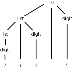
While deriving 7+4-5, one could produce the Parse Tree
shown on the right.
You can read off the productions from the tree.
For any internal (i.e., non-leaf) tree node, its children give the
right hand side (RHS) of a production having the node itself as the
LHS.
The leaves of the tree, read from left to right, is called the
yield of the tree.
We say that this string is derived from the (nonterminal at
the) root, or is generated by the root, or can be
reduced to the root.
The tree on the right shows that 7+4-5 can be derived from list.
Homework: 1b
2.2.4: Ambiguity
An ambiguous grammar is one in which there are two or more
parse trees yielding the same final string.
We wish to avoid such grammars.
The grammar above is not ambiguous.
For example 1+2+3 can be parsed only one way; the
arithmetic must be done left to right.
Note that I am not giving a rule of arithmetic, just of this
grammar.
If you reduced 2+3 to list you would be stuck since it is impossible
to further reduce 1+list (said another way it is not possible to
derive 1+list from the start symbol).
Remark:
The following is a wrong proof of ambiguity.
Consider the grammar
S → A B
A → x
B → x
This grammar is ambiguous because we can derive the string
x x in two ways
S → A B → A x → x x
S → A B → x B → x x
WRONG!!
There are indeed two derivations, but they have the same parse tree!
End of Remark.
Homework: 3 (applied only to parts a, b, and c of 2)
2.2.5: Associativity of operators
Our grammar gives left associativity.
That is, if you traverse the parse tree in postorder and perform the
indicated arithmetic you will evaluate the string left to right.
Thus 8-8-8 would evaluate to -8.
If you wished to generate right associativity (normally
exponentiation is right associative, so 2**3**2 gives 512 not 64),
you would change the first two productions to
  list → digit + list
  list → digit - list
Draw in class the parse tree for 7+4-5 with this new grammar.
2.2.6: Precedence of operators
We normally want * to have higher precedence than +.
We do this by using an additional nonterminal to indicate the items
that have been multiplied.
The example below gives the four basic arithmetic operations their
normal precedence unless overridden by parentheses.
Redundant parentheses are permitted.
Equal precedence operations are performed left to right.
  expr   → expr + term | expr - term | term
  term   → term * factor | term / factor | factor
  factor → digit | ( expr )
  digit  → 0 | 1 | 2 | 3 | 4 | 5 | 6 | 7 | 8 | 9
Do the examples 1+2/3-4*5 and (1+2)/3-4*5 on the board.
Note how the precedence is enforced by the grammar; slick!
Statements
Keywords are very helpful for distinguishing statements from one another.
    stmt → id := expr
    	 | if expr then stmt
    	 | if expr then stmt else stmt
    	 | while expr do stmt
    	 | begin opt-stmts end
    opt-stmts → stmt-list | ε
    stmt-list → stmt-list ; stmt | stmt
Remarks:
- In the above example I underlined the nonterminals.
This is not normally done.
It is easy to tell the nonterminals; they are the symbols that
appear on the LHS.
- opt-stmts stands for
optional statements
.
The begin-end block can be empty in some languages.
- The ε (epsilon) stands for the empty string.
- The use of
epsilon productions
will add complications.
- Some languages do not permit empty blocks.
For example, Ada has a
null
statement, which does nothing
when executed, but avoids the need for empty blocks.
- The above grammar is ambiguous!
- The notorious
dangling else
problem.
- How do you parse
if x then if y then z=1 else z=2
?
Homework: 4 a-d (for a the operands are digits and the
operators are +, -, *, and /).
2.3: Syntax-Directed Translation
The idea is to specify the translation of a source language
construct in terms of attributes of its syntactic components.
The basic idea is use the productions to specify a (typically
recursive) procedure for translation.
For example, consider the production
stmt-list → stmt-list ; stmt
To process the left stmt-list, we
- Call ourselves recursively to process the right stmt-list
(which is smaller).
This will, say, generate code for all the statements in the
right stmt-list.
- Call the procedure for stmt, generating code for stmt.
- Process the left stmt-list by combining the results for the
first two steps as well as what is needed for the semicolon (a
terminal, so we do not further delegate its actions).
In this case we probably concatenate the code for the right
stmt-list and stmt.
To avoid having to say the right stmt-list
and the left stmt-list
we write the production as
stmt-list → stmt-list1 ; stmt
where the subscript is used to distinguish the two instances of
stmt-list.
Question: Why won't this go on forever?
Answer: Eventually stmt-list1
will consist of only one stmt and then one of the other
production for stmt-list will be used.
2.3.1: Postfix Notation (An Example)
This notation is called postfix because the rule
is operator after operand(s)
.
Parentheses are not needed.
The notation we normally use is called infix because the
rules is operator in between operands
.
If you start with an infix expression, the following algorithm will
give you the equivalent postfix expression.
- Variables and constants are left alone.
- E op F becomes E' F' op, where E' and F' are the postfix of E
and F respectively.
- ( E ) becomes E', where E' is the postfix of E.
One question is, given say 1+2-3, what are E, F and op?
Does E=1+2, F=3, and op=-?
Or does E=1, F=2-3 and op=+?
This is the issue of precedence and associativity mentioned above.
To simplify the present discussion we will start with fully
parenthesized infix expressions.
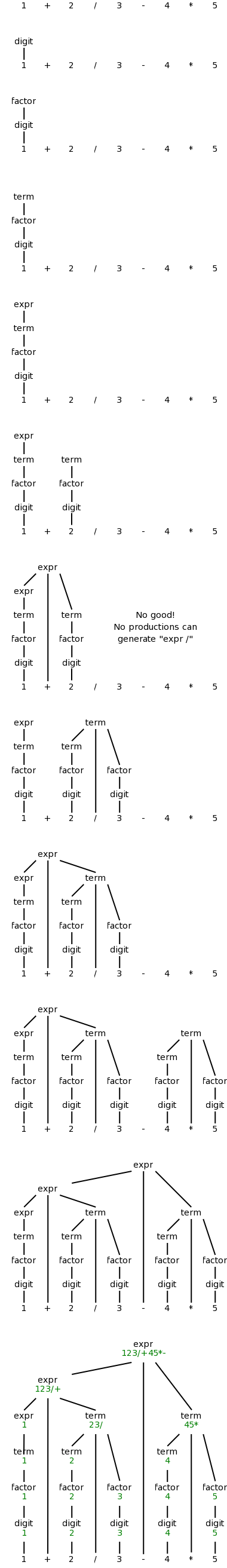
Example: 1+2/3-4*5
- Start with 1+2/3-4*5
- Parenthesize (using standard precedence) to get (1+(2/3))-(4*5)
- Apply the above rules to calculate P{(1+(2/3))-(4*5)}, where
P{X} means
convert the infix expression X to postfix
.
- P{(1+(2/3))-(4*5)}
- P{(1+(2/3))} P{(4*5)} -
- P{1+(2/3)} P{4*5} -
- P{1} P{2/3} + P{4} P{5} * -
- 1 P{2} P{3} / + 4 5 * -
- 1 2 3 / + 4 5 * -
Example: Now do (1+2)/3-4*5
- Parenthesize to get ((1+2)/3)-(4*5)
- Calculate P{((1+2)/3)-(4*5)}
- P{((1+2)/3) P{(4*5)} -
- P{(1+2)/3} P{4*5) -
- P{(1+2)} P{3} / P{4} P{5} * -
- P{1+2} 3 / 4 5 * -
- P{1} P{2} + 3 / 4 5 * -
- 1 2 + 3 / 4 5 * -
2.3.2: Synthesized Attributes
We want to decorate
the parse trees we construct with
annotations
that give the value of certain
attributes of the corresponding node of the tree.
Later in the semester, we will use as input an algol/ada/C-like
language and will have a code attribute for many nodes with
the property that code contains the intermediate code that
results from compiling the program corresponding to the leaves of
the subtree rooted at this node.
In particular,
the-root-of-the-parse-tree.code
will contain the compilation of the entire algol-like program.
However, it is now only the beginning of the semester so our goal
is more modest.
We will do the example of translating infix to postfix using the
same infix grammar as above.
For convenience, the grammar is repeated just below.
The names of the nonterminals correspond to standard arithmetic
terminology where one multiplies and divides factors to obtain
terms, which in turn are added and subtracted to form expressions.
  expr   → expr + term | expr - term | term
  term   → term * factor | term / factor | factor
  factor → digit | ( expr )
  digit  → 0 | 1 | 2 | 3 | 4 | 5 | 6 | 7 | 8 | 9
This grammar supports parentheses, although our example 1+2/3-4*5
does not use them.
On the right is a movie
in which the parse tree is built from
this example.
Question: Was this a top-down or bottom-up movie?
The attribute we will associate with the nodes is the postfix form
of the string in the leaves below the node.
In particular, the value of this attribute at the root is the
postfix form of the entire source.
The book does a simpler grammar (no *, /, or parentheses) for a
simpler example.
You might find that one easier.
Syntax-Directed Definitions (SDDs)
Definition: A syntax-directed definition
is a grammar together with semantic rules associated with
the productions.
These rules are used to compute attribute values.
A parse tree augmented with the attribute values at each node is
called an annotated parse tree.
For the bottom-up approach I will illustrate now, we annotate a
node after having annotated its children.
Thus the attribute values at a node can depend on the values of
attributes at the children of the node but not on attributes at the
parent of the node.
We call such bottom-up
attributes synthesized, since
they are formed by synthesizing the attributes of the children.
In chapter 5, when we study top-down annotations as well, we will
introduce inherited
attributes that are passed down from
parents to children.
We specify how to synthesize attributes by giving the semantic
rules together with the grammar.
That is, we give the syntax directed definition.
SDD for Infix to Posfix Translator
| Production | Semantic Rule |
|---|
| expr → expr1 + term
| expr.t := expr1.t || term.t || '+'
|
| expr → expr1 - term
| expr.t := expr1.t || term.t || '-'
|
| expr → term | expr.t := term.t |
| term → term1 * factor
| term.t := term1.t || factor.t || '*'
|
| term → term1 / factor
| term.t := term1.t || factor.t || '/'
|
| term → factor | term.t := factor.t |
| factor → digit | factor.t := digit.t |
| factor → ( expr ) | factor.t := expr.t |
| digit → 0 | digit.t := '0' |
| digit → 1 | digit.t := '1' |
| digit → 2 | digit.t := '2' |
| digit → 3 | digit.t := '3' |
| digit → 4 | digit.t := '4' |
| digit → 5 | digit.t := '5' |
| digit → 6 | digit.t := '6' |
| digit → 7 | digit.t := '7' |
| digit → 8 | digit.t := '8' |
| digit → 9 | digit.t := '9' |
We apply these rules bottom-up (starting with the geographically
lowest productions, i.e., the lowest lines in the tree) and get the
annotated graph shown on the right.
The annotation are drawn in green.
Homework: Draw the annotated graph for (1+2)/3-4*5.
2.3.3: Simple Syntax-Directed Definitions
If the semantic rules of a syntax-directed definition all have the
property that the new annotation for the left hand side (LHS) of the
production is just the concatenation of the annotations for the
nonterminals on the RHS in the same order as the nonterminals
appear in the production, we call the syntax-directed
definition simple.
It is still called simple if new strings are interleaved with the
original annotations.
So the example just done is a simple syntax-directed definition.
Remark: SDD's feature semantic rules.
We will soon learn about Translation Schemes, which feature a
related concept called semantic actions.
When one has a simple SDD, the corresponding translation scheme
can be done without constructing the parse tree.
That is, while doing the parse, when you get to the point where you
would construct the node, you just do the actions.
In the translation scheme corresponding to the present example,
the action at a node is just to print the new
strings at the appropriate points.
2.3.4: (depth-first) Tree Traversals
When performing a depth-first tree traversal, it is clear in what
order the leaves are to be visited, namely left to right.
In contrast there are several choices as to when to
visit an interior (i.e. non-leaf) node.
The traversal can visit an interior node
- Before visiting any of its children.
- Between visiting its children.
- After visiting all of its children.
I do not like the book's pseudocode as I feel the names chosen confuse
the traversal with visiting the nodes.
I prefer the pseudocode below, which uses the following conventions.
- Comments are introduced by -- and terminate at the end of the
line (as in the programming language Ada).
- Indenting is significant so begin/end or {} are not used (from
the programming language family B2/ABC/Python)
    traverse (n : treeNode)
        if leaf(n)                      -- visit leaves once; base of recursion
           visit(n)
        else                            -- interior node, at least 1 child
           -- visit(n)                  -- visit node PRE visiting any children
           traverse(first child)        -- recursive call
           while (more children remain) -- excluding first child
               -- visit(n)              -- visit node IN-between visiting children
               traverse (next child)    -- recursive call
           -- visit(n)                  -- visit node POST visiting all children
Note the following properties
- As written, with the last three visit()s commented out, only
the leaves are visited and those visits are in left to right
order.
- If you uncomment just the first (interior node) visit, you get
a preorder traversal, in which each node is visited
before (i.e., pre) visiting any of its children.
- If you uncomment just the last visit, you get a
postorder traversal, in which each node is visited
after (i.e., post) visiting all of its children.
- If you uncomment only the middle visit, you get an
inorder traversal, in which the node is visited (in-)
between visiting its children.
Inorder traversals are normally defined only for binary trees,
i.e., trees in which every interior node has exactly two
children.
Although the code with only the middle visit uncommented
works
for any tree, we will, like everyone else, reserve
the name inorder traversal
for binary trees.
In the case of binary search trees (everything
in the left subtree is smaller than the root of that subtree,
which in tern is smaller than everything in the corresponding
right subtree) an inorder traversal visits the values of the
nodes in (numerical) order.
- If you uncomment two of the three visits, you get a traversal
without a name.
- If you uncomment all of the three visits, you get an
Euler-tour traversal.
To explain the name Euler-tour traversal, recall that
an Eulerian tour on a directed graph is one that
traverses each edge once.
If we view the tree on the right as undirected and replace each
edge with two arcs, one in each direction, we see that the pink
curve is indeed an Eulerian tour.
It is easy to see that the curve visits the nodes in the order
of the pseudocode (with all visits uncommented).
Normally, the Euler-tour traversal is defined only for a binary
tree, but this time I will differ from convention and
use the pseudocode above to define Euler-tour traversal for all
trees.
Note the following points about our Euler-tour traversal.
Remarks
-
Since, at this point in the course, we are considering only
synthesized attributes, a postorder traversal will always yield a
correct evaluation order for the attributes.
This is so since synthesized attributes depend only on attributes of
child nodes and a postorder traversal visits a node only after all
the children have been visited (and hence all the child node
attributes have been evaluated).
-
In the general case (when not all attributes are synthesized), SDDs
do not specify an evaluation order for the attributes of the parse
tree.
The requirement remains that each attribute is evaluated after all
those that it depends on.
This general case is quite difficult, and sometimes no such order is
possible.
End of Remarks
2.3.5: Translation schemes
The bottom-up annotation scheme just described generates the final
result as the annotation of the root.
In our infix to postfix example we get the result desired by
printing the root annotation.
Now we consider another technique that produces its results
incrementally.
Instead of giving semantic rules for each production (and thereby
generating annotations) we can embed program fragments
called semantic actions within the productions themselves.
When drawn in diagrams (e.g., see the diagram below), the semantic
action is connected to its node with a distinctive, often dotted,
line.
The placement of the actions determine the order they are performed.
Specifically, one executes the actions in the order they are
encountered in a depth-first traversal of the tree (the children of
a node are visited in left to right order).
Note that these action nodes are all leaves and hence they are
encountered in the same order for both preorder and postorder
traversals (and inorder and Euler-tree order).
Definition: A
syntax-directed translation scheme is a context-free
grammar with embedded semantic actions.
In the SDD for our infix to postfix translator, the parent
either
- takes the attribute of its only child or
- concatenates the attributes left to right of its several
children and adds something at the end.
The equivalent semantic actions is to either print nothing or
print the new item.
Emitting a Translation
Semantic Actions and Rules for an Infix to Postfix Translator
| Production with Semantic Action
| Semantic Rule
|
|
|
| expr → expr1 + term
| { print('+') }
| expr.t := expr1.t || term.t || '+'
|
| expr → expr1 - term
| { print('-') }
| expr.t := expr1.t || term.t || '-'
|
| term → term1 / factor
| { print('/') }
| term.t := term1.t || factor.t || '/'
|
| term → factor
| { null }
| term.t := factor.t
|
| digit → 3
| { print ('3') }
| digit.t := '3'
|
The table on the right gives the semantic actions corresponding to
a few of the rows of the table above.
Note that the actions are enclosed in {}.
The corresponding semantic rules are given as well.
It is redundant to give both semantic actions and semantic rules;
in practice, we use one or the other.
In this course we will emphasize semantic rules, i.e. syntax
directed definitions (SDDs).
I show both the rules and the actions in a few tables just so that
we can see the correspondence.
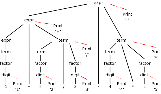
The diagram for 1+2/3-4*5 with attached semantic actions is shown
on the right.
Given an input, e.g. our favorite 1+2/3-4*5, we just do a
(left-to-right) depth first traversal of the corresponding diagram
and perform the semantic actions as they occur.
When these actions are print statements as above, we are said to be
emitting the translation.
Since the actions are all leaves of the tree, they occur in the
same order for any depth-first (left-to-right) traversal (e.g.,
postorder, preorder, or Euler-tour order).
Do on the board a depth first traversal of the diagram, performing
the semantic actions as they occur, and confirm that the translation
emitted is in fact 123/+45*-, the postfix version of 1+2/3-4*5
Homework: Produce the corresponding diagram for
(1+2)/3-4*5.
Prefix to infix translation
When we produced postfix, all the prints came at the end (so that
the children were already printed
).
The { action }'s do not need to come at the end.
We illustrate this by producing infix arithmetic (ordinary) notation
from a prefix source.
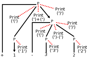
In prefix notation the operator comes first.
For example, +1-23 evaluates to zero and +-123 evaluates to 2.
Consider the following grammar, which generates the simple language
of prefix expressions consisting of addition and subtraction of
digits between 1 and 3 without parentheses (prefix notation and
postfix notation do not use parentheses).
P → + P P | - P P | 1 | 2 | 3
The resulting parse tree for +1-23 with the semantic actions
attached is shown on the right.
Note that the output language (infix notation) has
parentheses.
The table below shows both the semantic actions and rules used by
the translator.
As mentioned previously, one normally does not use both actions and
rules.
Prefix to infix translator
| Production with Semantic Action | Semantic Rule
|
|
|
| P → + { print('(') } P1 { print(')+(') }
P2 { print(')') }
| P.t := '(' || P1.t || ')+(' || P.t || ')'
|
|
|
| P → - { print('(') } P1 { print(')-(') }
P2 { print(')') }
| P.t := '(' || P1.t || ')-(' || P.t || ')'
|
|
|
| P → 1 { print('1') } | P.t := '1' |
|
|
| P → 2 { print('2') } | P.t := '2' |
|
|
| P → 3 { print('3') } | P.t := '3' |
First do a preorder traversal of the tree and see that you get
1+(2-3).
In fact you don't get that answer, but instead get a fully
parenthesized version that is equivalent.
Next start a postorder traversal and see that it produces the
same output (i.e., executes the same prints in the same order).
Question: What about an Euler-tour order?
Answer: The same result.
For all traversals, the leaves are printed in left
to right order and all the semantic actions are leaves.
Finally, pretend the prints aren't there, i.e., consider
the unannotated parse tree and perform
a postorder traversal, evaluating the semantic
rules at each node encountered.
Postorder is needed (and sufficient) since we have
synthesized attributes and hence having child attributes evaluated
prior to evaluating parent attributes is both necessary and
sufficient to ensure that whenever an attribute is evaluated all the
component attributes have already been evaluated.
(It will not be so easy in chapter 5, when we have inherited
attributes as well.)
Homework: 2.
2.4: Parsing
Objective:
Given a string of tokens and a grammar, produce a
parse tree yielding that string (or at least determine if such a
tree exists).
We will learn both top-down (begin with the start symbol, i.e. the
root of the tree) and bottom up (begin with the leaves) techniques.
In the remainder of this chapter we just do top down, which is
easier to implement by hand, but is less general.
Chapter 4 covers both approaches.
Tools (so called parser generators
) often use bottom-up
techniques.
In this section we assume that the lexical analyzer has already
scanned the source input and converted it into a sequence of
tokens.
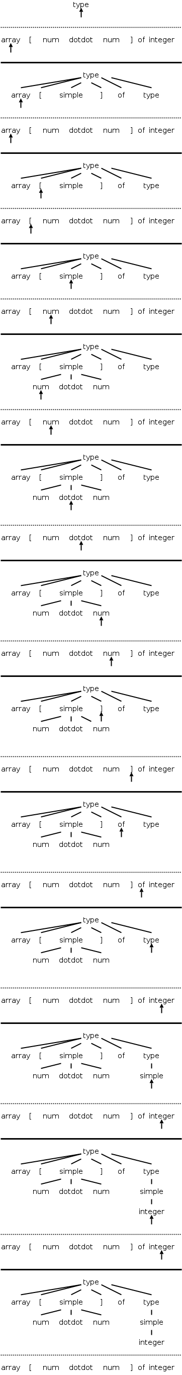
2.4.1: Top-down parsing
Consider the following simple language, which derives a subset
of the types found in the (now somewhat dated) programming language
Pascal.
I do not assume you know pascal.
We have two nonterminals, type, which is the start symbol, and
simple, which represents the simple
types.
There are 8 terminals, which are tokens produced by the lexer and
correspond closely with constructs in pascal itself.
Specifically, we have.
- integer and char
- id for identifier
- array and of used in array declarations
- ↑ meaning pointer to
- num for a (positive whole) number
- dotdot for .. (used to give a range like 6..9)
The productions are
    type   → simple
    type   → ↑ id
    type   → array [ simple ] of type
    simple → integer
    simple → char
    simple → num dotdot num
Parsing is easy in principle and for certain grammars (e.g., the
one above) it actually is easy.
We start at the root since this is top-down parsing and apply
the two fundamental steps.
- At the current (nonterminal) node, select a production whose LHS
is this nonterminal and whose RHS
matches
the input at this
point.
Make the RHS the children of this node (one child per RHS symbol).
- Go to the next node needing a subtree.
When programmed this becomes a procedure for each nonterminal that
chooses a production for the node and calls procedures for each
nonterminal in the RHS of that production.
Thus it is recursive in nature and descends the parse tree.
We call these parsers recursive descent
.
The big problem is what to do if the current node is the LHS of
more than one production.
The small problem is what do we mean by the next
node needing
a subtree.
The movie on the right, which succeeds in parsing, works by tossing
2 ounces of pixie dust into the air and choosing the production onto
which the most dust falls.
(An alternative interpretation is given below.)
The easiest solution to the big problem would be to assume that
there is only one production having a given nonterminal as LHS.
There are two possibilities
- No circularity. For example
	expr → term + term
	term → factor / factor
	factor → digit
	digit → 7
But this is very boring.
The only possible sentence is 7/7+7/7
- Circularity
	expr → term + term
	term → factor / factor
	factor → ( expr )
This is even worse; there are no (finite) sentences. Only an
infinite sentence beginning (((((((((.
So this won't work.
We need to have multiple productions with the same LHS.
How about trying them all?
We could do this!
If we get stuck where the current tree cannot match the input we are
trying to parse, we would backtrack.
Instead, we will look ahead one token in the input and only choose
productions that can yield a result starting with this token.
Furthermore, we will (in this section) restrict ourselves to
predictive parsing in which there is only one production
that can yield a result starting with a given token.
This solution to the big problem also solves the small problem.
Since we are trying to match the next token in the input, we must
choose the leftmost (nonterminal) node to give children to.
2.4.2: Predictive parsing
Let's return to pascal array type grammar and consider the three
productions having type as LHS.
Remember that, even when I write the short form
type → simple | ↑ id | array [ simple ] of type
we still have three productions.
For each production P we wish to construct the set FIRST(P)
consisting of those tokens (i.e., terminals) that can appear as the
first symbol of a string derived from the RHS of P.
FIRST is actually defined on strings not productions.
When I write FIRST(P), I really mean FIRST(RHS).
Similarly, I often say
the first set of the production P
when I should really say
the first set of the RHS of the production P
.
Formally, we proceed as follows.
Let α be a string of terminals and/or nonterminals.
FIRST(α) is the set of terminals that can appear as
the first symbol in a string of terminals derived from α.
If α is ε or α can derive ε, then
ε is in FIRST(α)
So given α we find all strings of terminals that can be
derived from α and pick off the first terminal from each
string (as often happens, ε requires a special case).
Question: How do we calculate FIRST(α)?
Answer: Wait until chapter 4 for a formal
algorithm.
For these simple examples it is reasonably clear.
Definition: Let r be the RHS of a production P.
FIRST(P) is FIRST(r).
To use predictive parsing, we make the following
Assumption: Let P and Q be two productions with
the same LHS,
Then FIRST(P) and FIRST(Q) are disjoint.
Thus, if we know both the LHS and the token that must be first, there
is (at most) one production we can apply.
BINGO!
An example of predictive parsing
This table gives the FIRST sets for our pascal array type example.
| Production | FIRST |
|---|
| type → simple | { integer, char, num } |
| type → ↑ id | { ↑ } |
| type → array [ simple ] of type | { array } |
| simple → integer | { integer } |
| simple → char | { char } |
| simple → num dotdot num | { num } |
Make sure that you understand how this table was
derived.
It is not yet clear how to calculate FIRST for a complicated
example.
We will learn the general procedure in chapter 4.
Note that the three productions with type as LHS have
disjoint FIRST sets.
Similarly the three productions with simple as LHS have
disjoint FIRST sets.
Thus predictive parsing can be used.
We process the input left to right and call the current
token lookahead since it is how far we are looking ahead in
the input to determine the production to use.
The movie on the right shows the process in action.
Homework:
A. Construct the FIRST sets for
    rest → + term rest | - term rest | term
    term → 1 | 2 | 3
B. Can predictive parsing be used?
End of Homework.
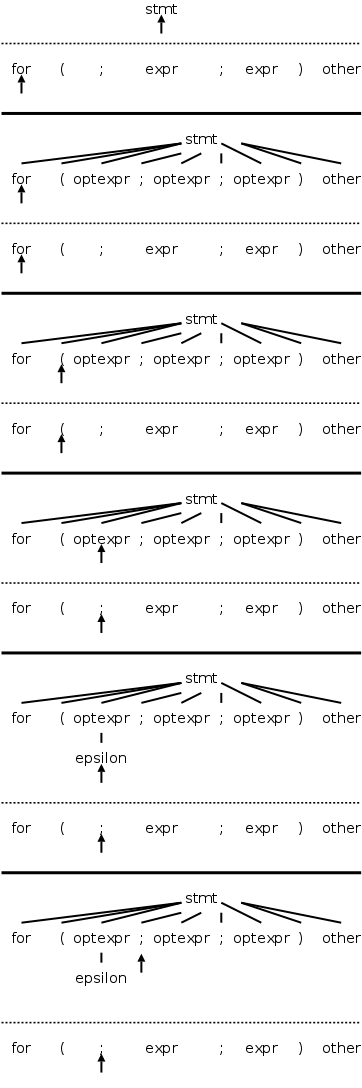
2.4.3: When to Use ε-productions
Not all grammars are as friendly as the last example. The first
complication is when ε occurs as a RHS. If this happens or
if the RHS can generate ε, then ε is included in
FIRST.
But ε would always match the current input position!
The rule is that if lookahead is not in FIRST of any production
with the desired LHS, we use the (unique!) production (with that
LHS) that has ε in FIRST.
The text does a C instead of a pascal example.
The productions are
    stmt → expr ;
    	 | if ( expr ) stmt
    	 | for ( optexpr ; optexpr ; optexpr ) stmt
    	 | other
    optexpr → expr | ε
For completeness, on the right is the beginning of a
movie for the C example.
Note the use of the ε-production at the end since no other
entry in FIRST will match ;
Once again, the full story will be revealed in chapter 4 when we do
parsing in a more complete manner.
2.4.4: Designing a Predictive Parser
Predictive parsers are fairly easy to construct as we will now see.
Since they are recursive descent parsers we go top-down with one
procedure for each nonterminal.
Do remember that to use predictive parsing, we must have disjoint
FIRST sets for all the productions having a given nonterminal as
LHS.
- For each nonterminal, write a procedure that chooses the
unique(!) production having lookahead in its FIRST set.
Use the ε production if no other production matches.
If no production matches and there is no ε production, the
parse fails.
- Having chosen a production, these procedures then mimic the RHS
of the production.
They call procedures for each nonterminal and call match for each
terminal.
- Write a procedure match(terminal) that advances lookahead to
the next input token after confirming that the previous value of
lookahead equals the terminal argument.
- Write a main program that initializes lookahead to the first input
token and invokes the procedure for the start symbol.
The book has code at this point, which you should read.
2.4.5: Left Recursion
Another complication.
Consider
    expr → expr + term
    expr → term
For the first production the RHS begins with the LHS.
This is called left recursion.
If a recursive descent parser would pick this production, the result
would be that the next node to consider is again expr and the
lookahead has not changed.
An infinite loop occurs.
(Also note that the first sets are not disjoint.)
Note that this is NOT a problem with the grammar
per se, but is a limitation of predictive parsing.
For example if we had the additional production
term → x
Then it is easy to construct the unique parse tree for
x + x
but we won't find it with predictive parsing.
If the grammar were instead
    expr → term + expr
    expr → term
it would be right recursive, which is not a problem.
But the first sets are not disjoint and addition would become right
associative.
Consider, instead of the original (left-recursive) grammar, the
following replacement
    expr → term rest
    rest → + term rest
    rest → ε
Both sets of productions generate the same possible token strings,
namely
term + term + ... + term
The second set is called right recursive since the RHS ends (has on
the right) the LHS.
If you draw the parse trees generated, you will see
that, for left recursive productions, the tree grows to the left; whereas,
for right recursive, it grows to the right.
Using this technique to eliminate left-recursion will (next month)
make it harder for us to get left associativity for arithmetic, but
we shall succeed!
In general, for any nonterminal A, and any strings α, and
β (α and β cannot start with A), we can replace the
pair of productions
A → A α | β
with the triple
    A → β R
    R → α R | ε
where R is a nonterminal not equal to A and not appearing in α
or β, i.e., R is a new
nonterminal.
For the example above A is expr
, R is
rest
, α is + term
, and β is
term
.
Yes, this looks like magic.
Yes, there are more general possibilities.
We will have more to say in chapter 4.
Start Lecture #3
2.5: A Translator for Simple Expressions
Objective:
An infix to postfix translator for expressions.
We start with just plus and minus, specifically the expressions
generated by the following grammar.
We include a set of semantic actions with the grammar.
Note that finding a grammar for the desired language is one problem,
constructing a translator for the language, given a grammar, is
another problem.
We are tackling the second problem.
    expr → expr + term { print('+') }
    expr → expr - term { print('-') }
    expr → term
    term → 0           { print('0') }
    . . .
    term → 9           { print('9') }
One problem we must solve is that this grammar is left recursive.
2.5.1: Abstract and Concrete Syntax
Often one prefers not to have superfluous nonterminals as they make the
parsing less efficient.
That is why we don't say that a term produces a digit and a digit
produces each of 0,...,9.
Ideally the syntax tree would just have the operators + and - and
the 10 digits 0,1,...,9.
That would be called the abstract syntax tree.
A parse tree coming from a grammar is technically called a concrete
syntax tree.
2.5.2: Adapting the Translation Scheme
We eliminate the left recursion as we did in 2.4.
This time there are two operators + and - so we replace the
triple
A → A α | A β | γ
with the quadruple
    A → γ R
    R → α R | β R | ε
This time we have actions so, for example
α is + term { print('+') }
However, the formulas still hold and we get
    expr → term rest
    rest → + term { print('+') } rest
         | - term { print('-') } rest
         | ε
    term → 0           { print('0') }
    . . .
         | 9           { print('9') }
2.5.3: Procedures for the Nonterminals expr, term, and rest
The C code is in the book.
Note the else ; in rest().
This corresponds to the epsilon production.
As mentioned previously.
The epsilon production is only used when all others fail (that is
why it is the else arm and not the then or
the else if arms).
2.5.4: Simplifying the translator
These are (useful) programming techniques.
The complete program
The program in Java is in the book.
2.5.A: Summary
- We have a grammar for the simple expressions.
It has no ε-productions (good news), but is left
recursive (bad news).
First eliminate left recursion and then use predictive parsing
to write a program (a parser) that constructs a parse tree for
any input string (i.e., for any infix expression).
- But we can do better.
We gave an SDT (i.e. gave actions).
Again you can eliminate the left recursion (done in the notes).
Now, when your
parser
constructs the parse tree
it
is more, it has print statements as additional leaves.
- Then you just do a lab 1 traversal (post/pre/EulerTour-order)
on this enhanced tree with visit(regularNode) is a nop and
visit(printNode) just does the print.
- The result is the postfix for the given infix.
- Thus, you have constructed a 2 phase compiler (enhanced parser;
tree walker) from infix to postfix.
- In fact for this simple example you can further modify the
parser to not actually produce the parse tree (saving memory).
However, we won't do this.
Compilers for real programming language can't do this spacing
saving since the grammars/SDDs/SDTs are not as simple as this
example.
2.6: Lexical Analysis
The purpose of lexical analysis is to convert a sequence of
characters (the source) into a sequence of tokens.
A lexeme is the sequence of characters comprising a single
token.
Note that (following the book) we are going out of order.
In reality, the lexer operates on the input and the resulting
token sequence is the input to the parser.
The reason we were able to produce the translator in the previous
section without a lexer is that all the tokens were just one
character (that is why we had just single digits).
Actually, you never need a lexer.
Anything that a lexer can do a parser can do.
But lexers are smaller and for software engineering and other
reasons are normally used.
2.6.1: Removal of White space and comments
These do not become tokens so that the parser need not worry about
them.
2.6.2: Reading ahead
Consider distinguishing
x<y from x<=y.
After reading the < we must read another character.
If it is y, we have found our token (<).
However, we must unread
the y so that when asked for
the next token, we will start at y.
If it is never more than one extra character that must be examined,
a single char variable would suffice.
A more general solution is discussed in the next chapter (Lexical
Analysis).
2.6.3: Constants
This chapter considers only numerical integer constants.
They are computed one digit at a time using the formula
value:=10*value+digit.
The parser will therefore receive the token num rather than a
sequence of digits.
Recall that our previous parsers considered only one digit numbers.
The value of the constant can be considered the attribute of the
token named num.
Alternatively, the attribute can be a pointer/index into the symbol
table entry for the number (or into a numbers table
).
2.6.4: Recognizing identifiers and keywords
The C statement
sum = sum + x;
contains 6 tokens.
The scanner (aka lexer; aka lexical analyzer) will convert the input
into
id = id + id ;
(id standing for identifier).
Although there are three id tokens, the first and second represent
the lexeme sum; the third represents x.
These two different lexemes must be distinguished.
A related distinction occurs with language keywords, for
example then
, which are syntactically the same as
identifiers.
The symbol table is used to accomplishes both distinctions.
We assume (as do most modern languages) that the keywords are
reserved, i.e., cannot be used as program variables.
The we simply initialize the symbol table to contain all these
reserved words and mark them as keywords.
When the lexer encounters a would-be identifier and searches the
symbol table, it finds out that the string is actually a keyword.
As mentioned previously care must be taken when one lexeme is a
proper subset of another.
Consider
x<y versus x<=y
When the < is read, the scanner needs to read another character
to see if it is an =.
But if that second character is y, the current token is < and the
y must be pushed back
onto the input stream so that
the configuration is the same after scanning < as it is after
scanning <=.
Also consider then versus thenewvalue, one is a
keyword and the other an id.
2.6.5: A lexical analyzer
A Java program is given.
The book, but not the course, assumes knowledge of Java.
Since the scanner converts digits into num's we can shorten the
grammar above.
Here is the shortened version before the elimination of left
recursion.
Note that the value attribute of a num is its numerical value.
    expr   → expr + term    { print('+') }
    expr   → expr - term    { print('-') }
    expr   → term
    term   → num            { print(num.value) }
In anticipation of other operators with higher precedence, we could
introduce factor and, for good measure, include parentheses for
overriding the precedence.
Our grammar would then become.
    expr   → expr + term    { print('+') }
    expr   → expr - term    { print('-') }
    expr   → term
    term   → factor
    factor → ( expr ) | num { print(num,value) }
The factor() procedure follows the familiar recursive descent
pattern: Find a production with factor as LHS and lookahead in
FIRST, then do what the RHS says
.
That is, call the procedures corresponding to the nonterminals, match
the terminals, and execute the semantic actions.
Note that we are now able to consider constants of more than one
digit.
2.7: Incorporating a symbol table
The symbol table is an important data structure for the entire
compiler.
One example of its use is that the semantic actions or rules
associated with declarations set the type field of the
symbol table entry.
Subsequent semantic actions or rules associated with expression
evaluation use this type information.
For the simple infix to postfix translator (which is typeless), the
table is primarily used to store and retrieve <lexeme,token>
pairs.
2.7.1: Symbol Table per Scope
There is a serious issue here involving scope.
We will learn that lexers are based on regular expressions;
whereas parsers are based on the stronger, but more expensive,
context-free grammars.
Regular expressions are not powerful enough to handle nested scopes.
So, if the language you are compiling supports nested scopes, the
lexer can only construct the <lexeme,token> pairs.
The parser converts these pairs into a true symbol table that
reflects the nested scopes.
If the language is flat
, the scanner can produce the symbol
table.
The idea for a language with nested scopes is that, when entering a
block, a new symbol table is created.
Each such table points to the one immediately outer.
This structure supports the most-closely nested rule for
symbols: a symbol is in the scope of most-closely nested
declaration.
This gives rise to a tree of tables.
Interface
- Create table: A new table is created and points to the
immediately outer table, which is passed as a argument.
- Insert entry (in the current table).
- Retrieve entry (from the most-closely nested table in which it
appears).
Reserved keywords
Simply insert them into the symbol table prior to examining any
input.
Then they can be found when used correctly and, since their
corresponding token will not be id, any use of them where an
identifier is required can be flagged.
For example a lexer for a C-like language would
have insert(int
) performed prior to scanning the
input.
2.7.2: The Use of Symbol Tables
Below is the grammar for a stripped down example showing nested
scopes.
The language consists just of nested blocks, a weird mixture of C-
and ada-style declarations
(specifically, type colon identifier), and trivial statements consisting of
just an identifier.
    program → block
    block   → { decls stmts }     -- { } are terminals not actions
    decls   →  decls decl | ε     -- study this one
    decl    → type : id ;
    stmts   → stmts stmt | ε      -- same idea, a list
    stmt    → block | factor ;    -- enables nested blocks
    factor  → id
Semantic Actions
| Production | Action |
|---|
|
|
| Program | → | | {top = null} |
| | block | |
|
|
| block | → | { | { saved = top; |
| | | | top = new Env(top); |
| | | | print ("{ "); } |
| | decls stmts } | { top = saved; |
| | | print ("} "); } |
|
|
| decls | → | decls decl | |
| | | | ε | |
|
|
| decl | → | type id ; | { s = new Symbol; |
| | | | s.type = type.lexeme; |
| | | | top.put(id.lexeme,s); } |
|
|
| stmts | → | stmts stmt | |
| | | | ε | |
|
|
| stmt | → | block | |
| | | | factor ; | { print("; "); } |
|
|
| factor | → | id | { s = top.get(id.lexeme); |
| | | | print(s.type); }
|
One possible program in this language is
    { int : x ;  float : y ;
      x ; y ;
      { float : x ;
        x ; y ;
      }
      { int : y ;
        x ; y;
      }
      x ; y ;
    }
To show that we have correctly parsed the input and obtained
its meaning
(i.e., performed semantic analysis), we present a
translation scheme that digests the declarations and translates the
statements so that the above example becomes
{ int; float; { float; float; } { int; int; } { int; float; } }
The translation scheme, slightly modified from the book page 90, is
shown on the right.
First a formatting comment.
This translation scheme looks weird, but is actually a good idea
(of the authors): it reconciles the two goals of respecting the
ordering and nonetheless having the actions all in one column.
Recall that the placement of the actions within the RHS of the
production is significant.
The parse tree with its actions is processed in a depth first manner
so that the actions are performed in left to right order.
Thus an action is executed after all the subtrees rooted by parts of
the RHS to the left of the action and is executed before all the
subtrees rooted by parts of the RHS to the right of the action.
Consider the first production.
We want the action to be executed before processing block
.
Thus the action must precede block
in the RHS.
But we want the actions in the right column.
So we split the RHS over several lines and place an action in the
rightmost column of the line that puts in the right order.
The second production has some semantic actions to be performed at
the start of the block, and others to be performed at the bottom.
To fully understand the details, you must read the book; but we can
see how it works.
A new Env initializes a new symbol table; top.put
inserts into the symbol table of the current environment
top; top.get retrieves from that symbol table.
In some sense the star of the show
is the simple
production
factor → id
together with its semantic actions.
These actions look up the identifier in the (correct!) symbol table
and print out the type name.
Question: Why do we have the trivial-looking
production
program → block
That is, why not just have block as the start symbol?
Answer: We need to initialize top only once, not
each time we enter a block.
Hard Question: I prefer ada-style declarations,
which are of the form
identifier : type
What problem would have occurred had I done so here and how does one
solve that problem?
Answer: Both a stmt and a decl
would start with id and thus the FIRST sets would not be
disjoint.
The result would be that need more than one token lookahead to see
when the decls end and the stmts begin.
The fix is to left-factor
the grammar as we will learn in
chapter 4.
2.8: Intermediate Code Generation
2.8.1: Two kinds of Intermediate Representations
There are two important forms of intermediate representations.
- Trees, especially parse trees and syntax trees.
- Linear, especially three-address code
Since parse trees exhibit the syntax of the language being parsed,
it may be surprising to see them compared with syntax
trees.
One would think instead that they are syntax trees.
In fact there is a spectrum of syntax trees, with parse trees within
the class.
Another (but less common) name for parse tree is
concrete syntax tree
.
Similarly another (also less common) name for syntax tree is
abstract syntax tree
.
Very roughly speaking, (abstract) syntax trees are
parse trees reduced to their essential components, and three address
code looks like assembler without the concept of registers.
2.8.2: Construction of (Abstract) Syntax Trees
Remarks:
- Despite the words below, your future lab assignments will not
require producing abstract syntax trees.
Instead, you will be producing concrete syntax trees (parse
trees).
I may include an extra-credit part of some labs that will ask
for abstract syntax trees.
- Note however that real compilers do not
produce parse trees since such trees are larger and have no
extra information that the compiler needs.
If the compiler produces a tree (many do), it produces an
abstract syntax tree.
- The reason I will not require your labs to produce the
smaller trees is that to do so it is helpful to understand
semantic rules and semantic actions, which come later in the
course.
Of course, authors of
real compilers
have already
completed the course before starting the design so this
consideration does not apply to them. :-)
Consider the production
while-stmt → while ( expr ) stmt ;
The parse tree would have a node called while-stmt with 6 children:
while, (, expr, ), stmt, and ;.
Many of these are simply syntactic constructs with no real meaning.
The essence of the while statement is that the system repeatedly
executes stmt until expr is false.
Thus, the (abstract) syntax tree has a node (most likely called
while) with two children, the syntax trees for expr and stmt.
To generate this while node, we execute
new While(x,y)
where x and y are the already constructed
(synthesized attributes!) nodes for expr and
stmt.
Syntax Trees for Statements
The book has an SDD on page 94 for several statements.
The part for while reads
stmt → while ( expr ) stmt1
{ stmt.n = new While(expr.n, stmt1.n); }
The n
attribute gives the syntax tree node.
Representing Blocks in Syntax Trees
Fairly easy
    stmt  → block          { stmt.n = block.n }
    block → { stmts }      { block.n = stmts.n }
Together these two just use the syntax tree for the statements
constituting the block as the syntax tree for the block when it is
used as a statement.
So
    while ( x == 5 ) {
       blah
       blah
       more
    }
would give the while node of the abstract syntax tree two children:
- The tree for x==5.
- The tree for
blah blah more
.
Syntax trees for Expressions
When parsing we need to distinguish between + and * to insure that
3+4*5 is parsed correctly, reflecting the higher precedence of *.
However, once parsed, the precedence is reflected in the tree itself
(the node for + has the node for * as a child).
The rest of the compiler treats + and * largely the same so it is
common to use the same node label, say OP, for both of them.
So we see
term → term1 * factor
{ term.n = new Op('*', term1.n, factor.n); }
Note, however, that the SDD (Figure 2.39) essentially constructs
both the parse tree and the syntax tree.
That latter is constructed as the attributes in the former.
2.8.3: Static Checking
Static checking refers to checks performed during
compilation; whereas, dynamic checking refers to those
performed at run time.
Examples of static checks include
- Syntactic checks such as avoiding multiple declarations of
the same identifier in the same scope.
This check would not be enforced by the grammar.
- Type checks.
Remark: This is from 1e.
Implementation
Probably the simplest would be
      struct symtableType {
        char lexeme[BIGNUMBER];
        int  token;
      } symtable[ANOTHERBIGNUMBER];
The space inefficiency of having a fixed size entry for all lexemes is
poor, so the authors use a (standard) technique of concatenating all
the strings into one big string and storing pointers to the beginning
of each of the substrings.
2.8: Abstract stack machines
One form of intermediate representation is to assume that the
target machine is a simple stack machine (explained very soon).
The the front end of the compiler translates the source language
into instructions for this stack machine and the back end translates
stack machine instructions into instructions for the real target machine.
We use a very simple stack machine
- Separate instruction and data memories (no self modifying code).
- Arithmetic performed on elements of the stack, rather than on
registers or arbitrary locations in (data) memory.
- Very simple instructions
- Arithmetic (we just do integer for now).
- Stack manipulation, push, pop, dup, a few others.
- Control flow.
- The
machine
itself has two hidden registers tos (top
of stack) and pc (program counter) that are manipulated by
instruction execution but are not explicitly mentioned in the
instructions. Similar to implementing an abstract data type.
Arithmetic instructions
- An instruction for each simple op (e.g., add, mul).
- Complicated ops (e.g., sqrt) require several instructions.
- We assume an instruction exists for each of the ops we use.
- The instruction consumes one or two operands from the tos and
places the result on the tos.
L-values and R-values
Consider Q := Z; or
A[f(x)+B*D] := g(B+C*h(x,y));.
I am using [] for array reference and
() for function call).
From a macroscopic view, executing either of these assignments has
three components.
- Evaluate the left hand side (LHS) to obtain an l-value.
- Evaluate the RHS to obtain an r-value.
- Perform the assignment.
Note the differences between L-values, quantities that can appear
on the LHS of an assignment, and and R-values, quantities that can
appear only on the RHS.
- An l-value corresponds to an address or a location.
- An r-value corresponds to a value.
- Neither 12 nor s+t can be used as
an l-value, but both are legal r-values.
Static checking is used to insure that R-values do not appear on
the LHS.
Type Checking
These checks assure that the type of the operands are expected by
the operator.
In addition to flagging errors, this activity includes
- Coercions.
The automatic conversion of one type to another.
Later in this course we will employ the function widen(a,t,w) in
certain semantic rules.
Widen(x,int,double) would for example generate the intermediate
code needed to convert x of type int into a quantity of type
double.
- Overloading.
In Java, Ada, and other languages, the same symbol can have
different meanings depending on the types of the operands.
Static checks are used to determine the correct operation, or
signal an error if none exists
2.8.4: Three-Address Code
These are primitive instructions that have one operator and (up to)
three operands, all of which are addresses.
One address is the destination, which receives the result of the
operation; the other two addresses are the sources of the values to
be operated on.
Perhaps the clearest way to illustrate the (up to) three address
nature of the instructions is to write them as quadruples or quads.
    ADD        x y z
    MULT       a b c
    ARRAY_L    q r s
    ARRAY_R    e f g
    ifTrueGoto x L
    COPY       r s
But we normally write them in a more familiar form.
    x = y + z
    a = b * c
    q[r] = s
    e = f[g]
    ifTrue x goto L
    r = s
Translating Statements
We do this and the next section much slower and in much more detail
later in the course.
Here is the if
example from the book, which is somewhat
Java intensive.
    class If extends Stmt {
       Expr E; Stmt S;
       public If(Expr x, Stmt y) { E = x;  S = y;  after = newlabel(); }
       public void gen() {
          Expr n = E.rvalue();
          emit ("ifFalse " + n.toString() + " goto " + after);
          S.gen();
          emit(after + ":");
       }
    }
The idea is that we are to translate the statement
if expr then stmt
into
- A block of code to compute the expression placing the result
into x.
- The single line ifFalse x goto after.
- A block of code for the statement(s) inside the then
- The label
after
.
The constructor for an IF node is called with nodes for the
expression and statement.
These are saved.
When the entire tree is constructed, the main code calls gen() of
the root.
As we see for IF, gen of a node invokes gen of the children.
Translating Expressions
I am just illustrating the simplest case
    Expr rvalue(x : Expr) {
       if (x is an Id or Constant node) return x;
       else if (x is an Op(op, y, z) node) {
	  t = new temporary;
	  emit string for t = rvalue(y) op rvalue(z);
	  return a new node for t;
       else read book for other cases
Better Code for Expressions
So called optimization
(the result is far from optimal) is a
huge subject that we barely touch.
Here are a few very simple examples.
We will cover these since they are local optimizations
,
that is they occur within a single basic block
(a sequence of
statements that execute without any jumps).
- For a Java assignment statement x = x + 1; we would generate
two three-address instructions
	temp = x + 1
	x    = temp
The can be combined into the three-address instruction
x = x + 1
, providing there are no further uses
of the temporary.
- Common subexpressions occurring in two different expressions,
need be computed only once.
Remark: From 1e.
Stack manipulation
| push v | push v (onto stack) |
|---|
| rvalue l | push contents of (location) l |
|---|
| lvalue l | push address of l |
|---|
| pop | pop |
|---|
| :=
| r-value on tos put into the location specified by l-value
2nd on the stack; both are popped |
|---|
| copy | duplicate the top of stack |
|---|
Translating expressions
Machine instructions to evaluate an expression mimic the postfix
form of the expression.
That is we generate code to evaluate the
left operand, then code to evaluate the write operand, and finally
the code to evaluate the operation itself.
For example y := 7 * xx + 6 * (z + w) becomes
      lvalue y
      push 7
      rvalue xx
      *
      push 6
      rvalue z
      rvalue w
      +
      *
      +
      :=
To say this more formally we define two attributes.
For any
nonterminal, the attribute t gives its translation and for the
terminal id, the attribute lexeme gives its string
representation.
Assuming we have already given the semantic rules for expr (i.e.,
assuming that the annotation expr.t is known to contain the
translation for expr) then the semantic rule for the assignment
statement is
      stmt → id := expr
        { stmt.t := 'lvalue' || id.lexime || expr.t || := }
Control flow
There are several ways of specifying
conditional and unconditional jumps.
We choose the following 5
instructions.
The simplifying assumption is that the abstract
machine supports symbolic
labels.
The back end of the
compiler would have to translate this into machine instructions for
the actual computer, e.g. absolute or relative jumps (jump 3450 or
jump +500).
| label l | target of jump |
|---|
| goto l |
|---|
| gofalse | pop stack; jump if value is false |
|---|
| gotrue | pop stack; jump if value is true |
|---|
| halt |
|---|
Translating (if-then) statements
Fairly simple.
Generate a new label using the assumed function newlabel(), which
we sometimes write without the (), and use it.
The semantic rule for an if statement is simply
      stmt → if expr then stmt1 { out := newlabel();
                               stmt.t := expr.t || 'gofalse' out || stmt1.t || 'label' out
Emitting a translation
Rewriting the above as a semantic action (rather than a rule) we
get the following, where emit() is a function that prints its
arguments in whatever form is required for the abstract machine
(e.g., it deals with line length limits, required whitespace, etc).
      stmt → if
	 expr      { out := newlabel; emit('gofalse', out); }
	 then
         stmt1     { emit('label', out) }
Don't forget that expr is itself a nonterminal.
So by the time we
reach out:=newlabel, we will have already parsed expr and
thus will have done any associated actions, such as emit()'ing
instructions.
These instructions will have left a boolean on the tos.
It is this boolean that is tested by the emitted gofalse.
More precisely, the action written to the right of expr will be the
third child of stmt in the tree.
Since a postorder traversal visits the children in order, the second
child expr
will have been visited (just) prior to
visiting the action.
Pseudocode for stmt (fig 2.34)
Look how simple it is! Don't forget that the FIRST sets for the
productions having stmt as LHS are disjoint!
      procedure stmt
        integer test, out;
        if lookahead = id then       // first set is {id} for assignment
          emit('lvalue', tokenval);  // pushes lvalue of lhs
          match(id);                 // move past the lhs]
          match(':=');               // move past the :=
          expr;                      // pushes rvalue of rhs on tos
          emit(':=');                // do the assignment (Omitted in book)
        else if lookahead = 'if' then
          match('if');               // move past the if
          expr;                      // pushes boolean on tos
          out := newlabel();
          emit('gofalse', out);      // out is integer, emit makes a legal label
          match('then');             // move past the then
          stmt;                      // recursive call
          emit('label', out)         // emit again makes out legal
        else if ...                  // while, repeat/do, etc
        else error();
      end stmt;
2.9: Putting the techniques together
Full code for a simple infix to postfix translator.
This uses the concepts developed in 2.5-2.7 (it does not use the
abstract stack machine material from 2.8).
Note that the intermediate language we produced in 2.5-2.7,
i.e., the attribute .t or the result of the semantic actions, is
essentially the final output desired.
Hence we just need the front end.
Description
The grammar with semantic actions is as follows.
All the actions come at the end since we are generating postfix.
this is not always the case.
       start → list eof
        list → expr ; list
        list →  ε                   // would normally use | as below
        expr → expr + term      { print('+') }
             | expr - term      { print('-'); }
             | term
        term → term * factor    { print('*') }
             | term / factor    { print('/') }
             | term div factor  { print('DIV') }
             | term mod factor  { print('MOD') }
             | factor
      factor → ( expr )
             | id               { print(id.lexeme) }
             | num              { print(num.value) }
Eliminate left recursion to get
            start → list eof
    	 list → expr ; list
    	      | ε
    	 expr → term moreterms
        moreterms → + term { print('+') } moreterms
    	      | - term { print('-') } moreterms
    	      | ε
             term | factor morefactors
      morefactors → * factor { print('*') } morefactors
    	      | / factor { print('/') } morefactors
    	      | div factor { print('DIV') } morefactors
    	      | mod factor { print('MOD') } morefactors
    	      | ε
           factor → ( expr )
                  | id               { print(id.lexeme) }
                  | num              { print(num.value) }
Show A+B;
on board starting with start
.
Lexer.c
Contains lexan(), the lexical analyzer, which is called by the
parser to obtain the next token.
The attribute value is assigned to tokenval and white space is
stripped.
| lexme | token | attribute value |
|---|
|
|
|
| white space | | |
| sequence of digits | NUM | numeric value |
| div | DIV | |
| mod | MOD | |
| other seq of a letter then letters and digits | ID
| index into symbol table |
| eof char | DONE | |
| other char | that char | NONE |
Parser.c
Using a recursive descent technique, one writes routines for each
nonterminal in the grammar. In fact the book combines term and
morefactors into one routine.
    term() {
      int t;
      factor();
      // now we should call morefactorsl(), but instead code it inline
      while(true)              // morefactor nonterminal is right recursive
         switch (lookahead) {  // lookahead set by match()
         case '*': case '/': case DIV: case MOD: // all the same
            t = lookahead;     // needed for emit() below
            match(lookahead)   // skip over the operator
            factor();          // see grammar for morefactors
            emit(t,NONE);
            continue;          // C semantics for case
         default:              // the epsilon production
            return;
Other nonterminals similar.
Emitter.c
The routine emit().
Symbol.c and init.c
The insert(s,t) and lookup(s) routines described previously are in
symbol.c
The routine init() preloads the symbol table with the defined
keywords.
Error.c
Does almost nothing.
The only help is that the line number, calculated by lexan() is
printed.
Two Questions
- How come this compiler was so easy?
- Why isn't the final exam next week?
One reason is that much was deliberately simplified.
Specifically note that
- No real machine code generated (no back end).
- No optimizations (improvement to generated code).
- FIRST sets disjoint.
- No semantic analysis.
- Input language very simple.
- Output language very simple and closely related to input.
Also, I presented the material way too fast to expect full
understanding.
Chapter 3: Lexical Analysis
Homework: Read chapter 3.
Two methods to construct a scanner (lexical analyzer).
- By hand, beginning with a diagram of what lexemes look like.
Then write code to follow the diagram and return the corresponding
token and possibly other information.
- Feed the patterns describing the lexemes to a
lexer-generator
, which then produces the scanner.
The historical lexer-generator is Lex; a more modern one is flex.
Note that the speed (of the lexer not of the code generated by the
compiler) and error reporting/correction are typically
much better for a handwritten lexer.
As a result most production-level compiler projects write their own
lexers.
3.1: The Role of the Lexical Analyzer
The lexer is called by the parser when the latter is ready to
process another token.
The lexer also might do some housekeeping such as eliminating
whitespace and comments.
Some call these tasks scanning, but others user the term scanner for
the entire lexical analyzer.
After the lexer, individual characters are no longer examined by
the compiler; instead tokens (the output of the lexer) are used.
3.1.1: Lexical Analysis Versus Parsing
Why separate lexical analysis from parsing?
The reasons are basically software engineering concerns.
- Simplicity of design.
When one detects a well defined subtask (produce the next token),
it is often good to separate out the task (modularity).
- Efficiency.
With the task separated out, it is easier to apply specialized
techniques.
- Portability.
Only the lexer need communicate with the outside.
3.1.2: Tokens, Patterns, and Lexemes
- A token is a <name,attribute> pair.
These are what the parser processes.
The attribute might actually be a tuple of several attributes or a
pointer to a table entry, which itself might contain many components.
- A pattern describes the character strings for the lexemes
of the token.
For example
a letter followed by a (possibly empty) sequence of letters and
digits
.
- A lexeme for a token is a sequence of characters that
matches the pattern for the token.
Note the circularity of the definitions for lexeme and pattern.
Common token classes.
- One for each keyword.
The pattern is trivial.
- One for each operator or class of operators.
A typical class is the comparison operators.
Note that these have the same precedence.
We might have + and - as the same token, but not + and *.
- One for all identifiers (e.g. variables, user defined type
names, etc).
- Constants (i.e., manifest constants) such as 6 or
hello
, but not a constant identifier such as
quantum
in the Java statement.
static final int quantum = 3;
.
There might be one token for integer constants, a different one
for real, another for string, etc.
- One for each punctuation symbol.
3.1.3: Attributes for Tokens
We saw an example of attributes in the last chapter.
For tokens corresponding to keywords, attributes are not needed
since the name of the token tells everything.
But consider the token corresponding to integer constants.
Just knowing that the we have a constant is not enough, subsequent
stages of the compiler need to know the value of the constant.
Similarly for the token identifier we need to distinguish one
identifier from another.
The normal method is for the attribute to specify the symbol table
entry for this identifier.
We really shouldn't say symbol table.
As mentioned above if the language has scoping (nested blocks) the
lexer can't construct the symbol table, but just makes a table of
<lexeme,token> pairs, which the parser later converts into a
proper symbol table (or tree of tables).
Homework: 1.
3.1.4: Lexical Errors
We saw in this movie an example
where parsing got stuck
because we reduced the wrong
part of the input string.
We also learned about FIRST sets that enabled us to determine which
production to apply when we are operating left to right on the
input.
For predictive parsers the FIRST sets for a given nonterminal are
disjoint and so we know which production to apply.
In general the FIRST sets might not be disjoint so we have to try
all the productions whose FIRST set contains the lookahead symbol.
All the above assumed that the input was error free, i.e. that the
source was a sentence in the language.
What should we do when the input is erroneous and we get to a point
where no production can be applied?
In many cases this is up to the parser to detect/repair.
Sometimes, however, the lexer is stuck
because there are no
patterns that match the input at this point.
The simplest solution is to abort the compilation stating that the
program is wrong, perhaps giving the line number and location where
the lexer and/or parser could not proceed.
We would like to do better and at least find other errors.
We could perhaps skip input up to a point
where we can begin anew (e.g. after a statement ending semicolon),
or perhaps make a small change to the input around lookahead so
that we can proceed.
3.2: Input Buffering
Determining the next lexeme often requires reading the input beyond
the end of that lexeme.
For example, to determine the end of an identifier normally requires
reading the first whitespace or punctuation character after it.
Also just reading > does not determine the lexeme as it could
also be >=.
When you determine the current lexeme, the characters you read
beyond it may need to be read again to determine the next
lexeme.
3.2.1: Buffer Pairs
The book illustrates the standard programming technique of using
two (sizable) buffers to solve this problem.
3.2.2: Sentinels
A useful programming improvement to combine testing for the end of
a buffer with determining the character read.
3.3: Specification of Tokens
The chapter turns formal and, in some sense, the course begins.
The book is fairly careful about finite vs infinite sets and also uses
(without a definition!) the notion of a countable set.
(A countable set is either a finite set or one whose elements can be
put into one to one correspondence with the positive integers.
That is, it is a set whose elements can be counted.
The set of rational numbers, i.e., fractions in lowest terms, is
countable;
the set of real numbers is uncountable, because it is strictly
bigger, i.e., it cannot be counted.)
We should be careful to distinguish the empty set φ from the
empty string ε.
Formal language theory is a beautiful subject, but I shall suppress
my urge to do it right
and try to go easy on the
formalism.
3.3.1: Strings and Languages
We will need a bunch of definitions.
Definition: An alphabet is a finite set of symbols.
Example: {0,1}, presumably φ (uninteresting),
{a,b,c} (typical for exam questions), ascii, unicode, latin-1.
Definition: A string over an alphabet is a
finite sequence of symbols from that alphabet.
Strings are often called words or sentences.
Example: Strings over {0,1}: ε, 0, 1,
111010.
Strings over ascii: ε, sysy, the string consisting of 3 blanks.
Definition: The length of a string is the
number of symbols (counting duplicates) in the string.
Example: The length of allan, written
|allan|, is 5.
Definition: A language over an alphabet is a
countable set of strings over the alphabet.
Example: All grammatical English sentences with
five, eight, or twelve words is a language over ascii.
Definition: The concatenation of strings s and t
is the string formed by appending the string t to s.
It is written st.
Example: εs = sε = s for any string s.
We view concatenation as a product (see Monoid in wikipedia
http://en.wikipedia.org/wiki/Monoid).
It is thus natural to define s0=ε and
si+1=sis.
Example: s1=s, s4=ssss.
More string terminology
A prefix of a string is a portion starting from the
beginning and a suffix is a portion ending at the end.
More formally,
Definitions:
- A prefix of s is any string
obtained from s by removing (possibly zero) characters from the end
of s.
- A suffix is defined analogously.
- A substring of s
is obtained by deleting a prefix and a suffix.
Note: Any prefix or suffix is a substring.
Examples: If s is 123abc, then
- s itself and ε are each a prefix, suffix, and a substring.
- 12 are 123a are prefixes and substrings.
- 3abc is a suffix and a substring.
- 23a is a substring
Definitions: A proper prefix of s is a
prefix of s other than ε and s itself.
Similarly, proper suffixes and proper substrings of
s do not include ε and s.
Definition: A subsequence of s is formed by
deleting (possibly zero) positions from s.
We say positions rather than characters since s may for example
contain 5 occurrences of the character Q and we only want to delete
a certain 3 of them.
Example: issssii is a subsequence of Mississippi.
Note: Any substring is a subsequence.
Homework: 3(a,b,c).
3.3.2: Operations on Languages
Let L and M be two languages over the same alphabet A.
Definition: The union of L and M, written
L ∪ M, is the set-theoretic union, i.e., it consists of all
words (strings) in either L or M (or both).
Example: Let the alphabet be ascii.
The union of
{Grammatical English sentences with one, three, or five words} with
{Grammatical English sentences with two or four words} is
{Grammatical English sentences with five or fewer words}.
Remark: The last example is
wrong!
Why?
Ans: The empty string ε is a member of the
RHS but not a member of either set on the LHS.
Definition: The concatenation of L and M
is the set of all strings st, where s is a string of L and t is a
string of M.
We again view concatenation as a product and write LM for the
concatenation of L and M.
Examples:: Let the alphabet A={a,b,c,1,2,3}.
The concatenation of the languages L={a,b,c} and M={1,2}
is LM={a1,a2,b1,b2,c1,c2}.
The concatenation of {aa,b,c} and {1,2,ε}
is {aa1,aa2,aa,b1,b2,b,c1,c2,c}.
Definition: As with strings, it is natural to
define powers of a language L.
L0={ε}, which is not φ.
Li+1=LiL.
Definition: The (Kleene) closure of L,
denoted L* is
L0 ∪ L1 ∪ L2 ...
Definition: The positive closure of L,
denoted L+ is
L1 ∪ L2 ...
Note: Given either closure it is easy to get the
other one.
Start Lecture #4
Example: Let both the alphabet and the language L
be {0,1,2,3,4,5,6,7,8,9}.
More formally, I sould say the alphabet A is {0,1,2,3,4,5,6,7,8,9}
and the language L is the set of all strings of length one over A.
L+ gives all unsigned integers, but with some ugly
versions.
It has 3, 03, 000003, etc.
{0} ∪ ( {1,2,3,4,5,6,7,8,9} ({0,1,2,3,4,5,6,7,8,9}* )
) seems better.
In these notes I may write * for * and +
for +, but that is strictly speaking wrong and I will not
do it on the board or on exams or on lab assignments.
Example: Let the alphabet be {a,b,c} and let the
language L be {a,b} (really {"a","b"}).
What is L*={a,b}*?
Answer: {a,b}* is
{ε,a,b,aa,ab,ba,bb,aaa,aab,aba,abb,baa,bab,bba,bbb,...}.
Furthermore, {a,b}+ is
{a,b,aa,ab,ba,bb,aaa,aab,aba,abb,baa,...}, and
{ε,a,b}* is
{ε,a,b,aa,ab,ba,bb,...}={a,b}*, and
{ε,a,b}+ = {ε,a,b}* =
{a,b}*.
The book gives other examples based on L={letters} and D={digits},
which you should read.
3.3.3: Regular Expressions
The idea is that the regular expressions over an alphabet consist
of
the alphabet, and expressions using union, concatenation, and *,
but it takes more words to say it right.
For example, I didn't include ().
Note that (A ∪ B)* is definitely not A* ∪ B* (* does not
distribute over ∪) so we need the parentheses.
The book's definition includes many () and is more complicated than
I think is necessary.
However, it has the crucial advantages of being correct and precise.
The wikipedia entry doesn't seem to be as precise.
I will try a slightly different approach, but note again that there
is nothing wrong with the book's approach (which appears in both
first and second editions, essentially unchanged).
Definition:
The
regular expressions and associated languages over an
alphabet consist of
- ε, the empty string; the associated language
L(ε) is {ε}, which is not
φ.
- Each symbol x in the alphabet; L(x) is {x}.
- rs for all regular expressions (REs) r and s; L(rs) is L(r)L(s).
- r|s for all REs r and s; L(r|s) is L(r) ∪ L(s).
- r* for all REs r; L(r*) is (L(r))*.
- (r) for all REs r; L((r)) is L(r).
Parentheses, if present, control the order of operations.
Without parentheses the following precedence rules apply.
The postfix unary operator * has the highest precedence.
The book mentions that it is left associative.
(I don't see how a postfix unary operator can be right associative
or how a prefix unary operator such as unary minus could be left
associative.)
Concatenation has the second highest precedence and is left associative.
| has the lowest precedence and is left associative.
The book gives various algebraic laws (e.g., associativity)
concerning these operators.
As mentioned above, we don't need the positive closure since, for
any RE,
r+ = rr*.
Homework: 2(a-d), 4.
Examples
Let the alphabet A={a,b,c}.
Write a regular expression representing the language consisting of
all words with
- at least one c.
- every b followed by a c.
- the same number of b's as c's
Answers
- (a|b|c)*c(a|b|c)*
- (a|bc|c)*
- IMPOSSIBLE!
Regular expressions can't count (discussed later in the course).
3.3.4: Regular Definitions
These look like the productions of a context free grammar we
saw previously, but there are differences.
Let Σ be an alphabet, then a regular definition is a
sequence of definitions
      d1 → r1
      d2 → r2
      ...
      dn → rn
where the d's are unique and not in Σ and
r
i is a regular expressions over
Σ ∪ {d
1,...,d
i-1}.
Note that each di can depend on all the previous d's.
Note also that each di can not depend
on following d's.
This is an important difference between regular definitions and
productions (the latter are more powerful).
Example: C identifiers can be described by the
following regular definition
    letter_ → A | B | ... | Z | a | b | ... | z | _
    digit → 0 | 1 | ... | 9
    CId → letter_ ( letter_ | digit)*
Regular definitions are just a convenience; they add no power to
regular expressions.
The C identifier example can be done simply as a regular expression
by simply plugging in
the earlier definitions to the later
ones.
3.3.5: Extensions of Regular Expressions
There are many extensions of the basic regular expressions given
above.
The following three, especially the third, will be occasionally used
in this course as they are useful for lexical analyzers.
All three are simply shorthand.
That is, the set of possible languages generated using the
extensions is the same as the set of possible languages generated
without using the extensions.
- One or more instances.
This is the positive closure operator + mentioned above.
- Zero or one instance.
The unary postfix operator ? defined by
r? = r | ε for any RE r.
- Character classes.
If a1, a2, ..., an are symbols in
the alphabet, then
[a1a2...an] =
a1 | a2 | ... | an.
In the special case where all the a's are consecutive, we can
simplify the notation further to just [a1-an].
Examples:
- C-language identifiers
	letter_ → [A-Za-z_]
	digit → [0-9]
	CId → letter_ ( letter_ | digit )*
- Unsigned integer or floating point numbers
	digit → [0-9]
	digits → digit+
	number → digits (. digits)?(E[+-]? digits)?
This is actually fairly restrictive.
For example, it doesn't permit 3. as a number.
Homework: 1(a).
You might need a reminder on the various floating point numerical
constants in C.
The following is section A2.5.3 from Kernighan and Richie,
The C Programming Language, 2ed.
Appendix A is entitled Reference Manual
.
A2.5.3 Floating Constants
A floating constant consists of an integer part, a decimal point,
a fraction part, an e or E, an
optionally signed integer exponent and an optional type suffix,
one of f, F, l,
or L.
The integer and fraction parts both consist of a sequence of
digits.
Either the integer or the the fraction part (not both) may be
missing; either the decimal point or the e
[or E—ajg] and the exponent (not both) may
be missing.
The type is determined by the suffix; F or
f makes it float, L or
l makes it long double; otherwise it is
double.
3.4: Recognition of Tokens
Our current goal is to perform the lexical analysis needed for the
following grammar.
    stmt → if expr then stmt
         | if expr then stmt else stmt
         | ε
    expr → term relop term   // relop is relational operator =, >, etc
         | term
    term →  id
         | number
Recall that the terminals are the tokens, the nonterminals produce
terminals.
A regular definition for the terminals is
    digit → [0-9]
    digits → digits+
    number → digits (. digits)? (E[+-]? digits)?
    letter → [A-Za-z]
    id → letter ( letter | digit )*
    if → if
    then → then
    else → else
    relop → < | > | <= | >= | = | <>
| Lexeme | Token | Attribute |
|---|
| Whitespace | ws | — |
| if | if | — |
| then | then | — |
| else | else | — |
| An identifier | id | Pointer to table entry |
| A number | number | Pointer to table entry |
| < | relop | LT |
| <= | relop | LE |
| = | relop | EQ |
| <> | relop | NE |
| > | relop | GT |
| >= | relop | GE |
On the board show how this can be done with just REs.
We also want the lexer to remove whitespace so we define a new
token
ws → ( blank | tab | newline ) +
where blank, tab, and newline are symbols used to represent the
corresponding ascii characters.
Recall that the lexer will be called by the parser when the latter
needs a new token.
If the lexer then recognizes the token ws, it does not
return it to the parser but instead goes on to recognize the next
token, which is then returned.
Note that you can't have two consecutive ws tokens in the input
because, for a given token, the lexer will match the
longest lexeme starting at the current position
that yields this token.
The table on the right summarizes the situation.
For the parser, all the relational ops are to be treated the same so
they are all the same token, relop.
Naturally, other parts of the compiler, for example the code
generator, will need to distinguish between the various relational
ops so that appropriate code is generated.
Hence, they have distinct attribute values.
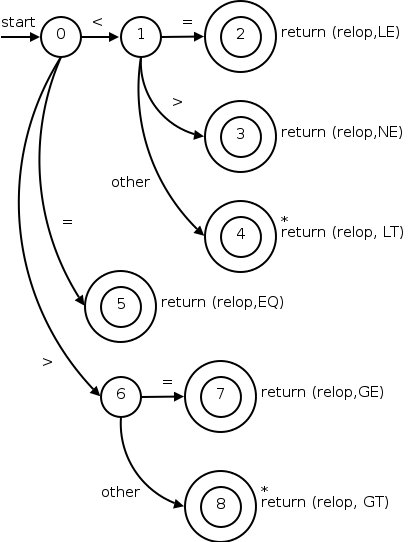
3.4.1: Transition Diagrams
A transition diagram is similar to a flowchart for (a part of) the lexer.
We draw one for each possible token.
It shows the decisions that must be made based on the input seen.
The two main components are circles representing states (think of
them as decision points of the lexer) and arrows
representing edges (think of them as the decisions made).
The transition diagram (3.13) for relop is shown on the right.
- The double circles represent accepting or final
states at which point a lexeme has been found.
There is often an action to be done (e.g., returning the token),
which is written to the right of the double circle.
- If we have moved one (or more) characters
too far
in
finding the token, one (or more) stars are drawn.
- An imaginary start state exists and has an arrow coming from it
to indicate where to begin the process.
It is fairly clear how to write code corresponding to this diagram.
You look at the first character, if it is <, you look at the next
character.
If that character is =, you return (relop,LE) to the parser.
If instead that character is >, you return (relop,NE).
If it is another character, return (relop,LT) and adjust the input
buffer so that you will read this character again since you have not
used it for the current lexeme.
If the first character was =, you return (relop,EQ).
3.4.2: Recognition of Reserved Words and Identifiers
The next transition diagram corresponds to the regular definition
given previously.
Note again the star affixed to the final state.
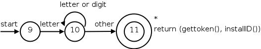
Two questions remain.
- How do we distinguish between identifiers and keywords such
as
then
, which also match the pattern in the transition diagram?
- What is (gettoken(), installID())?
We will continue to assume
that the keywords are reserved, i.e., may not be used as
identifiers.
(What if this is not the case—as in Pl/I, which had no
reserved words?
Then the lexer does not distinguish between keywords and identifiers
and the parser must.)
We will use the method mentioned last chapter and have the keywords
installed into the identifier table prior to any invocation of the
lexer.
The table entry will indicate that the entry is a keyword.
installID() checks if the lexeme is already in the table.
If it is not present, the lexeme is installed as an id token.
In either case a pointer to the entry is returned.
gettoken() examines the lexeme and returns the token name, either id
or a name corresponding to a reserved keyword.
The text also gives another method to distinguish between
identifiers and keywords.
3.4.3: Completion of the Running Example
So far we have transition diagrams for identifiers (this diagram
also handles keywords) and the relational operators.
What remains are whitespace, and numbers, which are respectively the
simplest and most complicated diagrams seen so far.
Recognizing Whitespace
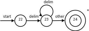
The diagram itself is quite simple reflecting the simplicity of the
corresponding regular expression.
- The
delim
in the diagram represents any of the whitespace
characters, say space, tab, and newline.
- The final star is there because we needed to find a
non-whitespace character in order to know when the whitespace ends
and this character begins the next token.
- There is no action performed at the accepting state.
Indeed the lexer does not return to the parser, but starts
again from its beginning as it still must find the next token.
Recognizing Numbers
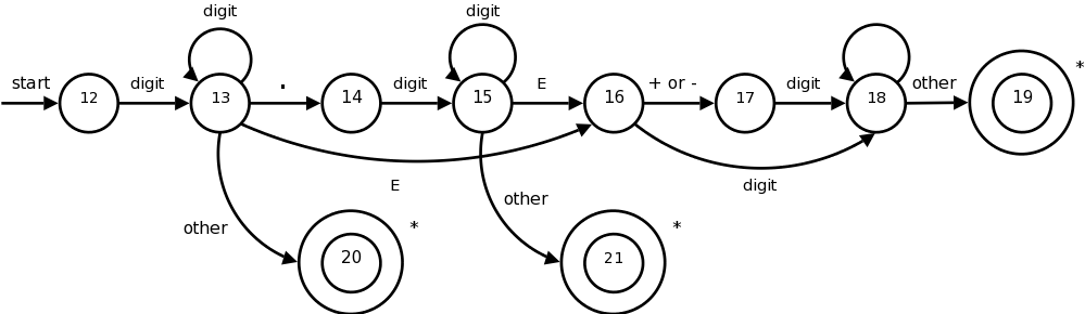
This certainly looks formidable, but it is not that bad;
it follows from the regular expression.
In class go over the regular expression and show the corresponding
parts in the diagram.
When an accepting states is reached, action is required but is not
shown on the diagram.
Just as identifiers are stored in a identifier table and a pointer is
returned, there is a corresponding number table in which numbers are
stored.
These numbers are needed when code is generated.
Depending on the source language, we may wish to indicate in the
table whether this is a real or integer.
A similar, but more complicated, transition diagram could be
produced if the language permitted complex numbers as well.
Homework: 1 (only the ones done before).
3.4.4: Architecture of a Transition-Diagram-Based Lexical Analyzer
The idea is that we write a piece of code for each decision
diagram.
I will show the one for relational operations below.
This piece of code contains a case for each state, which typically
reads a character and then goes to the next case depending on the
character read.
The numbers in the circles are the names of the cases.
Accepting states often need to take some action and return to the
parser.
Many of these accepting states (the ones with stars) need
to restore one character of input.
This is called retract() in the code.
What should the code for a particular diagram do if at one state
the character read is not one of those for which a next state has
been defined?
That is, what if the character read is not the label of any of the
outgoing arcs?
This means that we have failed to find the token corresponding to
this diagram.
The code calls fail().
This is not an error case.
It simply means that the current input does not match this
particular token.
So we need to go to the code section for another diagram after
restoring the input pointer so that we start the next diagram at the
point where this failing diagram started.
If we have tried all the diagram, then we have a real failure and
need to print an error message and perhaps try to repair the input.
Note that the order the diagrams are tried is important.
If the input matches more than one token, the first one tried will
be chosen.
    TOKEN getRelop()                        // TOKEN has two components
      TOKEN retToken = new(RELOP);          // First component set here
      while (true)
         switch(state)
           case 0: c = nextChar();
                   if (c == '<')      state = 1;
                   else if (c == '=') state = 5;
                   else if (c == '>') state = 6;
                   else fail();
                   break;
           case 1: ...
           ...
           case 8: retract();  // an accepting state with a star
                   retToken.attribute = GT;  // second component
                   return(retToken);
Alternate Methods
The book gives two other methods for combining the multiple
transition-diagrams (in addition to the one above).
- Unlike the method above, which tries the diagrams one at a time,
the first new method tries them in parallel.
That is, each character read is passed to each diagram (that
hasn't already failed).
Care is needed when one diagram has accepted the input, but others
still haven't failed and may accept a longer prefix of the input.
-
The final possibility discussed, which appears to be promising, is
to combine all the diagrams into one.
That is easy for the example we have been considering because all
the diagrams begin with different characters being matched.
Hence we just have one large start with multiple outgoing edges.
It is more difficult when there is a character that can begin more
than one diagram.
3.5: The Lexical Analyzer Generator Lex
We are skipping 3.5 because
- We will be writing our lexer from scratch.
- What is here is not enough to learn how to use lex/flex.
- If you are interested in learning how to use them you need to
read (at least) the manual.
The newer version is called flex, the f stands for fast.
I checked and both lex and flex are on the cs machines.
I will use the name lex for both.
Lex is itself a compiler that is used in the construction of other
compilers (its output is the lexer for the other compiler).
The lex language, i.e, the input language of the lex compiler,
is described in the few sections.
The compiler writer uses the lex language to specify the tokens of
their language as well as the actions to take at each state.
3.5.1: Use of Lex
Let us pretend I am writing a compiler for a language called pink.
I produce a file, call it lex.l, that describes pink in a manner
shown below.
I then run the lex compiler (a normal program), giving it lex.l as
input.
The lex compiler output is always a file called lex.yy.c, a program
written in C.
One of the procedures in lex.yy.c (call it pinkLex()) is the lexer
itself, which reads a character input stream and produces a
sequence of tokens.
pinkLex() also sets a global value yylval that is shared with the
parser.
I then compile lex.yy.c together with a the parser (typically the
output of lex's cousin yacc, a parser generator) to produce say
pinkfront, which is an executable program that is the front end for
my pink compiler.
3.5.2: Structure of Lex Programs
The general form of a lex program like lex.l is
      declarations
      %%
      translation rules
      %%
      auxiliary functions
The lex program for the example we have been working with follows
(it is typed in straight from the book).
      %{
          /* definitions of manifest constants
             LT, LE, EQ, NE, GT, GE,
             IF, THEN, ELSE, ID, NUMBER, RELOP */
      %}

      /* regular definitions */
      delim     [ \t\n]
      ws        {delim}*
      letter    [A-Za-z]
      digit     [0-9]
      id        {letter}({letter}{digit})*
      number    {digit}+(\.{digit}+)?(E[+-]?{digit}+)?

      %%

      {ws}      {/* no action and no return */}
      if        {return(IF);}
      then      {return(THEN);}
      else      {return(ELSE);}
      {id}      {yylval = (int) installID(); return(ID);}
      {number}  {yylval = (int) installNum(); return(NUMBER);}
      "<"       {yylval = LT; return(RELOP);}
      "<="      {yylval = LE; return(RELOP);}
      "="       {yylval = EQ; return(RELOP);}
      "<>"      {yylval = NE; return(RELOP);}
      ">"       {yylval = GT; return(RELOP);}
      ">="      {yylval = GE; return(RELOP);}

      %%

      int installID() {/* function to install the lexeme, whose first
	                  character is pointed to by yytext, and whose
                          length is yyleng, into the symbol table and
                          return a pointer thereto */
      }

      int installNum() {/* similar to installID, but puts numerical
	                   constants into a separate table */
The first, declaration, section includes variables and constants as
well as the all-important regular definitions that define the
building blocks of the target language, i.e., the language that the
generated lexer will analyze.
The next, translation rules, section gives the patterns of the
lexemes that the lexer will recognize and the actions to be
performed upon recognition.
Normally, these actions include returning a token name to the parser
and often returning other information about the token via the shared
variable yylval.
If a return is not specified the lexer continues executing and
finds the next lexeme present.
Comments on the Lex Program
Anything between %{ and %} is not processed by lex, but instead is
copied directly to lex.yy.c.
So we could have had statements like
      #define LT 12
      #define LE 13
The regular definitions are mostly self explanatory.
When a definition is later used it is surrounded by {}.
A backslash \ is used when a special symbol like * or . is to be
used to stand for itself, e.g. if we wanted to match a literal star
in the input for multiplication.
Each rule is fairly clear: when a lexeme is matched by the left,
pattern, part of the rule, the right, action, part is executed.
Note that the value returned is the name (an integer) of the
corresponding token.
For simple tokens like the one named IF, which correspond to only
one lexeme, no further data need be sent to the parser.
There are several relational operators so a specification of which
lexeme matched RELOP is saved in yylval.
For id's and numbers's, the lexeme is stored in a table by the
install functions and a pointer to the entry is placed in yylval for
future use.
Everything in the auxiliary function section is copied directly to
lex.yy.c.
Unlike declarations enclosed in %{ %}, however, auxiliary functions
may be used in the actions
3.5.3: Conflict Resolution in Lex
- Match the longest possible prefix of the input.
- If this prefix matches multiple patterns, choose the first.
The first rule makes = one instead of two lexemes.
The second rule makes if
a keyword and not an id.
3.5.3a: Anger Management in Lex
Sorry.
3.5.4: The Lookahead Operator
Sometimes a sequence of characters is only considered a certain
lexeme if the sequence is followed by specified other sequences.
Here is a classic example.
Fortran, PL/I, and some other languages do not have reserved words.
In Fortran
IF(X)=3
is a legal assignment statement and the IF is an identifier.
However,
IF(X.LT.Y)X=Y
is an if/then statement and IF is a keyword.
Sometimes the lack of reserved words makes lexical disambiguation
impossible, however, in this case the slash / operator of lex is
sufficient to distinguish the two cases.
Consider
IF / \(.*\){letter}
This only matches IF when it is followed by a ( some text a ) and a
letter.
The only FORTRAN statements that match this are the if/then shown
above; so we have found a lexeme that matches the if token.
However, the lexeme is just the IF and not the rest of the pattern.
The slash tells lex to put the rest back into the input and match it
for the next and subsequent tokens.
Homework: 1(a-c), 2, 3.
3.6: Finite Automata
The secret weapon used by lex et al to convert (compile
) its
input into a lexer.
Finite automata are like the graphs we saw in transition diagrams
but they simply decide if a sentence (input string) is in the
language (generated by our regular expression).
That is, they are recognizers of the language.
There are two types of finite automata
- Deterministic finite automata (DFA) have for
each state (circle in the diagram) exactly one edge leading out
for each symbol.
So if you know the next symbol and the current state, the next
state is determined.
That is, the
execution
is deterministic; hence the name.
- Nondeterministic finite automata (NFA) are
the other kind.
There are no restrictions on the edges leaving a state: there
can be several with the same symbol as label and some edges can
be labeled with ε.
Thus there can be several possible next states from a given
state and a current
lookahead
symbol.
Surprising Theorem: Both DFAs and NFAs are capable
of recognizing the same languages, the regular languages,
i.e., the languages generated by regular expressions (plus the
automata can recognize the empty language).
What Does This Theorem Mean?
There are certainly NFAs that are not DFAs.
But the language recognized by each such NFA can also be recognized
by at least one DFA.
Why Mention (Confusing) NFAs?
The DFAs that recognizes the same language as an NFA might be
significantly larger than the NFA.
The finite automaton that one constructs naturally from
a regular expression is often an NFA.
3.6.1: Nondeterministic Finite Automata
Here is the formal definition.
A
nondeterministic finite automaton (NFA) consists of
- A finite set of states S.
- An input alphabet Σ not containing
ε.
- A transition function that gives, for each state and
each symbol in Σ ∪ ε, a set of
next states (or successor states).
- An element s0 of S, the start state.
- A subset F of S, the accepting states
(or final states).
An NFA is basically a flow chart like the transition diagrams we
have already seen.
Indeed an NFA (or a DFA, to be formally defined soon) can be
represented by a transition graph whose nodes are states and
whose edges are labeled with elements of Σ ∪ ε.
The differences between a transition graph and our previous
transition diagrams are:
- Possibly multiple edges with the same label leaving a single
state.
- An edge may be labeled with ε.
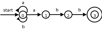
The transition graph to the right is an NFA for
the regular expression (a|b)*abb, which (given the
alphabet {a,b}) represents all words ending in abb.
Consider aababb.
If you choose the wrong
edge for the initial a's you will get
stuck.
But an NFA accepts a word if any path (beginning at the start
state and using the symbols in
the word in order) ends at an accepting state.
It essentially tries all such paths at once and accepts if any end
at an accepting state.
This means in addition that, if some paths uses all the input and
end in a non-accepting state, but at least one path uses all the
input (doesn't get stuck) and ends in an accepting state, the input
is accepted.
Remark: Patterns like (a|b)*abb are useful regular
expressions!
If the alphabet is ascii, consider *.java.
Homework: 3, 4.
3.6.2: Transition Tables
| State | a | b | ε |
|---|
| 0 | {0,1} | {0} | φ |
| 1 | φ | {2} | φ |
| 2 | φ | {3} | φ |
There is an equivalent way to represent an NFA, namely a table
giving, for each state s and input symbol x (and ε), the
set of successor states x leads to from s.
The empty set φ is used when there is no edge labeled x
emanating from s.
The table on the right corresponds to the transition graph above.
The downside of these tables is their size, especially if most of
the entries are φ since those entries would not take any space
in a transition graph.
Homework: 5.
3.6.3: Acceptance of Input Strings by Automata
An NFA accepts a string if the symbols
of the string specify a path from the start to an accepting state.
Note that these symbols may specify several paths, some of
which lead to accepting states and some that don't.
In such a case the NFA does accept the string; one successful path
is enough.
Also note that if an edge is labeled ε, then it can be
taken for free
.
For the transition graph above any string can just sit at state 0
since every possible symbol (namely a or b) can go from state 0 back
to state 0.
So every string can lead to a non-accepting state, but that is not
important since, if just one path with that string leads to an
accepting state, the NFA accepts the string.
The language defined by an NFA or the
language accepted by an NFA is the set of strings
(a.k.a. words) accepted by the NFA.
So the NFA in the diagram above accepts the same language as the
regular expression (a|b)*abb.
If A is an automaton (NFA or DFA) we use L(A) for the language
accepted by A.
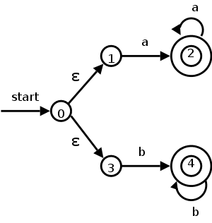
The diagram on the right illustrates an NFA accepting the language
L(aa*|bb*).
The path
0 → 3 → 4 → 4 → 4 → 4
shows that bbbb is accepted by the NFA.
Note how the ε that labels the edge 0 → 3 does not
appear in the string bbbb since ε is the empty string.
3.6.4: Deterministic Finite Automata
There is something weird about an NFA if viewed as a model of
computation.
How is a computer of any realistic construction able to check out
all the (possibly infinite number of) paths to determine if any
terminate at an accepting state?
We now consider a much more realistic model, a DFA.
Definition: A
deterministic finite automata or DFA is a special
case of an NFA having the restrictions
- No edge is labeled with ε
- For any state s and symbol a, there is
exactly one edge leaving s with label a.
(If no edge is shown with label a, there is an implied edge
leading to a node labeled fail.)
This is realistic.
We are at a state and examine the next character in the string,
depending on the character we go to exactly one new state.
Looks like a switch statement to me.
Minor point: when we write a transition table for a DFA, the
entries are elements not sets so there are no {} present.
Simulating a DFA
Indeed a DFA is so reasonable there is an obvious algorithm for
simulating it (i.e., reading a string and deciding whether or not it
is in the language accepted by the DFA).
We present it now.
    s := s0;   // start state.
    c := nextChar();      // a priming read
    while (c /= eof) {
      s := move(s,c);
      c := nextChar();
    }
    if (s is in F, the set of accepting states) return yes
    else return no
3.7: From Regular Expressions to Automata
3.7.0: Not Losing Site of the Forest Due to the Trees
This is not from the book.
Do not forget the goal of the chapter is to understand lexical
analysis.
(Languages generated by) regular expressions are the key to this task,
since we use them to specify tokens.
So we want to recognize (languages generated by) regular expressions.
We are going to see two methods.
- Convert the regular expression to an NFA and simulate the NFA.
- Convert the regular expression to an NFA, convert the NFA to a
DFA, and simulate the DFA.
So we need to learn 4 techniques.
- Convert a regular expression to an NFA
- Simulate an NFA
- Convert an NFA to a DFA
- Simulate a DFA.
The list I just gave is in the order the algorithms would be
applied—but you would use either 2 or (3 and 4).
However, we will follow the order in the book, which is exactly the
reverse.
Indeed, we just did item #4 and will now do #3.
3.7.1: Converting an NFA to a DFA
The book gives a detailed proof; I am just trying to motivate the
ideas.
Let N be an NFA, we construct D, a DFA that accepts the same strings
as does N.
Call a state of N an N-state, and call a state of D a D-state.
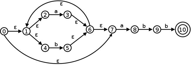
The idea is that a D-state corresponds to a set of N-states and
hence the procedure we are describing is called the
subset algorithm.
Specifically for each string X of symbols we consider all the
N-states that can result when N processes X.
This set of N-states is a D-state.
Let us consider the transition graph on the right, which is an NFA
that accepts strings satisfying the regular expression
(a|b)*abb.
The alphabet is {a,b}.
The start state of D is the set of N-states that can result when N
processes the empty string ε.
This is called the ε-closure of the start state
s0 of N, and consists of those N-states that can be
reached from s0 by following edges labeled with ε.
Specifically it is the set {0,1,2,4,7} of N-states.
We call this state D0 and enter it in the transition
table we are building for D on the right.
| NFA states | DFA state | a | b |
|---|
| {0,1,2,4,7} | D0 | D1 | D2 |
| {1,2,3,4,6,7,8} | D1 | D1 | D3 |
| {1,2,4,5,6,7} | D2 | D1 | D2 |
| {1,2,4,5,6,7,9} | D3 | D1 | D4 |
| {1,2,4,5,6,7,10} | D4 | D1 | D2 |
Next we want the a-successor of D0, i.e., the D-state
that occurs when we start at D0 and move along an edge
labeled a.
We call this successor D1.
Since D0 consists of the N-states corresponding to
ε, D1 is the N-states corresponding
to εa
=a
.
We compute the a-successor of all the N-states in D0 and
then form the ε-closure.
Next we compute the b-successor of D0 the same way and
call it D2.
We continue forming a- and b-successors of all the D-states until
no new D-states result (there are only a finite number of subsets of
all the N-states so this process does indeed stop).
This gives the table on the right.
D4 is the only D-accepting state as it is the only
D-state containing the (only) N-accepting state 10.
Theoretically, this algorithm is awful since for a set
with k elements, there are 2k subsets.
Fortunately, normally only a small fraction of the possible subsets
occur in practice.
For example, the NFA we just did had 11 states so there are 2048
possible subsets, only 5 of which occurred in the DFA we
constructed.
Homework: 1.
3.7.2: Simulating an NFA
Instead of producing the DFA, we can run the subset algorithm as a
simulation itself.
This is item #2 in my list of techniques
S = ε-closure(s0);
c = nextChar();
while ( c != eof ) {
S = ε-closure(move(S,c));
c = nextChar();
}
if ( S ∩ F != φ ) return yes
; // F is accepting states
else return no
;
Homework: 2.
3.7.3: Efficiency of NFA Simulation
Slick implementation.
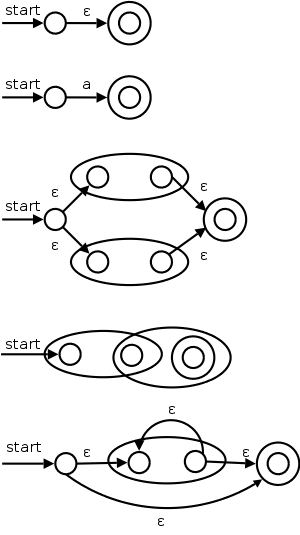
3.7.4: Constructing an NFA from a Regular Expression
I give a pictorial proof by induction.
This is item #1 from my list of techniques.
- The base cases are the empty regular expression and the regular
expression consisting of a single symbol a in the alphabet.
- The inductive cases are.
- s | t for s and t regular expressions
- st for s and t regular expressions
- s*
- (s), which is trivial since the nfa for s also works for
(s).
- We have so few cases because regular expressions (w/o
extensions) are sufficient.
That is, once we can construct arbitrary REs, we can also
construct the extended REs and the regular definitions since
both of these can be expressed as REs.
The pictures on the right illustrate the base and inductive cases.
Remarks:
- The generated NFA has at most twice as many states as there are
operators and operands in the RE.
This is important for studying the complexity of the NFA, which we
will not do.
- The generated NFA has one start and one accepting state.
The accepting state has no outgoing arcs and the start state has
no incoming arcs.
This is important for the pictorial proof we gave since we always
assumed that the constituent NFAs had that property when building
the bigger NFS.
- Note that the diagram for st correctly indicates that the final
state of s and the initial state of t are merged.
This is one use of the previous remark that there is only one
start state and one final state.
- Except for the accepting state, each state of the generated NFA
has either one outgoing arc labeled with a symbol or two outgoing
arcs labeled with ε.
Do the NFA for (a|b)*abb and see that we get the same
diagram that we had before.
Do the steps in the normal leftmost, innermost order (or
draw a normal parse tree and follow it).
Homework: 3 a,b,c
3.7.5: Efficiency of String-Processing Algorithms
3.8: Design of a Lexical-Analyzer Generator
How lexer-generators like Lex work.
Since your lab2 is to produce a lexer, this is also a section on how
you should solve lab2.
Start Lecture #5
3.8.1: The structure of the generated analyzer
We have seen simulators for DFAs and NFAs.
The remaining large question is how is the lex input converted into
one of these automatons.
Also
- Lex permits functions to be passed through to the yy.lex.c file.
This is fairly straightforward to implement, but
is not part of lab2.
- Lex also supports actions that are to be invoked by the
simulator when a match occurs.
This is also fairly straight forward, but again
is not part of lab2.
- The lookahead operator is not so simple in the general case
and is discussed briefly below, but again is
not part of lab2.
In this section we will use transition graphs.
Of course lexer-generators do not draw pictures; instead they use the
equivalent transition tables.
Recall that the regular definitions in Lex are mere conveniences
that can easily be converted to REs and hence we need only convert
REs into an FSA.
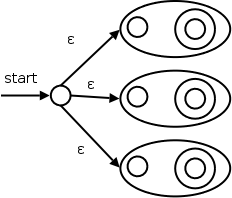
We already know how to convert a single RE into an NFA.
But lex input will contain (and lab 2 does contain) several REs
since it wishes to recognize several different tokens.
The solution is to
- Produce an NFA for each RE.
- Introduce a new start state.
- Introduce an ε transition from the new start state to
the start of each NFA constructed in step 1.
- When one of the NFAs reaches one of the accepting states, the
simulation does NOT stop.
See below for an explanation.
The result is shown to the right.
Label each of the accepting states (for all NFAs constructed in
step 1) with the actions specified in the lex program for the
corresponding pattern.
3.8.2: Pattern Matching Based on NFAs
We use the algorithm for simulating NFAs presented in 3.7.2.
The simulator starts reading characters and calculates the set of
states it is at.
| Pattern | Action to perform |
|---|
| a | Action1 |
| abb | Action2 |
| a*bb* | Action3 |
At some point the input character does not lead to any state or we
have reached the eof.
Since we wish to find the longest lexeme matching the
pattern we proceed backwards from the current point (where there was
no state) until we reach an accepting state (i.e., the set of
N-states contains an accepting N-state).
Each accepting N-state corresponds to a matched pattern.
The lex rule is that if a lexeme matches multiple patterns we choose
the pattern listed first in the lex-program.
I don't believe this rule will be needed in lab 2 since I can't
think of a case where two different patterns will match the same
(longest) lexeme.
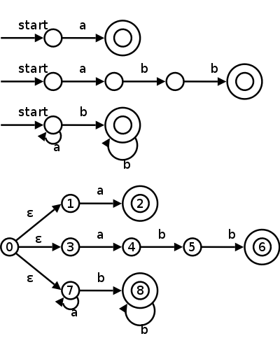
Example
Consider the example just above with three patterns and their
associated actions and consider processing the input aaba.
- We begin by constructing the three NFAs.
To save space, the third NFA is not the one that would be
constructed by our algorithm, but is an equivalent smaller one.
For example, some unnecessary ε-transitions have been
eliminated.
If one views the lex executable as a compiler transforming lex
source into NFAs, this would be considered an
optimization
.
- We introduce a new start state and ε-transitions as in
the previous section.
- We start at the ε-closure of the start state, which is
{0,1,3,7}.
- The first a (remember the input is aaba) takes us to {2,4,7}.
This includes an accepting state and indeed we have matched the
first patten.
However, we do not stop since we may find a longer match.
- The next a takes us to {7}.
- The b takes us to {8}.
- The next a fails since there are no a-transitions out of state
8.
So we must back up to before trying the last a.
- We are back in {8} and ask if one of these N-states (I know there
is only one, but there could be more) is an accepting state.
- Indeed state 8 is accepting for third pattern.
If there were more than one accepting state in the list, we would
choose the one in the earliest listed pattern.
- Action3 would now be performed.
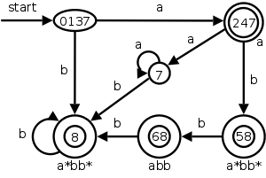
3.8.3: DFA's for Lexical Analyzers
We could also convert the NFA to a DFA and simulate that.
The resulting DFA is on the right.
Note that it shows the same D-states (i.e., sets of N-states) we saw
in the previous section, plus some other D-states that arise from
inputs other than aaba.
We label the accepting states with the pattern matched.
If multiple patterns are matched (because the accepting D-state
contains multiple accepting N-states), we use the first
pattern listed (assuming we are using lex conventions).
For example, the middle D-state on the bottom row contains two
accepting N-states, 6 and 8.
Since the RE for 6 was listed first, it appears below the state.
Consider processing the string aa
.
Show how you get two tokens.
Technical point.
For a DFA, there must be a outgoing edge from each D-state for each
possible character.
In the diagram, when there is no NFA state possible, we do not show
the edge.
Technically we should show these edges, all of which lead to the
same D-state, called the dead state, and corresponds to the empty
subset of N-states.
Remark: A pure DFA or NFA simply accepts or
rejects a single string.
In the context of lexers, that would mean accepting or rejecting a
single lexeme.
But a lexer isn't given a single lexeme to process, it is given a
program consisting of many lexemes.
That is why we have the complication of backtracking after getting
stuck; a pure NFA/DFA would just say reject if the next character
did not correspond to an outgoing arc.
Alternatives for Implementing Lab 2
There are trade-offs depending on how much you want to do by hand
and how much you want to program.
At the extreme you could write a program that reads in the regular
expression for the tokens and produces a lexer, i.e., you could
write a lexical-analyzer-generator.
I very much advise against this, especially since
the first part of the lab requires you to draw the transition
diagrams anyway.
The two reasonable alternatives are.
- By hand, convert the NFA to a DFA and then write your lexer
based on this DFA, simulating its actions for input strings.
- Write your program based on the NFA.
3.8.4: Implementing the Lookahead Operator
This has some tricky points; we are basically skipping it.
This lookahead operator is for when you must look further down the
input but the extra characters matched are not part of the lexeme.
We write the pattern r1/r2.
In the NFA we match r1 then treat the / as an ε and then
match s1.
It would be fairly easy to describe the situation when the NFA has
only one ε-transition at the state where r1 is matched.
But it is tricky when there are more than one such transition.
3.9: Optimization of DFA-Based Pattern Matchers
3.9.1: Important States of an NFA
3.9.2: Functions Computed form the Syntax Tree
3.9.3: Computing nullable, firstpos, and lastpos
3.9.4: Computing followpos
Remark: Lab 2 assigned.
Part 1 (no programming) due in one week; the remainder is due in 2
weeks (i.e, one week after part 1).
Chapter 4: Syntax Analysis
Homework: Read Chapter 4.
4.1: Introduction
4.1.1: The role of the parser
As we saw in the previous chapter the parser calls the lexer to
obtain the next token.
Conceptually, the parser accepts a sequence of tokens and produces
a parse tree.
In practice this might not occur.
- The source program might have errors.
Shamefully, we will do very little error handling.
- Instead of explicitly constructing the parse tree, the actions
that the downstream components of the front end would do on the
tree can be integrated with the parser and done incrementally on
components of the tree.
We will see examples of this, but your lab number 3 will produce
a parse tree.
Your lab number 4 will process this parse tree and do the
actions.
- Real compilers produce (abstract) syntax trees not parse trees
(concrete syntax trees).
We don't do this for the pedagogical reasons given previously.
There are three classes for grammar-based parsers.
- universal
- top-down
- bottom-up
The universal parsers are not used in practice as they are
inefficient; we will not discuss them.
As expected, top-down parsers start from the root of the tree and
proceed downward; whereas, bottom-up parsers start from the leaves
and proceed upward.
The commonly used top-down and bottom parsers are not
universal.
That is, there are context-free grammars that cannot be used with
them.
The LL (top down) and LR (bottom-up) parsers are important in practice.
Hand written parsers are often LL.
Specifically, the predictive parsers we looked at in chapter two are
for LL grammars.
The LR grammars form a larger class.
Parsers for this class are usually constructed with the aid of
automatic tools.
4.1.2: Representative Grammars
Expressions with + and *
    E → E + T | T
    T → T * F | F
    F → ( E ) | id
This takes care of precedence, but as we saw before, gives
predictive parsing trouble since it is left-recursive.
So we used the following non-left-recursive grammar that generates
the same language.
    E  → T E'
    E' → + T E' | ε
    T  → F T'
    T' → * F T' | ε
    F  → ( E ) | id
The following ambiguous grammar will be used for illustration, but
in general we try to avoid ambiguity.
E → E + E | E * E | ( E ) | id
This grammar does not enforce precedence and it does not specify
left vs right associativity.
For example, id + id + id and id + id * id each have two parse
trees.
4.1.3: Syntax Error Handling
There are different levels
of errors.
- Lexical errors: For example, spelling.
- Syntactic errors: For example missing ; .
- Semantic errors: For example wrong number of array indexes.
- Logical errors: For example
off by one
usage of <
instead of <=.
4.1.4: Error-Recovery Strategies
The goals are clear, but difficult.
- Report errors clearly and accurately.
One difficulty is that one error can mask another and can cause
correct code to look faulty.
- Recover quickly enough to not miss other errors.
- Add minimal overhead.
Trivial Approach: No Recovery
Print an error message when parsing cannot continue and then
terminate parsing.
Panic-Mode Recovery
The first level improvement.
The parser discards input until it encounters a
synchronizing token.
These tokens are chosen so that the parser can make a fresh
beginning.
Good examples for C/Java are ; and }.
Phrase-Level Recovery
Locally replace some prefix of the remaining input by some string.
Simple cases are exchanging ; with , and = with ==.
Difficulties occur when the real error occurred long before an error
was detected.
Error Productions
Include productions for common errors
.
Global Correction
Change the input I to the closest
correct input I' and
produce the parse tree for I'.
4.2: Context-Free Grammars
4.2.1: Formal Definition
Definition: A Context-Free Grammar
consists of
- Terminals: The basic components found by the lexer.
They are sometimes called token names, i.e., the first component
of the token as produced by the lexer.
- Nonterminals: Syntactic variables that help define the syntactic
structure of the language.
- Start Symbol: A nonterminal that forms the root of the parse tree.
- Productions:
- Head or left (hand) side or LHS.
For context-free grammars, which are our only
interest, the LHS must consist of just a single nonterminal.
- →
- Body or right (hand) side or RHS.
A string of terminals and nonterminals.
4.2.2: Notational Conventions
I am not as formal as the book.
In particular, I don't use italics.
Nonetheless I do (try to) use some of the conventions, in particular
the ones below.
Please correct me if I violate them.
- Uppercase letters early in the alphabet like A, B, and C are
use to represent nonterminals.
Also S is often used as the start symbol, but remember that if
no explicit start symbol is given for a grammar, than the LHS of
the first production is the start symbol.
- Lowercase letters early in the alphabet are used to represent
terminals.
- Uppercase letters late in the alphabet are used to represent a
single grammar symbol, i.e., either a single terminal or a
single nonterminal.
- Lowercase letters late in the alphabet represent are used to
represent a (possibly empty) string of terminals.
- Lowercase Greek letters are used to represent a (possibly
empty) string of grammar symbols.
I never use ε for this purpose since ε always
represents the empty string.
- So A → α would be a generic production in a
context-free grammar.
- X → α and β → α include illegal
productions for a context-free grammar.
As I have mentioned before, when the entire grammar is written, no
conventions are needed to tell the nonterminals, terminals, and
start symbol.
The nonterminals are the LHSs, the terminals are everything else on
the RHS, and the start symbol is the LHS of the first production.
The the notational conventions are used when you just give a few
productions not a full grammar.
4.2.3: Derivations
This is basically just notational convenience, but important
nonetheless.
Assume we have a production A → α.
We would then say that A derives α and write
A ⇒ α
We generalize this.
If, in addition, β and γ are strings (each may contain
terminals and/or nonterminals), we say that
βAγ derives βαγ and write
βAγ ⇒ βαγ
We say that βAγ derives βαγ
in one step.
We generalize further.
If α derives β and β derives γ, we say α
derives γ and write
α ⇒* γ.
The notation used is ⇒ with a * over it (I don't see it in
html).
This should be read derives in zero or more steps
.
Formally,
- α ⇒* α, for any string α.
- If α ⇒* β and β ⇒ γ,
then α ⇒* γ.
Informally, α ⇒* β means you can get from α to
β, and α ⇒ β means you can get from α to
β in one step.
Definition: If S is the start symbol and
S⇒*α, we say α is a
sentential form of the grammar.
A sentential form may contain nonterminals and terminals.
Definition: A sentential form containing only
terminals is called a sentence of the grammar.
Definition: The language
generated by a grammar G, written L(G), is the set of
these sentences.
Definition: A language generated by a
(context-free) grammar is called a context free
language.
Definition: Two grammars generating the same
language are called equivalent.
Examples: Recall the ambiguous grammar above
E → E + E | E * E | ( E ) | id
We see that id + id is a sentence.
Indeed it can be derived in two ways from the start symbol E.
    E ⇒ E + E ⇒ id + E ⇒ id + id
    E ⇒ E + E ⇒ E + id ⇒ id + id
(Since both derivations give the same parse tree, this does not
show the grammar is ambiguous.
You should be able to find a sentence—without looking back in
the notes—that has two different parse trees.)
In the first derivation shown just above, each step replaced the
leftmost nonterminal by the body of a production having the
nonterminal as head.
This is called a leftmost derivation.
Similarly the second derivation, in which each step replaced the
rightmost nonterminal, is called a rightmost derivation.
Sometimes the latter are called canonical derivations,
but we won't do so.
When one wishes to emphasize that a (one step) derivation is leftmost
they write an lm under the ⇒.
To emphasize that a (general) derivation is leftmost, one writes an lm
under the ⇒*.
Similarly one writes rm to indicate that a derivation is rightmost.
I won't do this in the notes but will on the board.
Definition: If x can be derived using a leftmost
derivation, we call x a left-sentential form.
Similarly for a right-sentential form.
Homework: 1(ab), 2(ab).
4.2.4: Parse Trees and Derivations
The leaves of a parse tree (or of any other tree), when read left
to right, are called the frontier of the tree.
For a parse tree we also call them the yield of the tree.
If you are given a derivation starting with a single nonterminal,
A ⇒ α1 ⇒ α2
... ⇒ αn
it is easy to write a parse tree with A as the root and
αn as the leaves.
Just do what (the production contained in) each step of the
derivation says.
The LHS of each production is a nonterminal in the frontier of the
current tree so replace it with the RHS to get the next tree.
Do this for both the leftmost and rightmost derivations of id+id
above.
So there can be many derivations that wind up with the same final
tree.
But for any parse tree there is a unique leftmost derivation
producing that tree (always choose the leftmost unmarked
nonterminal to be the LHS, mark it, and write the production with
this LHS and the children as the RHS).
Similarly, there is a unique rightmost derivation that produces the
tree.
There may be others as well (e.g., sometime choose the leftmost
unmarked nonterminal to expand and other times choose the
rightmost; or choose a middle
unmarked nonterminal).
Homework: 1c
4.2.5: Ambiguity
Recall that an ambiguous grammar is one for which there is more
than one parse tree for a single sentence.
Since each parse tree corresponds to exactly one leftmost
derivation, a grammar is ambiguous if and only if it permits more
than one leftmost derivation of a given sentence.
Similarly, a grammar is ambiguous if and only if it permits more
than one rightmost of a given sentence.
We know that the grammar
E → E + E | E * E | ( E ) | id
is ambiguous.
For example, there are two parse trees for
id + id * id
So there must me at least two leftmost derivations.
Here they are
    E ⇒ E + E          E ⇒ E * E
      ⇒ id + E           ⇒ E + E * E
      ⇒ id + E * E       ⇒ id + E * E
      ⇒ id + id * E      ⇒ id + id * E
      ⇒ id + id * id     ⇒ id + id * id
As we stated before we prefer unambiguous grammars.
Failing that, we want disambiguation rules, as are often given for
the dangling else in the C language.
4.2.6: Verification
4.2.7: Context-Free Grammars Versus Regular Expressions
Alternatively context-free languages vs regular languages.
Given an RE, we learned in Chapter 3 how to construct an NFA
accepting the same strings.
Now we show that, given an NFA, we can construct an RE accepting
the same string
- Define a nonterminal Ai for each state i.
- For a transition from Ai to Aj
on input a (or ε), add a production
Ai → aAj
(or Ai → Aj).
- If i is accepting, add Ai → ε
- If i is start, make Ai start.
If you trace an NFA accepting a sentence, it just corresponds to
the constructed grammar deriving the same sentence.
Similarly, follow a derivation and notice that at any point prior to
acceptance there is only one nonterminal; this nonterminal
gives the state in the NFA corresponding to this point in the
derivation.
The book starts with (a|b)*abb and then uses the short NFA on the
left below.
Recall that the NFA generated by our construction is the longer one
on the right.
The book gives the simple grammar for the short diagram.
Let's be ambitious and try the long diagram
    A0 → A1 | A7
    A1 → A2 | A4
    A2 → a A3
    A3 → A6
    A4 → b A5
    A5 → A6
    A6 → A1 | A7
    A7 → a A8
    A8 → b A9
    A9 → b A10
    A10 → ε
Now trace a path in the NFA beginning at the start state and see
that it is just a derivation.
That is the string corresponding to that path is a sentential form.
The same is true in reverse (derivation gives path).
The key is that at every stage you have at only one nonterminal.
Then notice that when you get to an accepting state, you have no
nonterminals so accepting a string in the NFA shows it is a
sentence in the language
Grammars, but not Regular Expressions, Can Count
The grammar
A → c A b | ε
generates all strings of the form cnbn, where
there are the same number of c's and b's.
In a sense the grammar has counted.
No RE can generate this language.
A proof is in the book.
The idea is that you need a infinite number of states to represent
the number of c's you have seen so that you can ensure that you see
the same number of b's.
But a RE is equivalent to a DFA (or NFA) and the F stands for
finite.
4.3: Writing a Grammar
4.3.1: Lexical vs Syntactic Analysis
Why have a separate lexer and parser?
Since the lexer deals with REs / Regular Languages and the parser
deals with the more powerful Context Free Grammars (CFGs) / Context
Free Languages (CFLs), everything a lexer can do, a parser could do
as well.
The reasons for separating the lexer and parser are from software
engineering considerations.
- REs are easier than CFGs to understand.
- More efficient algorithms/tools exist for automating the
RE-based lexer than for the CFG-based parser.
- Only the lexer need deal with the external environment.
4.3.2: Eliminating Ambiguity
Recall the ambiguous grammar with the notorious
dangling else
problem.
      stmt → if expr then stmt
      | if expr then stmt else stmt
      | other
This has two leftmost derivations for
if E1 then if E2 then S1 else S2
Do these on the board.
They differ in the beginning.
In this case we can find a non-ambiguous, equivalent grammar.
        stmt → matched-stmt | open-stmt
matched-stmt → if expr then matched-stmt else matched-stmt
	     | other
   open-stmt → if expr then stmt
	     | if expr then matched-stmt else open-stmt
On the board find the unique parse tree for the problem sentence
and from that the unique leftmost derivation.
Remark:
There are three areas relevant to the above example.
- Language design.
C vs Ada (end if).
We are not studying this.
- Finding a non-ambiguous grammar for the C if-then-else.
This was not easy.
- Parsing the
dangling else
example with the
non-ambiguous grammar.
We can do this.
End of Remark.
4.3.3: Eliminating Left Recursion
We did special cases in chapter 2.
Now we do it right
(tm).
Previously we did it separately for one production and for two
productions with the same nonterminal on the LHS.
Not surprisingly, this can be done for n such productions (together
with other non-left recursive productions involving the same
nonterminal).
Specifically we start with
A → A α1 | A α2 | ... A αn | β1 | β2 | ... βm
where the α's and β's are strings,
and no β begins with A (otherwise it would be an α).
The equivalent non-left recursive grammar is
    A  → β1 A' | ... | βm A'
    A' → α1 A' | ... | αn A' | ε
The idea is as follows.
Look at the left recursive grammar.
At some point you stop producing more As and have the A (which is always on
the left) become one of the βs.
So the final string starts with a β.
Up to this point all the As became Aα for one of the αs.
So the final string is a β followed by a bunch of αs, which is
exactly what the non-left recursive definition says.
Example: Assume n=m=1, α1 is +
and β1 is *.
So the left recursive grammar is
A → A + | *
and the non-left recursive grammar is
    A  → * A'
    A' → + A' | ε
With the recursive grammar, we have the following derivation.
A ⇒ A + ⇒ A + + ⇒ * + +
With the non-recursive grammar we have
A ⇒ * A' ⇒ * + A' ⇒ * + + A' ⇒ * + +
This procedure removes direct left recursion where a production
with A on the left hand side begins with A on the right.
If you also had direct left recursion with B, you would apply the
procedure twice.
The harder general case is where you permit indirect left
recursion, where, for example one production has A as the LHS and
begins with B on the RHS, and a second production has B on the LHS
and begins with A on the RHS.
Thus in two steps we can turn A into something starting again with
A.
Naturally, this indirection can involve more than 2 nonterminals.
Theorem: All left recursion can be eliminated.
Proof: The book proves this for grammars that have
no ε-productions and no cycles
and has exercises
asking the reader to prove that cycles and ε-productions can
be eliminated.
We will try to avoid these hard cases.
Homework: Eliminate left recursion in the
following grammar for simple postfix expressions.
S → S S + | S S * | a
4.3.4: Left Factoring
If two productions with the same LHS have their RHS beginning with
the same symbol (terminal or nonterminal), then the FIRST sets will
not be disjoint so predictive parsing (chapter 2) will be impossible
and more generally top down parsing (defined later this chapter)
will be more difficult as a longer lookahead will be needed to
decide which production to use.
So convert A → α β1 | α β2 into
   A  → α A'
   A' → β1 | β2
In other words factor out
the α.
Homework: Left factor your answer to the previous
homework.

4.3.5: Non-CFL Constructs
Although our grammars are powerful, they are not all-powerful.
For example, we cannot write a grammar that checks that all
variables are declared before used.
4.4: Top-Down Parsing
We did an example of top down parsing, namely predictive parsing,
in chapter 2.
For top down parsing, we
- Start with the root of the parse tree, which is always the
start symbol of the grammar.
That is, initially the parse tree is just the start symbol.
- Choose a nonterminal in the frontier.
- Choose a production having that nonterminal as LHS.
- Expand the tree by making the RHS the children of the LHS.
- Repeat above until the frontier is all terminals.
- Hope that the frontier equals the input string.
The above has two nondeterministic choices (the nonterminal, and
the production) and requires luck at the end.
Indeed, the procedure will generate the entire language.
So we have to be really lucky to get the input string.
Another problem is that the procedure may not terminate.
4.4.1: Recursive Decent Parsing
Let's reduce the nondeterminism in the above algorithm by
specifying which nonterminal to expand.
Specifically, we do a depth-first (left to right) expansion.
This corresponds to a leftmost derivation.
That is, we expand the leftmost nonterminal in the frontier.
We leave the choice of production nondeterministic.
We also process the terminals in the RHS, checking that they match
the input.
By doing the expansion depth-first, left to right, we ensure that we
encounter the terminals in the order they will appear in the
frontier of the final tree.
Thus if the terminal does not match the corresponding input symbol
now, it never will (since there are no nonterminals to its left) and
the expansion so far will not produce the input string as desired.
Now our algorithm is
- Initially, the tree is the start symbol, the nonterminal we
are currently processing.
- Choose a production having the current nonterminal as LHS and
expand the tree with the RHS, X1 X2 ... Xn.
-
for i = 1 to n
  if Xi is a nonterminal
    process Xi  // recursive call to step 2
  else if Xi (a terminal) matches current input symbol
    advance input to next symbol
  else // trouble Xi doesn't match and never will
Note that the trouble
mentioned at the end of the algorithm
does not signify an erroneous input.
We may simply have chosen the wrong production in step 2.
In a general recursive descent (top-down) parser, we would support
backtracking.
That is, when we hit the trouble, we would go back and choose
another production.
It is possible that no productions work for
this nonterminal, because the wrong choice was made earlier.
In that case we must back up further.
As an example consider the grammar
    S → A a | B b
    A → 1 | 2
    B → 1 | 2
and the input string 1 b
.
On the right we show a movie of a recursive descent parsing of this
string in which we have to backup two steps.
The good news is that we will work with grammars where we can
control the nondeterminism much better.
Recall that for predictive parsing, the use of 1 symbol of lookahead
made the algorithm fully deterministic, without backtracking.
4.4.2: FIRST and FOLLOW
We used FIRST(RHS) when we did predictive parsing.
Now we learn the whole truth about these two sets, which proves to
be quite useful for several parsing techniques (and for error
recovery, but we won't make use of this).
The basic idea is that FIRST(α) tells you what the first
terminal can be when you fully expand the string α and
FOLLOW(A) tells what terminals can immediately
follow the nonterminal A.
Definition: For any string α of grammar
symbols, we define FIRST(α) to be the set of terminals that
occur as the first symbol in a string derived from α.
So, if α⇒*cβ for c a terminal and β a string,
then c is in FIRST(α).
In addition, if α⇒*ε, then ε is in
FIRST(α).
Definition: For any nonterminal A, FOLLOW(A) is the
set of terminals x, that can appear immediately to the right of A in a
sentential form.
Formally, it is the set of terminals c, such that
S⇒*αAcβ.
In addition, if A can be the rightmost symbol in a sentential form
(i.e., if S⇒*αA), the endmarker $ is in FOLLOW(A).
Note that there might have been symbols between A and c during the
derivation, providing they all derived ε and eventually c
immediately follows A.
Unfortunately, the algorithms for computing FIRST and FOLLOW are
not as simple to state as the definition suggests, in large part
caused by ε-productions.
Calculating FIRST
Remember that FIRST(α) is the set of terminals that can
begin a string derived from α.
Since a terminal can derive only itself, FIRST of a terminal is trivial.
FIRST(a) = {a}, for any terminal a
FIRST of a nonterminal is not so easy
- Initialize FIRST(A)=φ for all nonterminals A
- If A → ε is a production, add ε to FIRST(A).
- For each production A → Y1 ... Yn,
- add to FIRST(A) any terminal a satisfying
- a is in FIRST(Yi) and
- ε is in all previous FIRST(Yj).
- add ε to FIRST(A) if ε is in all
FIRST(Yj).
Repeat step 3 until nothing is added.
FIRST of an arbitrary string now follows.
- FIRST of any string X=X1X2...Xn
is initialized to φ.
- add to FIRST(X) any non-ε symbol in
FIRST(Xi) if ε is in all previous
FIRST(Xj).
- add ε to FIRST(X) if ε is in every
FIRST(Xj).
In particular if X is ε, FIRST(X)={ε}.
Calculating FOLLOW
Recall that FOLLOW is defined only for nonterminals A and is the set
of terminals that can immediately follow A in a sentential form (a
string derivable from the start symbol
- Initialize FOLLOW(S)=$ and FOLLOW(A)=φ for all other
nonterminals A.
- For every production A → α B β, add all of
FIRST(β) except ε to FOLLOW(B).
- Apply the following rule until nothing is added to any FOLLOW
set.
For every production ending in B
, i.e. for
A → α B and for
A → α B β,
where FIRST(β) contains ε,
add all of FOLLOW(A) to FOLLOW(B).
Do the FIRST and FOLLOW sets for
    E  → T E'
    E' → + T E' | ε
    T  → F T'
    T' → * F T' | ε
    F  → ( E ) | id
Homework: Compute FIRST and FOLLOW for the postfix
grammar S → S S + | S S * | a
4.4.3: LL(1) Grammars
The predictive parsers of chapter 2 are recursive descent parsers
needing no backtracking.
A predictive parser can be constructed for any grammar in the class
LL(1).
The two Ls stand for processing the input Left to right and for
producing Leftmost derivations.
The 1 in parens indicates that 1 symbol of lookahead is used.
Definition: A grammar is LL(1) if for all
production pairs A → α | β
- FIRST(α) ∩ FIRST(β) = φ.
- If β ⇒* ε, then no string derived from
α begins with a terminal in FOLLOW(A).
Similarly, if α ⇒* ε.
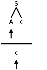
The 2nd condition may seem strange; it did to me for a while.
Let's consider the simplest case that condition 2 is trying to
avoid.
S is the start symbol
    A → ε      // β=ε so β derives ε
    A → c      // α=c so α derives a string beginning with c
    S → A c    // c is in FOLLOW(A)
Probably the simplest derivation possible is
S ⇒ A c ⇒ c
Assume we are using predictive parsing and, as illustrated in the
diagram to the right, we are at A in the parse tree and c in the
input.
Since lookahead=c and c is in FIRST(RHS) for the second A
production, we would choose that production to expand A.
But this is wrong!
Remember that we don't look ahead in the tree, we look ahead just in
the input.
So we would not have noticed that the next node in the tree (i.e.,
in the frontier) is c.
The next node can indeed be c since c is in FOLLOW(A).
So we should have used the top A production to produce ε in
the tree, and then the next node c would match the input c.
Start Lecture #6
Constructing a Predictive Parsing Table
The goal is to produce a table telling us at each situation which
production to apply.
A situation
means a nonterminal in the parse tree and an
input symbol in lookahead.
So we produce a table with rows corresponding to nonterminals and
columns corresponding to input symbols (including $, the endmarker).
In an entry we put the production to apply when we are in that situation.
We start with an empty table M and populate it as follows.
(2e has typo; it has FIRST(A) instead of FIRST(α).)
For each production A → α
- For each terminal a in FIRST(α), add A → α
to M[A,a].
This is what we did with predictive parsing in chapter 2.
The point was that if we are up to A in the tree and a is
the lookahead, we could (should??) use the
production A→α.
- If ε is in FIRST(α), then add
A → α to M[A,b] (resp. M[A,$]) for each
terminal b in FOLLOW(A) (if $ is in FOLLOW(A)).
This is not so obvious; it corresponds to the second
(
strange
) condition above.
If ε is in FIRST(α), then α⇒*ε.
Hence we could (should??) apply the production A→α,
have the α go to ε and then the b (or $) that
follows A will match the b (or $) in the input.
When we have finished filling in the table M, what do we do if an
slot has
- no entries?
This is a normal occurrence and does not indicate a problem with
the table.
Instead, it means that, if parsing gets to this situation, no
production is appropriate.
In other words parsing should never reference this table slot.
Hence, if parsing an input does reference this
entry, that input is not in the language
generated by the grammar.
A production quality parser might try to correct the input, but
for us, it is enough to print an error message and give
up.
- one entry?
Perfect!
This means we know exactly what to do in this situation.
- more than one entry?
This should not happen since the present section is entitled
LL(1) grammars
.
Mostly likely the problem is that the grammar is not LL(1).
(Also possible is that an error was made in constructing the
table.)
Since the grammar is not LL(1), we must use a different
technique instead of predictive parsing.
One possibility is bottom-up parsing, which we study next.
Another possibility is to modify the procedure for this
nonterminal to look further ahead (typically one more token) to
decide what action to perform.
Example: Work out the parsing table for
    E  → T E'
    E' → + T E' | ε
    T  → F T'
    T' → * F T' | ε
    F  → ( E ) | id
| FIRST | FOLLOW |
|---|
| E | ( id | $ ) |
| E' | ε + | $ ) |
| T | ( id | + $ ) |
| T' | ε * | + $ ) |
| F | ( id | * + $ ) |
Nonter-
minal | Input Symbol |
|---|
| + | * | ( | ) | id | $ |
| E | | | | | | |
| E' | | | | | | |
| T | | | | | | |
| T' | | | | | | |
| F | | | | | | |
We already computed FIRST and FOLLOW as shown on the right.
The table skeleton is on the left.
Example: What about ε-productions?
Produce FIRST, FOLLOW, and the parsing table for
    S → B D
    B → b | ε
    D → d | ε
Homework: Produce the predictive parsing table for
- S → 0 S 1 | 0 1
- the prefix grammar S → + S S | * S S | a
Don't forget to eliminate left recursion and perform left factoring
if necessary.
Remark: Lab 3 will use the material up to here.
4.4.4: Nonrecursive Predictive Parsing
This illustrates the standard technique for eliminating recursion
by keeping the stack explicitly.
The runtime improvement can be considerable.
4.4.5: Error Recovery in Predictive Parsing
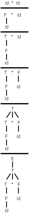
4.5: Bottom-Up Parsing
Now we start with the input string, i.e., the bottom (leaves) of
what will become the parse tree, and work our way up to the start
symbol.
For bottom up parsing, we are not fearful of left recursion as we
were with top down.
Our first few examples will use the left recursive expression
grammar
    E → E + T | T
    T → T * F | F
    F → ( E ) | id
4.5.1: Reductions
Remember that running a production in reverse
, i.e., replacing
the RHS by the LHS, is called reducing.
So our goal is to reduce the input string to the start symbol.
On the right is a movie of parsing id*id in a bottom-up
fashion.
Note the way it is written.
For example, from step 1 to 2, we don't just put F above id*id.
We draw it as we do because it is the current top of the tree (really
forest) and not the bottom that we are working on so we want the top
to be in a horizontal line and hence easy to read.
The tops of the forest are the roots of the subtrees present in the
diagram.
For the movie those are
id * id, F * id, T * id, T * F, T, E
Note that (since the reduction successfully reaches the start
symbol) each of these sets of roots is a sentential form.
The steps from one frame of the movie, when viewed going down the
page, are reductions (replace the RHS of a production by the LHS).
Naturally, when viewed going up the page, we have a derivation
(replace LHS by RHS).
For our example, looking at the top row of each frame, we see that
the derivations are
E ⇒ T ⇒ T * F ⇒ T * id ⇒ F * id ⇒ id * id
Note that this is a rightmost derivation and hence each of
the sets of roots identified above is a right sentential form.
So the reduction we did in the movie was a rightmost derivation in
reverse.
Remember that for a non-ambiguous grammar there is only one
rightmost derivation and hence there is only one rightmost
derivation in reverse.
Remark: You cannot simply scan the string (the
roots of the forest) from left to right and choose the first
substring that matches the RHS of some production.
If you try it in our movie you will reduce T to E right after T
appears.
The result is not a right sentential form.
Right
Sentential
Form | Handle | Reducing
Production |
|---|
| id1 * id2 | id1 | F → id |
| F * id2 | F | T → F |
| T * id2 | id2 | F → id |
| T * F | T * F | T → T * F |
| T | T | E → T |
| E | | |
4.5.2: Handle Pruning
The strings that are reduced during the reverse of a
rightmost derivation are called the handles.
For our example, this is shown in the table on the right.
Note that the string to the right of the handle must contain only
terminals.
If there was a nonterminal to the right, it would have been derived
away in the RIGHTmost derivation that leads to this right sentential
form.
Often instead of referring to a derivation A→α
as a handle, we call α the handle.
I should say a handle because there can be more than one if the
grammar is ambiguous.
However, we are not emphasizing ambiguous grammars.
So (assuming a non-ambiguous grammar) the rightmost derivation in
reverse can be obtained by constantly reducing the handle in the
current string.
Given a grammar how do you find the handle (a handle if the grammar
is ambiguous) of a string (which must be a right sentential form or
there is no handle)?
Answer: Construct the (a if ambiguous, but we are not so interested
in ambiguous grammars) rightmost derivation for the string and the
handle is the last production you applied (so if you are doing
rightmost derivations in reverse, the handle is the first production
you would reduce by).
But how do you find the rightmost derivation?
Good question, we still have work to do.
Homework: 1, 2.
4.5.3: Shift-Reduce Parsing
We use two data structures for these parsers.
- A stack of grammar symbols, terminals and nonterminals.
This stack is drawn in examples as having its top on the right
and bottom on the left.
The items
shifted
(basically pushed, see below) onto the
stack will be terminals, which are subsequently reduced
to nonterminals.
The bottom of the stack is marked with $ and initially the stack
is empty (i.e., has just $).
- An input buffer that (conceptually) holds the remainder of the
input, i.e., the part that has yet to be shifted onto the stack.
An endmarker $ is placed after the end of the input.
Initially the input buffer contains the entire input followed by
$.
(In practice we use some more sophisticated buffering technique,
as we saw in section 3.2 with buffers pairs that does not require
having the entire input in memory at once.)
| Stack | Input | Action |
|---|
| $ | id1*id2$ | shift |
| $id1 | *id2$ | reduce F→id |
| $F | *id2$ | reduce T→F |
| $T | *id2$ | shift |
| $T* | id2$ | shift |
| $T*id2 | $ | reduce F→id |
| $T*F | $ | reduce T→T*F |
| $T | $ | reduce E→T |
| $E | $ | accept |
The idea, illustrated by the table on the right, is that at any
point the parser can perform one of four operations.
- The parser can shift a symbol from the beginning of the input
onto the TOS.
- If the TOS is a handle, the parser can reduce it to its LHS.
- If the parser reaches the state where the stack is $S (S is
the start symbol) and the input is $, the parser terminates
successfully.
- The parser reaches an error state, where neither shifting nor
reducing are possible.
A technical point, which explains the usage of a stack is that a
handle is always at the TOS.
See the book for a proof; the idea is to look at what rightmost
derivations can do (specifically two consecutive productions) and
then trace back what the parser will do since it does the reverse
operations (reductions) in the reverse order.
We have not yet discussed how to decide whether to shift or reduce
when both are possible.
We have also not discussed which reduction to choose if multiple
reductions are possible.
These are crucial question for bottom up (shift-reduce) parsing and
will be addressed.
Homework: 3.
4.5.4: Conflicts During Shift-Reduce Parsing
There are grammars (non-LR) for which no viable algorithm can
decide whether to shift or reduce when both are possible or which
reduction to perform when several are possible.
However, for most languages, choosing a good lexer yields an LR(k)
language of tokens.
For example, ada uses () for both function calls and array
references.
If the lexer returned id for both array names and procedure names
then a reduce/reduce conflict would occur when the stack was
... id ( id
and the input was
) ...
since the id on TOS should be reduced to parameter if the first id
was a procedure name and to expr if the first id was an array name.
A better lexer (and an assumption, which is true in ada, that the
declaration must precede the use) would return proc-id when it
encounters a lexeme corresponding to a procedure name.
It does this by consulting tables that it builds.
4.6: Introduction to LR Parsing: Simple LR
I will have much more to say about SLR (simple LR) than the other
LR schemes.
The reason is that SLR is simpler to understand, but does capture
the essence of shift-reduce, bottom-up parsing.
The disadvantage of SLR is that there are LR grammars that are not
SLR.
4.6.1: Why LR Parsers?
The text's presentation is somewhat controversial.
Most commercial compilers use hand-written top-down parsers of the
recursive-descent (LL not LR) variety.
Since the grammars for these languages are not LL(1), the
straightforward application of the techniques we have seen will not
work.
Instead the parsers actually look ahead further than one token, but
only at those few places where the grammar is in fact not LL(1).
Recall that (hand written) recursive descent compilers have a
procedure for each nonterminal so we can customize as needed
.
These compiler writers claim that they are able to produce much
better error messages than can readily be obtained by going to LR
(with its attendant requirement that a parser-generator be used since
the parsers are too large to construct by hand).
Note that compiler error messages are a very important user interface
issue and that with recursive descent one can augment the procedure
for a nonterminal with statements like
if (nextToken == X) then error(expected Y here
)
Nonetheless, the claims made by the text are correct, namely.
- LR parsers can be constructed to recognize nearly all
programming-language constructs for which CFGs exist.
- LR-parsing is the most general non-backtracking, shift-reduce
method known, yet can be implemented relatively efficiently.
- LR-parsing can detect a syntactic error as soon as possible.
- LR grammars can describe more languages than LL grammars.
4.6.2: Items and the LR(0) Automaton
We now come to grips with the big question
:
How does a shift-reduce parser know when to shift and when to
reduce?
This will take a while to answer in a satisfactory manner.
The unsatisfactory answer is that the parser has tables that say in
each situation
whether to shift or reduce (or announce error,
or announce acceptance).
To begin the path toward the answer, we need several definitions.
An item is a production with a marker saying how far the parser has
gotten with this production.
Formally,
Definition: An (LR(0)) item
of a grammar is a production with a dot added somewhere to the RHS.
Note: A production with n symbols on the RHS,
generates n+1 items.
Examples:
- E → E + T generates 4 items.
- E → · E + T
- E → E · + T
- E → E + · T
- E → E + T ·
- A → ε generates A → · as its only item.
The item E → E · + T signifies that the parser has just
processed input that is derivable from E (i.e., reducible to E) and
will look for input derivable from + T.
The item E → E + T · indicates that the parser has seen
the entire RHS and must consider reducing it to E.
Important: consider reducing
does not mean
reduce
.
The parser groups certain items together into states.
As we shall see, the items within a given state are treated similarly.
Our goal is to construct first the canonical LR(0)
collection of states and then a DFA called the LR(0) automaton
(technically not a DFA since it has no dead state
).
To construct the canonical LR(0) collection formally and present
the parsing algorithm in detail we shall
- augment the grammar
- define functions CLOSURE and GOTO
Augmenting the grammar is easy.
We simply add a new start state S' and one production
S'→S.
The purpose is to detect success, which occurs when the parser is
ready to reduce S to S'.
So our example grammar
    E → E + T | T
    T → T * F | F
    F → ( E ) | id
is augmented by adding the production E' → E.
Interlude: The NFA Behind the Scenes
I hope the following interlude will prove helpful.
When I was first preparing to present SLR a few years ago, I was
struck by how much it looked like we were working with a DFA that
came from some (unspecified and unmentioned) NFA.
It seemed that by first doing the NFA, I could give some insight,
especially since that is how we proceeded last chapter with lexers.
Since our current example would generate an NFA with many states
and hence a big diagram, let's consider instead the following
extremely simple grammar.
    E → E + T
    E → T
    T → id
When augmented this becomes
    E' → E
    E  → E + T
    E  → T
    T  → id
When the dots are added we get 10 items (4 from the second
production, 2 each from the other three).
See the diagram at the right.
We begin at E' → · E since it is the
start item.
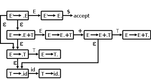 Note that there are four
 kinds
of edges.
- Edges labeled with terminals.
These correspond to shift actions, where the indicated terminal
is shifted from the input to the stack.
- Edges labeled with nonterminals.
These will correspond to reduce actions when we construct the
DFA.
The stack is reduced
by a production having the given nonterminal as LHS.
Reduce actions do more as we shall see.
- Edges labeled with ε.
These are associated with the closure operation to be discussed
and are the source of the nondeterminism (i.e., why the diagram
is an NFA).
- An edge labeled $.
used when we are reducing via the E'→E production and
This edge, which can be thought of as shifting the endmarker, is
accepting the input.
If we are at the item E→E·+T (the dot indicating that
we have seen an E and now need a +) and then shift a + from the
input to the stack, we move to the item E→E+·T.
If the dot is before a nonterminal, the parser needs a reduction
with that nonterminal as the LHS.
Now we come to the idea of closure, which I illustrate in the
diagram with the ε's.
I hope this will help you understand the idea of closure,
which like ε in regular expressions, leads to nondeterminism.
Look at the start state.
The placement of the dot indicates that we next need to see an E.
Since E is a nonterminal, we won't see it in the input, but will
instead have to generate it via a production.
Thus by looking for an E, we are also looking for any production
that has E on the LHS.
This is indicated by the two ε's leaving the top left box.
Similarly, there are ε's leaving the other three boxes where
the dot is immediately to the left of a nonterminal.
Remark: Perhaps instead of saying also looking
for
I should say really looking for
.

As with regular expressions, we combine n-items
connected by
an ε arc into a d-item
.
The actual terminology used is that we combine these items into a
set of items (later referred to as a state).
For example all four items in the left column of the diagram above
are combined into the state or item set labelled I0 in
the diagram on the right.
There is another combination that occurs.
The top two n-items in the left column of the diagram above both
have E transitions (outgoing arcs labeled E).
Since we are considering these two n-items to be the same d-item and
the arcs correspond to the same transition, the two targets (the top
two n-items in the 2nd column of the diagram above) are combined.
A d-item has all the outgoing arcs of the original n-items it
contains.
This is the way we converted an NFA into a DFA via the subset
algorithm described in the previous chapter.
I0, I1, etc are called (LR(0)) item sets.
The DFA containing these item sets as states and the state
transitions described above is called the LR(0) automaton.
| Stack | Symbols | Input | Action |
|---|
| $0 | | id+id$ | Shift to 3 |
| $03 | id | +id$ | Reduce by T→id |
| $02 | T | +id$ | Reduce by E→T. |
| $01 | E | +id$ | Shift to 4 |
| $014 | E+ | id$ | Shift to 3 |
| $0143 | E+id | $ | Reduce by T→id |
| $0145 | E+T | $ | Reduce by E→E+T |
| $01 | E | $ | Accept |
Now we put the automaton to use to parse id+id as shown in the table
on the right.
The Input and Action columns are as in
the previous table.
In that table input symbols were shifted onto the stack where they
were reduced, eventually producing the start symbol.
In the present table the symbols column has this property, but is
actually not used in shift reducing parsing.
I include it for clarity.
Instead the stack column (in the new table) records the states we
have shifted into.
A reduction (which removes symbols previously shifted and inserts
the LHS symbol) has the corresponding effect on the stack: the
states corresponding the the RHS items are popped and the state
corresponding the LHS item is pushed.
We start in the initial state with the symbols column empty and the
input full.
The $'s are just end markers.
From state 0, called I0 in my diagram (following the book they are
called I's since they are sets of items), we can only shift in the
id (the nonterminals will appear in the symbols column).
This brings us to I3 so we push a 3 onto the stack
In I3 we first notice that there is no outgoing arc labeled with a
terminal; hence we cannot do a shift.
However, we do see a completed production in the box (the dot is on
the extreme right).
Since the RHS consists solely of terminals, having the dot at the
end means that we have seen (i.e., shifted) in the input the entire
RHS of this production and are ready to perform a reduction.
To reduce we pop the stack for each symbol in the RHS since we are
replacing the RHS by the LHS.
This time the RHS has one symbol so we pop the stack once and also
remove one symbol from the symbols column.
The stack corresponds to moves (i.e., state transtions) so we are
undoing the move to 3 and we are temporarily
in 0 again.
But the production has a T on the LHS so we follow the T transition
from 0 to 2, push T onto Symbols, and push 2 on.to the stack.
In I2 we again see no possible shift, but again do see a completed
production.
This time the RHS contains a nonterminal so is not simply the
result of shifting in symbols, but also reflects previous
reductions.
We again perform the indicated reduction, which takes us to I1
You might think that at I1 we could reduce using the completed
bottom production, but that is wrong.
This item (E'→E·) is special and can only be
applied when we are at the end of the input string.
Thus the next two steps are shifts of + and id, sending us to 3
again, where, as before, we have no choice but to reduce the id to T
and are in step 5 ready for the
big one
.
The production in 5 has three symbols on the RHS so we pop (back up)
three times again temporarily landing in 0, but the RHS puts us in 1.
Perfect!
We have just E as a symbol and the input is empty so we are ready to
reduce by E'→E, which signifies acceptance.
Now we rejoin the book and say it more formally.
Actually there is more than mere formality coming.
For the example above, we had no choices, but that was because the
example was simple.
We need more machinery to insure that we never have two or more
possible moves to choose among.
Specifically, we will need FOLLOW sets, the same ones we calculated
for top-down parsing.
Closure of Item Sets
Say I is a set of items and one of these items is
A→α·Bβ.
This item represents the parser having seen α and records that
the parser might soon see the remainder of the RHS.
For that to happen the parser must first see a string derivable from
B.
Now consider any production starting with B, say B→γ.
If the parser is to make progress on
A→α·Bβ, it will need to be making
progress on one such B→·γ.
Hence we want to add all the latter productions to any state that
contains the former.
We formalize this into the notion of closure.
For any set of items I, CLOSURE(I) is formed as follows.
- Initialize CLOSURE(I) = I
- If A → α · B β is in
CLOSURE(I) and B → γ is a production, then
add B → · γ to the closure and repeat.
Example:
Recall our main example
    E' → E
    E  → E + T | T
    T  → T * F | F
    F  → ( E ) | id
CLOSURE({E' → · E})
contains 7 elements.
The 6 new elements are the 6 original productions each with a dot
right after the arrow.
Make sure you understand why all 6 original
productions are added.
It is not because the E'→E production is special.
The Function GOTO
If X is a grammar symbol, then moving from
A→α·Xβ to A→αX·β
signifies that the parser has just processed (input derivable from)
X.
The parser was in the former position and (input derivable from) X
was on the input; this caused the parser to go to the latter
position.
We (almost) indicate this by writing
GOTO(A→α·Xβ,X) is
A→αX·β.
I said almost because GOTO is actually defined from item sets to
item sets not from items to items.
Definition: If I is an item set and X is a
grammar symbol, then GOTO(I,X) is the closure of the set of items
A→αX·β where A→α·Xβ is
in I.
The Canonical Collection of LR(0) Items—the LR(0) Automaton
I really believe this is very clear, but I understand that the
formalism makes it seem confusing.
Let me begin with the idea.
We augment the grammar and get this one new production; take its
closure.
That is the first element of the collection; call it I0.
Try GOTOing from I0, i.e., for each grammar symbol,
consider GOTO(I0,X); each of these (almost) is another
element of the collection.
Now try GOTOing from each of these new elements of the collection,
etc.
Start with jane smith, add all her friends F, then add the friends
of everyone in F, called FF, then add all the friends of everyone in
FF, etc
The (almost)
is because GOTO(I0,X) could be
empty so formally we construct the canonical collection of LR(0)
items, C, as follows
- Initialize C = CLOSURE({S' → S})
- If I is in C, X is a grammar symbol, and GOTO(I,X)≠φ
then add it to C and repeat.
This GOTO gives exactly the arcs in the DFA I constructed earlier.
The formal treatment does not include the NFA, but works with the
DFA from the beginning.
Definition: The above collection of
item sets (so this is a set of sets) is called the canonical
LR(0) collection and the DFA having this collection as
nodes and the GOTO function as arcs is called the
LR(0) automaton.
Homework:
Construct the LR(0) automaton for the following grammar (which
produces simple postfix expressions).
S → S S + | S S * | a
Don't forget to augment the grammar.
Since this is bottom-up parsing, the left recursion is
not a problem.
Start Lecture #7
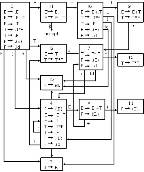
The DFA for our Main Example
Our main example
    E' → E
    E  → E + T | T
    T  → T * F | F
    F  → ( E ) | id
is larger than the toy I did before.
The NFA would have 2+4+2+4+2+4+2=20 states (a production with k
symbols on the RHS gives k+1 N-states since there k+1 places to
place the dot).
This gives rise to 12 D-states.
However, the development in the book, which we are following now,
constructs the DFA directly.
The resulting diagram is on the right.
Start constructing the diagram on the board:
Begin with {E' → ·E},
take the closure, and then keep applying GOTO.
Use of the LR(0) Automaton
A state of the automaton is an item set as described previously.
The transition function is GOTO.
If during a parse we are up to item set Ij (often called
state sj or simply state j) and the next input symbol is
b (it of course must be a terminal), and state j has an outgoing
transition labeled b, then the parser shifts b to the stack
.
Actually, although b is removed from the input string, what is
pushed on the stack is k, the destination state of the transition
labeled b.
If there is no such transition, then the parser performs a
reduction; choosing which reduction to use is determined by the
items in Ij and the FOLLOW sets.
(It is also possible that the parser will now accept the input
string or announce that the input string is not in the
language).
SLR Parsing Using the Diagram and FOLLOW
Naturally, programs can't use diagrams so we will construct a
table, but it is instructive to see how the LR(0) diagram plus the
FOLLOW sets we have see before are enough for SLR parsing.
The diagram and FOLLOW sets (plus the production list and the
ACTION/GOTO table) can be
see here.
For now just use the diagram and FOLLOW.
Take a legal input, e.g. id+id*id, and shift whenever the
diagram says you can and, when you can't, reduce using the
unique completed item having the input symbol in
FOLLOW.
Don't forget that reducing means backing up the number of grammar
symbols in the RHS and then going forward using the arc labeled with
the LHS.
4.6.3: The LR-Parsing Algorithm
The LR-parsing algorithm must decide when to shift and when to
reduce (and in the latter case, by which production).
It does this by consulting two tables, ACTION and GOTO.
The basic algorithm is the same for all LR parsers, what changes are
the tables ACTION and GOTO.
The LR Parsing Tables
We have already seen GOTO (for SLR).
Remark: Technical point that may, and probably
should, be ignored: our GOTO was defined on pairs
[item-set,grammar-symbol].
The new GOTO is defined on pairs [state,nonterminal].
A state is simply an item set (so nothing is new here).
We will not use the new GOTO on terminals so we just define it on
nonterminals.
Given a state i and a terminal a (or the endmarker), ACTION[i,a]
can be
- Shift j.
The terminal a is shifted on to the stack and the parser enters
state j.
- Reduce A → α.
The parser reduces α on the TOS to A.
- Accept.
- Error
So ACTION is the key to deciding shift vs. reduce.
We will soon see how this table is computed for SLR.
Since ACTION is defined on [state,terminal] pairs and GOTO is
defined on [state,nonterminal] pairs, we can combine these tables
into one defined on [state,grammar-symbol] pairs.
LR-Parser Configurations (formalism)
This formalism is useful for stating the actions of the parser
precisely, but I believe the parser can be explained without this
formalism.
The essential idea of the formalism is that the entire state of the
parser can be represented by the vector of states on the stack
and input symbols not yet processed.
As mentioned above the Symbols column is redundant so a
configuration of the parser consists of the current stack and the
remainder of the input.
Formally it is
(s0,s1...sm,aiai+1...an$)
where the s's are states and the a's input symbols.
This configuration could also be represented by the
right-sentential form
X1...Xm,ai...an
where the X is the symbol associated with the state.
X is either the terminal just shifted in or the LHS of the
reduction just performed.
Behavior of the LR Parser
The parser consults the combined ACTION-GOTO table for its current
state (TOS) and next input symbol, formally this is
ACTION[sm,ai], and proceeds based on the value
in the table.
If the action is a shift, the next state is clear from the DFA
We have done this informally just above; here we use the formal
treatment).
- Shift s.
The input symbol a is pushed and s becomes the new state.
The new configuration is
(s0...sms,ai+1...an)
- Reduce A → α.
Let r be the number of symbols in the RHS of the production.
The parser pops r items off the stack (backing up r states) and
enters the state GOTO(sm-r,A).
That is after backing up it goes where A says to go.
A real parser would now probably do something, e.g., build a
tree node or perform a semantic action.
Although we know about this from the chapter 2 overview, we
don't officially know about it here.
So for now think of it simply printing the production the parser
reduced by.
- Accept.
- Error.
4.6.4 Constructing SLR-Parsing Tables
The missing piece of the puzzle is finally revealed.
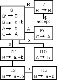
A Simple (but fake) Example
| State | a | b | + | $ | A | B | C |
|---|
| 7 | | | | acc | | | |
| 8 | s11 | s10 | | | 9 | 7 | |
| 9 | | | | | | | |
| 10 | | | | | | | |
| 11 | | | s12 | | | | |
| 12 | | s13 | | | | | |
| 13 | | r2 | | | | | |
Before defining the ACTION and GOTO tables precisely, I want to do
it informally via the simple example on the right.
This is a FAKE example, the B'→·B item
would be in I0 and would have only B→·a+b
with it.
IMPORTANT: To construct the table, you do need
something not in the diagram, namely the FOLLOW sets from top-down
parsing.
For convenience number the productions of the grammar to make them
easy to reference and assume that the production B → a+b is
numbered 2.
Also assume FOLLOW(B)={b} and all other follow sets are empty.
Again, I am not claiming that there is a grammar with this diagram
and these FOLLOW sets.
Show how to calculate every entry in the table using the diagram
and the FOLLOW sets.
Then consider input a+b
and see how the table guides to
eventually accepting the a+b
string.
The Action-GOTO Table
This table is the SLR equivalent of the predictive-parsing table we
constructed for top-down parsing.
The action table is defined with states (item sets) as rows and
terminals and the $ endmarker as columns.
GOTO has the same rows, but has nonterminals as
columns.
So we construct a combined ACTION-GOTO table, with states as rows
and grammar symbols (terminals + nonterminals) plus $ as columns.
- Each arc in the diagram labeled with a terminal indicates a
shift.
In the entry with row the state at the tail of the arc and
column the labeling terminal place sn, where n is the
state at the head of the arc.
This indicates that if we are in the given state and the input
is the given terminal, we shift to new state n.
- Each arc in the diagram labeled with a nonterminal informs us
what state to enter if we reduce.
In the entry with row the state at the tail of the arc and
column the labeling nonterminal place n, where n is the state
at the head of the arc.
- Each completed item (dot at the extreme right) indicates
a possible reduction.
In each entry with row the state containing the completed
item and column a terminal in the FOLLOW set of the LHS of
the production corresponding to this item, place rn, where n is
the number of the production.
(In particular, at entry [13,b] place an r2.).
- In the entry with row (i.e., state) containing S'→S and
column $, place
accept
.
- If any entry is labelled twice (i.e., a conflict) the grammar
is not SLR(1).
- Any unlabeled entry corresponds to an input error.
If the parser accesses this entry, the input sentence is not in
the language generated by the grammar.
A Terminology Point
The book (both editions) and the rest of the world seem to use GOTO
for both the function defined on item sets and the derived function
on states.
As a result we will be defining GOTO in terms of GOTO.
Item sets are denoted by I or Ij, etc.
States are denoted by s or si or i.
Indeed both books use i in this section.
The advantage is that on the stack we placed integers (i.e., i's) so
this is consistent.
The disadvantage is that we are defining GOTO(i,A) in terms of
GOTO(Ii,A), which looks confusing.
Actually, we view the old GOTO as a function and the new one as an
array (mathematically, they are the same) so we actually write
GOTO(i,A) and GOTO[Ii,A].
The Table Construction Algorithm
The diagrams above are constructed for our use; they are not used in
constructing a bottom-up parser.
Here is the real algorithm, which uses just the augmented grammar
(i.e., after adding S' → S) and the FOLLOW sets.
- Construct the LR(0) automaton with states
{I0,...,In} and transition function GOTO.
- The parsing actions for state i.
- If A→α·bβ is in Ii for
b a terminal, then ACTION[i,b]=
shift j
, where
GOTO(Ii,b)=Ij.
- If A→α· is in Ii, for
A≠S', then, for all b in FOLLOW(A),
ACTION[i,b]=
reduce A→α
.
- If S'→S· is in Ii, then
ACTION[I,$]=
accept
.
- If any conflicts occurred, the grammar is not SLR(1).
- If GOTO(Ii,A)=Ij, for a nonterminal A,
then GOTO[i,A]=j.
- All entries not yet defined are
error
.
- The initial state is the one containing S'→·S.
The Main Example
Action-GOTO Table
| State | ACTION | GOTO |
|---|
| id | + | * | ( | ) | $ | E | T | F |
|---|
| 0 | s5 | | | s4 | | | 1 | 2 | 3 |
| 1 | | s6 | | | | acc | | | |
| 2 | | r2 | s7 | | r2 | r2 | | | |
| 3 | | r4 | r4 | | r4 | r4 | | | |
| 4 | s5 | | | s4 | | | 8 | 2 | 3 |
| 5 | | r6 | r6 | | r6 | r6 | | | |
| 6 | s5 | | | s4 | | | | 9 | 3 |
| 7 | s5 | | | s4 | | | | | 10 |
| 8 | | s6 | | | s11 | | | | |
| 9 | | r1 | s7 | | r1 | r1 | | | |
| 10 | | r3 | r3 | | r3 | r3 | | | |
| 11 | | r5 | r5 | | r5 | r5 | | | |
- E' → E
- E → E + T
- E → T
- T → T * F
- T → F
- F → ( E )
- F → id
Productions
| FIRST | FOLLOW |
|---|
| E' | ( id | $ |
| E | ( id | + ) $ |
| T | ( id | * + ) $ |
| F | ( id | * + ) $ |
Our main example, pictured on the right, gives the table shown on
the left.
The productions and FOLLOW sets are shown as well (the FIRST sets
are not used directly, but are needed to calculate FOLLOW).
The table entry s5 abbreviates shift and go to state 5
.
The table entry r2 abbreviates reduce by production number 2
,
where we have numbered the productions as shown.
The shift actions can be read directly off the DFA.
For example I1 with a + goes to I6, I6 with an id goes to I5, and I9
with a * goes to I7.
The reduce actions require FOLLOW, which for this simple grammar is
fairly easy to calculate.
Consider I5={F→id·}.
Since the dot is at the end, we are ready to reduce, but we must
check if the next symbol can follow the F we are reducing to.
Since FOLLOW(F)={+,*,),$}, in row 5 (for I5) we put
r6 (for reduce by production 6
) in the columns for
+, *, ), and $.
The GOTO columns can also be read directly off the DFA.
Since there is an E-transition (arc labeled E) from I0
to I1, the column labeled E in row 0 contains a 1.
Since the column labeled + is blank for row 7, we see that it would
be an error if we arrived in state 7 when the next input character
is +.
Finally, if we are in state 1 when the input is exhausted ($ is the
next input character), then we have a successfully parsed the
input.
| Stack | Symbols | Input | Action |
|---|
| 0 | | id*id+id$ | shift |
| 05 | id | *id+id$ | reduce by F→id |
| 03 | F | *id+id$ | reduct by T→id |
| 02 | T | *id+id$ | shift |
| 027 | T* | id+id$ | shift |
| 0275 | T*id | +id$ | reduce by F→id |
| 027 10 | T*F | +id$ | reduce by T→T*F |
| 02 | T | +id$ | reduce by E→T |
| 01 | E | +id$ | shift |
| 016 | E+ | id$ | shift |
| 0165 | E+id | $ | reduce by F→id |
| 0163 | E+F | $ | reduce by T→F |
| 0169 | E+T | $ | reduce by E→E+T |
| 01 | E | $ | accept |
Example:
The diagram on the right shows the actions when SLR is parsing
id*id+id.
On the blackboard let's do id+id*id and see how the precedence is
handled.
Homework: 2 (you already constructed the LR(0)
automaton for this example in the previous homework), 3,
4 (this problem refers to 4.2.2(a-g); only use 4.2.2(a-c).
Example:
What about ε-productions?
Let's do
    A → B D
    B → b B | ε
    D → d
Reducing by the ε-production actually adds a state to the
stack (it pops ZERO states since there are zero symbols on RHS and
pushes one).
Homework: Do the following extension
    A → B D
    B → b B | ε
    D → d D | ε
4.6.5: Viable Prefixes
4.7: More Powerful LR Parsers
We consider very briefly two alternatives to SLR,
canonical-LR or LR, and lookahead-LR or LALR.
4.7.1: Canonical LR(1) Items
SLR used the LR(0) items, that is the items used were productions
with an embedded dot, but contained no other (lookahead)
information.
The LR(1) items contain the same productions with embedded dots, but
add a second component, which is a terminal (or $).
This second component becomes important only when the dot is at the
extreme right (indicating that a reduction can be made if the input
symbol is in the appropriate FOLLOW set).
For LR(1) we do that reduction only if the input symbol is exactly
the second component of the item.
This finer control of when to perform reductions, enables the
parsing of a larger class of languages.
4.7.2: Constructing LR(1) Sets of Items
4.7.3: Canonical LR(1) Parsing Tables
4.7.4: Constructing LALR Parsing Tables
For LALR we merge various LR(1) item sets together, obtaining
nearly the LR(0) item sets we used in SLR.
LR(1) items have two components, the first, called the core, is a
production with a dot; the second a terminal.
For LALR we merge all the item sets that have the same set of cores
by combining the 2nd components of items with like cores (thus
permitting reductions when any of these terminals is the next input
symbol).
Thus we obtain the same number of states (item sets) as in SLR since
only the cores distinguish item sets.
Unlike SLR, we limit reductions to occurring only for certain
specified input symbols.
LR(1) gives finer control; it is possible for the LALR merger to
have reduce-reduce conflicts when the LR(1) items on which it is
based is conflict free.
Although these conflicts are possible, they are rare and the size
reduction from LR(1) to LALR is quite large.
LALR is the current method of choice for bottom-up, shift-reduce
parsing.
4.7.5: Efficient Construction of LALR Parsing Tables
4.7.6: Compaction of LR Parsing Tables
4.8: Using Ambiguous Grammars
4.8.1: Precedence and Associativity to Resolve Conflicts
4.8.2: The Dangling-Else
Ambiguity
4.8.3: Error Recovery in LR Parsing
4.9: Parser Generators
4.9.1: The Parser Generator Yacc
The tool corresponding to Lex for parsing is yacc, which (at least
originally) stood for yet another compiler compiler.
This name is cute but somewhat misleading since yacc (like the
previous compiler compilers) does not produce a complete compiler,
just a parser.
The structure of the yacc user input is similar to that for lex,
but instead of regular definitions, one includes productions with
semantic actions.
There are ways to specify associativity and precedence of
operators.
It is not done with multiple grammar symbols as in a pure parser,
but more like declarations.
Use of Yacc requires a serious session with its manual.
4.9.2: Using Yacc with Ambiguous Grammars
Creating Yacc Lexical Analyzers with Lex
4.9.4: Error Recovery in Yacc
Chapter 5: Syntax-Directed Translation
Homework: Read Chapter 5.
Again we are redoing, more formally and completely, things we
briefly discussed when breezing over chapter 2.
Recall that a syntax-directed definition (SDD) adds semantic rules
to the productions of a grammar.
For example to the production T → T / F we might
add the rule
T.code = T1.code || F.code || '/'
if we were doing an infix to postfix translator.
Rather than constantly copying ever larger strings to finally
output at the root of the tree after a depth first traversal, we can
perform the output incrementally by embedding semantic actions
within the productions themselves.
The above example becomes
T → T1 / F { print '/' }
Since we are generating postfix, the action comes at the end (after
we have generated the subtrees for T1 and F, and hence
performed their actions).
In general the actions occur within the production, not necessarily
after the last symbol.
For SDD's we conceptually need to have the entire tree available
after the parse so that we can run the postorder traversal.
(It was postorder for the infix→postfix translator since we had
a simple S-attributed
SDD.
We will traverse the parse tree in
other orders when the SDD is not S-attributed, and will see
situations when no traversal order is possible.)
In some situations semantic actions can be performed during the
parse, without saving the tree.
However, this does not occur for large commercial compilers since
they make several passes over the tree for optimizations.
We will not make use of this possibility either; your lab 3 (parser)
will produce a tree and your lab 4 (semantic analyzer / intermediate
code generator) will read this tree and perform the semantic rules
specified by the SDD.
5.1: Syntax-Directed Definitions (SDDs)
Formally, attributes are values (of any type) that are associated
with grammar symbols.
Write X.a for the attribute a of symbol X.
You can think of attributes as fields in a record/struct/object.
Semantic rules (rules for short) are associated with productions
and give formulas to calculate attributes of nonterminals in the
production.
5.1.1: Inherited and Synthesized Attributes
Terminals can have synthesized attributes (not yet officially
defined); these are given to it by the lexer (not the parser).
For example the token id might well have the
attribute lexeme, where id.lexeme is the lexeme
that the lexer converted into this instance of id.
There are no rules in an SDD giving attribute values to terminals.
Terminals do not have inherited attributes (to be defined shortly).
A nonterminal B can have both inherited and synthesized attributes.
The difference is how they are computed.
In either case the computation is specified by a rule associated
with the production at a node N of the parse tree.
Definition:
A synthesized attribute of a nonterminal B is
defined at a node N where B is the LHS of the production associated
with N.
The attribute can depend on only (synthesized or inherited)
attribute values at the children of N (the RHS of the production)
and on inherited attribute values at N itself.
The arithmetic division example above was synthesized.
| Production | Semantic Rules |
|---|
| L → E $ | L.val = E.val |
| E → E1 + T | E.val = E1.val + T.val |
| E → E1 - T | E.val = E1.val - T.val |
| E → T | E.val = T.val |
| T → T1 * F | T.val = T1.val * F.val |
| T → T1 / F | T.val = T1.val / F.val |
| T → F | T.val = F.val |
| F → ( E ) | F.val = E.val |
| F → num | F.val = num.lexval |
Example:
The SDD at the right gives a left-recursive grammar for
expressions with an extra nonterminal L added as the start symbol.
The terminal num is given a value by the lexer,
which corresponds to the value stored in the numbers table for lab 2.
Draw the parse tree for 7+6/3 on the board and verify that L.val is
9, the value of the expression.
This example uses only synthesized attributes.
Definition: An SDD with only
synthesized attributes is called S-attributed.
For these SDDs all attributes depend only on attribute values at
the children.
Why?
Answer: The other possibility (depending on values at the node
itself) involves inherited attributes, which are absent in an
S-attributed SDD.
Thus, for an S-attributed SDD, all the rules can be evaluated by a
single bottom-up (i.e., postorder) traversal of the annotated parse
tree.
Inherited attributes are more complicated since the node N of the
parse tree with which the attribute is associated (and which is also
the natural node to store the value) does not contain the production
with the corresponding semantic rule.
Definition:
An inherited attribute of a nonterminal B at node
N, where B is the LHS of the production, is defined by a semantic
rule of the production at the parent of N (where B
occurs in the RHS of the production).
The value depends only on attributes at N, N's siblings, and N's
parent.
Note that when viewed from the parent node P (the site of the
semantic rule), the inherited attribute depends on values at P and
at P's children (the same as for synthesized attributes).
However, and this is crucial, the nonterminal B is the LHS of a child
of P and hence the attribute is naturally associated with that child.
It is normally stored there and is shown there in the diagrams below.
We will soon see examples with inherited attributes.
Definition: Often the attributes are
just evaluations without side effects.
In such cases we call the SDD an
attribute grammar.
Start Lecture #8
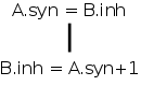
5.1.2: Evaluating an SDD at the Nodes of a Parse Tree
If we are given an SDD and a parse tree for a given sentence, we
would like to evaluate the annotations at every node.
Since, for synthesized annotations parents can depend on children,
and for inherited annotations children can depend on parents, there
is no guarantee that one can in fact find an order of evaluation.
The simplest counterexample is the single production A→B with
synthesized attribute A.syn, inherited attribute B.inh, and rules
A.syn=B.inh and B.inh=A.syn+1.
This means to evaluate A.syn at the parent node we need B.inh at the child
and vice versa.
Even worse it is very hard to tell, in general, if every sentence
has a successful evaluation order.
All this not withstanding we will not have great difficulty because
we will not be considering the general case.
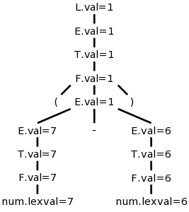
Annotated Parse Trees
Recall that a parse tree has leaves that are terminals and internal
nodes that are nonterminals.
Definition: A parse tree decorated
with attributes, is called an annotated parse tree.
It is constructed as follows.
Each internal node corresponds to a production.
The node is labeled with the LHS of the production.
If there are no attributes for the LHS in this production, we leave
the node as it was (I don't believe this is a common occurrence).
If there are k attributes for the LHS, we replace the LHS in the
parse tree by k equations.
The LHS of the equation is the attribute and the right hand side is
its value.
Note that the annotated parse tree contains all the information of
the original parse tree since we (either leave the node
alone—if the LHS had no attributes or) replace the
nonterminal A labeling the LHS with a series of equations
A.attr=value.
We computed the values to put in this tree for 7+6/3 and on the
right is (7-6).
Homework: 1
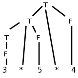
Why Have Inherited Attributes?
Inherited attributed definitely make the situation more
complicated.
For a simple example, recall the circular dependency above involving
A.syn and B.inh.
But we do need them.
Consider the following left-recursive grammar for multiplication of
numbers, and the parse tree on the right for 3*5*4.
    T → T * F
    T → F
    F → num
It is easy to see how the values can be propagated up the tree and
the expression evaluated.
When doing top-down parsing, however, we need to avoid left
recursion.
Consider the grammar below, which is the result of removing the left
recursion.
Again its parse tree is shown on the right.
Try not to look at the semantic rules for the moment.
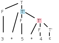
| Production | Semantic Rules | Type |
|---|
| T → F T' | T'.lval = F.val | Inherited |
| T.val = T'.tval | Synthesized |
| T' → * F T1'
| T'1.lval = T'.lval * F.val | Inherited
|
| T'.tval = T'1.tval | Synthesized |
| T' → ε | T'.tval = T'.lval | Synthesized |
| F → num | F.val = num.lexval | Synthesized |
Where on the tree should we do the multiplication 3*5 since
there is no node that has 3 and * and 5 as children?
The second production is the one with the *, so that is the natural
candidate for the multiplication site.
Make sure you see that this production (for the * in 3*5) is
associated with the blue-highlighted node in the parse tree.
The right operand (5) can be obtained from the F that is the middle
child of this T'.
F gets the value from its child, the number itself; this is an
example of the simple synthesized case we have already seen,
F.val=num.lexval (see the last semantic rule in the table).
But where is the left operand?
It is located at the sibling of T' in the parse
tree, i.e., at the F immediately to T's left (we shall see the
significance that the sibling is to the left; it is not significant
that it is immediately to the left).
This F is not mentioned in the production associated with the
T' node we are examining.
So, how does T' get F.val from its sibling?
Answer: The common parent, in this case T, can get the value from F
and then our node can inherit the value from its parent.
Bingo! ... an inherited attribute.
This can be accomplished by having the following rule at the node
T.
T'.lval = F.val (inherited)
This observation yields the first rule in the table.
Now lets look at the second multiplication (3*5)*4, where the
parent of T' is another T'.
(This is the normal case. When there are n multiplies,
n-1 have T' as parent and only one has T).
The pink-highlighted T' is the site for the multiplication.
However, it needs as left operand, the product 3*5
that its parent can calculate.
So we have the parent (another T' node, the blue one in this
case) calculate the product and store it as an attribute of
its right child namely the pink T'.
That is the first rule for T' in the table.
We have now explained the first, third, and last semantic rules.
These are enough to calculate the answer.
Indeed, if we trace it through, 60 does get evaluated and stored in
the bottom right T', the one associated with the ε-production.
Our remaining goal is to get the value up to the root where it
represents the evaluation of this term T and can be combined with
other terms to get the value of a larger expression.
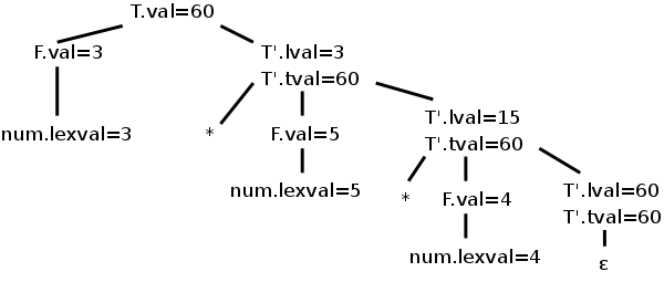
Going up is easy, just synthesize.
I named the attribute tval, for term-value.
It is generated at the ε-production from the lval attribute
and propagated back up.
At the T node it is called simply val.
At the right we see the annotated parse tree for this input.
Homework: Extend this SDD to handle the
left-recursive, more complete expression evaluator given earlier in
this section.
Don't forget to eliminate the left recursion first.
It clearly requires some care to write the annotations.
Another question is how does the system figure out the evaluation
order, assuming one exists?
That is the subject of the next section.
Remark: Consider the identifier table.
The lexer creates it initially, but as the compiler
performs semantic analysis and discovers more information
about various identifiers, e.g., type and visibility information,
the table is updated.
One could think of this as some sort of inherited/synthesized
attribute pair that during each phase of analysis is pushed down and
back up the tree.
However, it is not implemented this way; the table is made a global
data structure that is simply updated.
The compiler writer must ensure manually that the updates are
performed in an order respecting any dependences.
5.2: Evaluation Orders for SDD's
5.2.1: Dependency Graphs
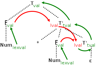
The diagram on the right illustrates a great deal.
The black dotted lines comprise the parse tree for the
multiplication grammar just studied when applied to a single
multiplication, e.g. 3*5.
Each synthesized attribute is shown in green and is
written to the right of the grammar symbol at the node where it
appears in the annotated parse tree.
This is also the node corresponding to the semantic rule calculating
the value.
Each inherited attribute is shown in red and is written to
the left of its grammar symbol at the node where it appears in the
annotated parse tree.
Note that this value is calculated by a semantic rule
at the parent of this node.
Each green arrow points to the synthesized attribute
calculated from the attribute at the tail of the arrow.
These arrows either go up the tree one level or stay at a node.
That is because a synthesized attribute can depend only on the node
where it is defined and that node's children.
The computation of the attribute is associated with the production
at the node at its arrowhead.
In this example, each synthesized attribute depends on only one
other attribute, but that is not required.
Each red arrow points to the inherited attribute
calculated from the attribute at the tail.
Note that, at the lower right T' node, two red arrows point to the
same attribute.
This indicates that the common attribute at the arrowheads, depends
on both attributes at the tails.
According to the rules for inherited attributes, these arrows either
go down the tree one level, go from a node to a sibling, or stay
within a node.
The computation of the attribute is associated with the production
at the parent of the node at the arrowhead.
5.2.2: Ordering the Evaluation of Attributes
The graph just drawn is called the dependency graph.
In addition to being generally useful in recording the relations
between attributes, it shows the evaluation order(s) that can be
used.
Since the attribute at the head of an arrow depends on the on the
one at the tail, we must evaluate the head attribute
after evaluating the tail attribute.
Thus what we need is to find an evaluation order respecting the
arrows.
This is called a topological sort.
The rule is that the needed ordering can be found if and only if
there are no (directed) cycles.
The algorithm is simple.
- Choose a node having no incoming edges
- Delete the node and all outgoing edges.
- Repeat
If the algorithm terminates with nodes remaining, there is a
directed cycle within these remaining nodes and hence no suitable
evaluation order.
If the algorithm succeeds in deleting all the nodes, then the
deletion order is a suitable evaluation order and there were no
directed cycles.
The topological sort algorithm is non-deterministic
(Choose a node) and hence there can be many
topological sort orders.
Homework: 1.
5.2.3: S-Attributed Definitions
Given an SDD and a parse tree, performing a topological sort
constructs a suitable evaluation order or announces that no such
order exists.
However, it is very difficult to determine, given
just an SDD, whether no parse
trees have cycles in their dependency graphs.
That is, it is very difficult to determine if there are suitable
evaluation orders for all parse trees.
Fortunately, there are classes of SDDs for which a suitable
evaluation order is guaranteed, and which are adequate for our
needs.
As mentioned above an SDD is S-attributed if every attribute is
synthesized.
For these SDDs all attributes are calculated from attribute values
at the children since the other possibility, the tail attribute is
at the same node, is impossible since the tail attribute must be
inherited for such arrows.
Thus no cycles are possible and the attributes can be evaluated by a
postorder traversal of the parse tree.
Since postorder corresponds to the actions of an LR parser when
reducing the body of a production to its head, it is often
convenient to evaluate synthesized attributes during an LR parse.
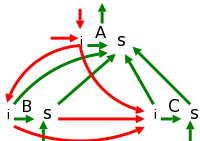
5.2.4 L-Attributed Definitions
Unfortunately, it is hard to live without inherited attributes.
For example, we need them for top-down parsing of expressions.
Fortunately, our needs can be met by a class of SDDs called
L-Attributed definitions for which we can easily find an evaluation
order.
Definition:
An SDD is
L-Attributed if each attribute is either
- Synthesized.
- Inherited
from the left
, and hence the name L-attributed.
Specifically, if the production is
A → X1X2...Xn,
then the inherited attributes for Xj can depend
only on
- Inherited attributes of A, the LHS.
- Any attribute of X1, ..., Xj-1,
i.e. only on symbols to the left of Xj.
- Attributes of Xj, *BUT* you must
guarantee (separately) that the attributes of
Xj do not by themselves cause a cycle.
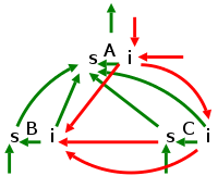
Case 2c must be handled specially whenever it occurs.
We will try to avoid it.
The top picture to the right illustrates the other cases and
suggests why there cannot be any cycles.
The picture immediately to the right corresponds to a fictitious
R-attributed definition.
One reason L-attributed definitions are favored over R, is the left
to right ordering in English.
See the example below on type declarations and also consider the
grammars that result from eliminating left recursion.
We shall see that the key property of L-attributed SDDs is that
they can be evaluated with two passes over the tree (an euler-tour
order) in which we evaluate the inherited attributes as we go down
the tree and the synthesized attributes as we go up.
The restrictions L-attributed SDDs place on the inherited attributes
are just enough to guarantee that when we go down we have all the
values needed for the inherited attributes of the child.
Fairly General, L-attributed SDD
| Production | Semantic Rule |
|---|
| A → B C
| B.inh = A.inh
C.ihn = A.inh - B.inh + B.syn
A.syn = A.inh * B.inh + B.syn - C.inh / C.syn |
| B → X | X.inh = something
B.syn = B.inh + X.syn |
| C → Y | Y.inh = something
C.syn = C.inh + Y.syn |
Evaluating L-Attributed Definitions
The table on the right shows a very simple grammar with fairly
general, L-attributed semantic rules attached.
Compare the dependencies with the general case shown in the
(red-green) picture of L-attributed SDDs above.
The picture below the table shows the parse tree for the grammar in
the table.
The triangles below B and C represent the parse tree for X and Y.
The dotted and numbered arrow in the picture illustrates the
evaluation order for the attributes; it will be discussed shortly.
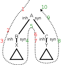
The rules for calculating A.syn, B.inh, and C.inh are shown in the
table.
The attribute A.inh would have been set by
the parent of A in the tree; the semantic rule
generating A.inh would be given with the production at the parent.
The attributes X.syn and Y.syn are calculated at the children of B
and C respectively.
X.syn can depend of X.inh and on values in the triangle below X;
similarly for Y.syn.
The picture to the right shows
that there is an evaluation
order for L-attributed definitions (again assuming no case 2c).
We just need to follow the (Euler-tour) arrow and stop at all the
numbered points.
As in the pictures above, red signifies inherited attributes and
green synthetic.
Specifically, the evaluations at the numbered stops are
- A is invoked (viewing the traversal as a program) and is
passed its inherited attributes (A.inh in our case, but of
course there could be several such attributes), which have been
evaluated at its parent.
- B is invoked by A and is given B.inh, which A has
calculated.
In programming terms: A executes
call B(B.inh)
where the argument has been evaluated by A.
This argument can depend on A.inh since the parent of A has
given A this value.
- B calls its first child (in our example X is the only
child) and passes to the child the child's inherited attributes.
In programming terms: B executes
call X(X.inh)
- The child returns, passing back to B the synthesized attributes
of the child.
In programming terms: X executes
return X.syn
In reality there could be more synthesized attributes, there
could be more children, the children could have children, etc.
- B returns to A passing back B.syn, which can depend on B.inh
(given to B by A in step 2) and X.syn
(given to B by X in the previous step).
- A calls C giving C its inherited attributes, which can depend
on A.inh (given to A, by A's parent), B.inh (previously
calculated by A in step 2), and B.syn (given to A by B in step
5).
- C calls its first child, just as B did.
- The child returns to C, just as B's child returned to B.
- C returns to A passing back C.syn, just as B did.
- A returns to its parent passing back A.syn, which can depend
on A.inh (given to A by its parent in step 1), B.inh calculated
by A in step 2, B.syn (given to A by B in step 5), C.inh
(calculated by A in step 6), and C.syn (given to A by C in step 9).
More formally, do a depth first traversal of the tree and evaluate
inherited attributes on the way down and synthetic attributes on the
way up.
This corresponds to a an Euler-tour traversal.
It also corresponds to a call graph of a program where actions are
taken at each call and each return
The first time you traverse an edge visit a node (on the way down),
evaluate its inherited attributes (in programming terms, the parent
evaluates the inherited attributes of the children and passes them
as arguments to the call).
The second time you traverse an edge and leave node (on the way back
up), you evaluate the synthesized attributes (in programming terms
the child returns the value to the parent).
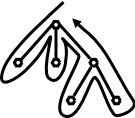
The key point is that all attributes needed will have already been
evaluated.
Consider the rightmost child of the root in the diagram on the right.
- Inherited attributes (which are evaluated on the first, i.e.,
downward, pass):
An inherited attribute depends only on inherited attributes from
the parent and on (inherited or synthesized) attributes from
left siblings.
- The parent will have already been evaluated on the
downward pass before the current child so the parent's
inherited attributes will have already been evaluated.
- The left children have already had both
passes done so all their attributes will have been
evaluated.
- Synthesized attributes (which are evaluated on the second,
i.e., upward pass):
A synthesized attribute depends only on (inherited or
synthesized) attributes of its children and on its own inherited
attributes.
- The children have already had both passes so all their
attributes have been evaluated.
- The node itself has already had its first (downward) pass
so has had its inherited attributes evaluated.
Homework: 3(a-c).
5.2.5: Semantic Rules with Controlled Side Effects
| Production | Semantic Rule | Type |
|---|
| D → T L | L.type = T.type | inherited |
| T → INT | T.type = integer | synthesized |
| T → FLOAT | T.type = float | synthesized |
| L → L1 , ID
| L1.type = L.type | inherited
|
| addType(ID.entry,L.type) | synthesized, side effect |
| L → ID | addType(ID.entry,L.type) | synthesized, side effect |
When we have side effects such as printing or adding an entry to a
table we must ensure that we have not added a constraint to the
evaluation order that causes a cycle.
For example, the left-recursive SDD shown in the table on the right
propagates type information from a declaration to entries in an
identifier table.
The function addType adds the type information in the second
argument to the identifier table entry specified in the first
argument.
Note that the side effect, adding the type info to the table, does
not affect the evaluation order.
Draw the dependency graph on the board.
Note that the terminal ID has an attribute called entry
(given by the lexer) that gives its entry in the identifier table.
The nonterminal L can be considered to have (in addition to the
inherited attribute L.type)
a dummy synthesized attribute, say AddType, that is a place holder
for the addType() routine.
AddType depends on the arguments of addType().
Since the first argument is from a child, and the second is an
inherited attribute of this node, we have legal dependences for a
synthesized attribute.
Thus we have an L-attributed definition.
Homework: For the SDD above, give the annotated
parse tree for
INT a,b,c
Start Lecture #9
5.3: Applications of Syntax-Directed Translations
5.3.1: Construction of Syntax Trees
| Production | Semantic Rules |
|---|
| E → E 1 + T
| E.node = new Node('+',E1.node,T.node) |
| E → E 1 - T
| E.node = new Node('-',E1.node,T.node) |
| E → T | E.node = T.node |
| T → ( E ) | T.node = E.node |
| T → ID | T.node = new Leaf(ID,ID.entry) |
| T → NUM | T.node = new Leaf(NUM,NUM.val) |
Recall that a syntax tree (technically
an abstract syntax tree) contains just the essential nodes.
For example, 7+3*5 would have one + node, one *, and the three
numbers.
Lets see how to construct the syntax tree from an SDD.
Assume we have two functions Leaf(op,val) and Node(op,c1,...,cn),
that create leaves and interior nodes respectively of the syntax
tree.
Leaf is called for terminals..
Op is the label of the node (op for operation) and val is the
lexical value of the token.
Node is called for nonterminals and the ci's are pointers to the
children.
| Production | Semantic Rules | Type |
|---|
| E → T E' | E.node=E'.syn | Synthesized |
| E'node=T.node | Inherited |
| E' → + T E'1
| E'1.node=new Node('+',E'.node,T.node) | Inherited |
| E'.syn=E'1.syn | Synthesized |
| E' → - T E'1
| E'1.node=new Node('-',E'.node,T.node) | Inherited |
| E'.syn=E'1.syn | Synthesized |
| E' → ε | E'.syn=E'.node | Synthesized |
| T → ( E ) | T.node=E.node | Synthesized |
| T → ID | T.node=new Leaf(ID,ID.entry) | Synthesized |
| T → NUM | T.node=new Leaf(NUM,NUM.val) | Synthesized |
The upper table on the right shows a left-recursive grammar that is
S-attributed (so all attributes are synthesized).
Try this for x-2+y and see that we get the syntax tree.
When we eliminate the left recursion, we get the lower table on the
right.
It is a good illustration of dependencies.
Follow it through and see that you get the same syntax tree as for
the left-recursive version.
Remarks:
- You probably did/are-doing/will-do some variant of new Node
and new Leaf for lab 3.
When processing a production
- Create a parse tree node for the LHS.
- Call subroutines for RHS symbols and connect the resulting
nodes to the node created in i.
- Return a reference to the new node so the parent can hook
it into the parse tree.
- It is the lack of a call to new in the third and fourth
productions (of the first, left recursive, grammar) that causes
the (abstract) syntax tree to be produced rather than the parse
(concrete syntax) tree.
- Production compilers do not produce a parse trees; rather they
produce syntax trees.
The syntax tree is smaller, and hence more (space and time)
efficient for subsequent passes that walk the tree.
The parse tree is (I believe) slightly easier to construct as
you don't have to decide which nodes to produce; you simply
produce them all.
- We could, but will not, have a lab 3.5 that takes in the parse
tree generated by lab 3 and produces an abstract syntax tree
using an SDD as illustrated by the table above.
5.3.2: The Structure of a Type
This course emphasizes top-down parsing (at least for the labs) and
hence we must eliminate left recursion.
The resulting grammars often need inherited attributes, since
operations and operands are in different productions.
But sometimes the language itself demands inherited attributes.
Consider two ways to declare a 3x4, two-dimensional array.
(Strictly speaking, these are one-dimensional arrays of
one-dimensional arrays.)
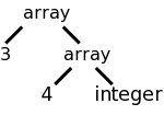
array [3] of array [4] of int and int[3][4]
Assume that we want to produce a tree structure like the one the
right for either of the array declarations on the left.
The tree structure is generated by calling a function
array(num,type).
Our job is to create an SDD so that the function gets called with
the correct arguments.
| Production | Semantic Rule |
|---|
| A → ARRAY [ NUM ] OF A1
| A.t=array(NUM.val,A1.t) |
| A → INT | A.t=integer |
| A → REAL | A.t=real |
For the first language representation of arrays (found in Ada and
in lab 3), it is easy to generate an S-attributed
(non-left-recursive) grammar based on
A → ARRAY [ NUM ] OF A | INT | REAL
This is shown in the upper table on the right.
On the board draw the parse tree and see that simple synthesized
attributes above suffice.
| Production | Semantic Rules |
|---|
| T → B C | T.t=C.t |
| C.b=B.t |
| B → INT | B.t=integer |
| B → REAL | B.t=real |
| C → [ NUM ] C1
| C.t=array(NUM.val,C1.t) |
| C1.b=C.b |
| C → ε | C.t=C.b |
For the second language representation of arrays (the
C-style), we need some smarts (and some inherited attributes) to
move the int all the way to the right.
Fortunately, the result, shown in the table on the right, is
L-attributed and therefore all is well.
Note that, instead of a third column stating whether the attribute
is synthesized or inherited, I have adopted the convention of
drawing the inherited attribute definitions with a pink background.
Also note that this is not necessary.
That is, one can look at a production and the associated semantic
rule and determine if the attribute is inherited or synthesized.
How is this done?
Answer: If the attribute being defined (i.e., the one on the LHS of
the semantic rule) is associated with the nonterminal on the LHS of
the production, the attribute is synthesized.
If the attribute being defined is associated with a nonterminal on
the RHS of the production, the attribute is inherited.
Homework: 1.
5.4: Syntax-Directed Translation Schemes (SDTs)
Basically skipped.
The idea is that instead of the SDD approach, which requires that
we build a parse tree and then perform the semantic rules in an
order determined by the dependency graph, we can attach semantic
actions to the grammar (as in chapter 2) and perform these actions
during parsing, thus saving the construction of the parse tree.
But except for very simple languages, the tree cannot be eliminated.
Modern commercial quality compilers all make multiple passes over
the tree, which is actually the syntax tree (technically, the
abstract syntax tree) rather than the parse tree (the concrete
syntax tree).
5.4.1: Postfix Translation Schemes
If parsing is done bottom up and the SDD is S-attributed, one can
generate an SDT with the actions at the end (hence, postfix).
In this case the action is perform at the same time as the RHS is
reduced to the LHS.
5.4.2: Parser-Stack Implementation of Postfix SDTs
5.4.3: SDTs with Actions Inside Productions
5.4.4: Eliminating Left Recursion from SDTs
5.4.5: SDTs For L-Attributed Definitions
5.5: Implementing L-Attributed SDD's
A good summary of the available techniques.
- Build the parse tree and annotate.
Works as long as no cycles are present (guaranteed by L- or
S-attributed).
This is the method we are using in the labs.
-
Build the parse tree, add actions, and execute the actions in
preorder.
Works for any L-attributed definition.
Can add actions based on the semantic rules of the SDD.
(Since actions are leaves of the tree, I don't
see why
preorder
is relevant).
- Translate During Recursive Descent Parsing.
This is basically combining labs 3 and 4.
See below.
Production compilers often use more complicated semantic rules
than ours and make multiple passes up and down the tree,
which renders this optimization impossible.
- Generate Code on the Fly.
Also uses recursive descent, but is restrictive.
-
Implement an SDT during LL-parsing.
-
Implement an SDT during LR-parsing of an LL Language.
5.5.1: Translation During Recursive-Descent Parsing
Recall that in fully-general, recursive-descent parsing one
normally writes one procedure for each nonterminal.
Assume the SDD is L-attributed.
We are interested in using predictive parsing for LL(1) grammars
In this case we have a procedure P for each production, which is
implemented as follows.
- P is passed the inherited attributes of its LHS nonterminal.
- P defines a variable for each attribute it will calculate.
These are the inherited attributes of the nonterminals in the
RHS and the synthesized attributes of the nonterminal
constituting the LHS.
- P processes in left-to-right order each nonterminal B
appearing in the body of the production as follows.
- Calculate the inherited attributes of B.
Since the SDD is L-attributed, these attributes do not
depend on attributes for nonterminals to the right of B
(which have not yet been processed).
- Call the procedure Q associated with this use of the
nonterminal B.
Since the grammar is LL(1) and we are using predictive
parsing, we know what production with LHS B will be used
here.
- The procedure Q returns to P the synthesized attributes of
B, which may be needed by nonterminals to the right of B.
- P calculates the synthesized attributes of the nonterminal
constituting its LHS.
- P returns these synthesized attributes to its caller (which is
the procedure associated with its parent).
5.5.2: On-the-fly Code Generation
5.5.3: L-attributed SDDs and LL Parsing
5.5.4: Bottom-Up Parsing of L-Attributed SDDs
It is interesting that this bottom-up technique requires an LL
(not just LR) language.
5.A: What Is This All Used For?
Assume we have the parse tree on the right as produced, for
example, by your lab3.
(The numbers should really be a token, e.g. NUM, not the lexemes
shown.)
You now want to write the semantics analyzer, or intermediate code
generator, or lab 4.
In any of these cases you have semantic rules or actions (for lab4
it will be semantic rules) that need to be performed.
Assume the SDD or SDT is L-attributed (that is my job for lab4), so
we don't have to worry about dependence loops.
You start to write
analyze-i.e.-traverse (tree-node)
which will be initially called with tree-node=the-root.
The procedure will perform an Euler-tour traversal of the parse tree
and during its visits of the nodes, it will evaluate the relevant
semantic rules.
The visit() procedure is basically a big switch statement where the
cases correspond to evaluating the semantic rules for the different
productions in the grammar.
The tree-node is the LHS of the production and the children are the
RHS.
By first switching on the tree-node and then inspecting enough of
the children, visit() can tell which production the tree-node
corresponds to and which semantic rules to apply.
As described in 5.5.1 above, visit() has received as parameters (in
addition to tree-node), the inherited attributes of the node.
The traversal calls itself recursively, with the tree-node argument set
to the leftmost child, then calls again using the next child, etc.
Each time, the child is passed the inherited attributes.
When each child returns, it passes back its synthesized attributes.
After the last child returns, the parent returns, passing
back the synthesized attributes that were calculated.
A programming point is that, since tree-node can be any
node, traverse() and visit() must each be prepared to accept as
parameters any inherited attribute that any nonterminal can
have.
5.A.A: Variations
-
Instead of a giant switch, you could have separate routines for
each nonterminal and just switch on the productions having this
nonterminal as LHS.
In this case each routine need be prepared to accept as
parameters only all the inherited attributes that its
nonterminal can have.
-
You could have separate routines for each production and thus
each routine has as parameters exactly the inherited attributes
that this production receives.
To do this requires knowing which visit() procedure to call for
each nonterminal (child node of the tree).
For example, assume you are processing the production
B → C D
You need to know which production to call for C
(remember that C can be the LHS of many different productions).
- You could store the (number of the) production in the tree
node.
- You could peek further down the tree to determine the
production for each of your children (i.e., you look at
grandchildren).
- You could try all productions for a given nonterminal,
telling the child what production you think it is and having
the child return failure when you are wrong.
This seems too much work to me.
- etc
- If you like actions instead of rules, perform the actions where
indicated in the SDT.
- Global variable can be used (with care) instead of parameters.
- As illustrated earlier, you can call routines instead of setting
an attribute (see addType in 5.2.5).
Chapter 6: Intermediate-Code Generation
Homework: Read Chapter 6.
6.1: Variants of Syntax Trees
6.1.1: Directed Acyclic Graphs for Expressions
The difference between a syntax DAG and a syntax tree is that the
former can have undirected cycles.
DAGs are useful where there are multiple, identical portions in a
given input.
The common case of this is for expressions where there often are
common subexpressions.
For example in the expression
X + a + b + c - X + ( a + b + c )
each individual variable is a common subexpression.
But a+b+c is not since the first occurrence has the X already
added.
This is a real difference when one considers the possibility of
overflow or of loss of precision.
The easy case is
x + y * z * w - ( q + y * z * w )
where y*z*w is a common subexpression.
It is easy to find such common subexpressions.
The constructor Node() above checks if an identical
node exists before creating a new one.
So Node ('/',left,right) first checks if there is a node with op='/'
and children left and right.
If so, a reference to that node is returned; if not, a new node is
created as before.
Homework: 1.
6.1.2: The Value-Number Method for Constructing DAGS
Often one stores the tree or DAG in an array, one entry per node.
Then the array index, rather than a pointer, is used to reference a
node.
This index is called the node's value-number and the triple
<op, value-number of left, value-number of right>
is called the signature of the node.
When Node(op,left,right) needs to determine if an identical node
exists, it simply searches the table for an entry with the required
signature.
Searching an unordered array is slow; there are many better data
structures to use.
Hash tables are a good choice.
Homework: 2.
6.2: Three-Address Code
We will use three-address code, i.e., instructions of the
form op a,b,c, where op is a primitive
operator.
For example
    lshift a,b,4   // left shift b by 4 and place result in a
    add    a,b,c   // a = b + c
    a = b + c      // alternate (more natural) representation of above
If we are starting with an expression DAG (or syntax tree if less
aggressive), then transforming into 3-address code is just a
topological sort and an assignment of a 3-address operation with a
new name for the result to each interior node (the leaves already
have names and values).
A key point is that nodes in an expression dag (or tree) have at
most 2 children so three-address code is easy.
As we produce three-address code for various constructs, we may have
to generate several instructions to translate one construct.
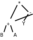
For example, (B+A)*(Y-(B+A)) produces
the DAG on the right, which yields the following 3-address code.
    t1 = B + A
    t2 = Y - t1
    t3 = t1 * t2
Notes
- We have not yet learned how to have the compiler generate the
instructions given above.
- The labs will use parse trees not syntax dags.
6.2.1: Addresses and Instructions
We use the terminology 3-address code since instructions in our
intermediate-language consist of one elementary
operation
with three operands, each of which is often an address.
Typically two of the addresses represent source operands or
arguments of the operation and the third represents the result.
Some of the 3-address operations have fewer than three addresses; we
simply think of the missing addresses as unused (or ignored) fields
in the instruction.
Possible Address Types
- (Source program) Names.
Really the intermediate code would contain a reference to the
(identifier) table entry for the name.
For convenience, the actual identifier is often written.
An important issue is type conversion, which will be discussed
later.
- Constants.
Again, this would often be a reference to a table entry.
As with names, type conversion is an important issue for constants.
- (Compiler-generated) Temporaries.
Although it may at first seem wasteful,
modern practice assigns a new name to each
temporary, rather than reusing the same temporary when possible.
(Remember that a DAG node is considered one temporary even if it
has many parents.)
Later phases can combine several temporaries into one (e.g., if
they have disjoint lifetimes).
L-values and R-values
Consider
Q := Z; or
A[f(x)+B*D] := g(B+C*h(x,y));.
Where [] indicates array reference and () indicates a function call.
From a macroscopic view, performing each assignment involves three
tasks.
- Evaluate the left hand side (LHS) to obtain an l-value.
- Evaluate the RHS to obtain an r-value.
- Perform the assignment.
Note the differences between L-values, quantities that can appear
on the LHS of an assignment, and and R-values, quantities that can
appear only on the RHS.
- An l-value corresponds to an address or a location.
- An r-value corresponds to a value.
- Neither 12 nor s+t can be used as
an l-value, but both are legal r-values.
- We say that the l-value can be dereferenced to obtain
the corresponding r-value.
Possible three-address instructions
There is no universally agreed to set of three-address
instructions, or even whether 3-address code should be the
intermediate code for the compiler.
Some prefer a set close to a machine architecture.
Others prefer a higher-level set closer to the source, for example,
subsets of C have been used.
Others prefer to have multiple levels of intermediate code in the
compiler and define a compilation phase that converts the high-level
intermediate code into the low-level intermediate code.
What follows is the set proposed in the book.
In the list below, x, y, and z are addresses; i is an integer,
not an address); and L is a symbolic label.
The instructions can be thought of as numbered and the labels can be
converted to the numbers with another pass over the output or
via backpatching
, which is discussed below.
- Binary and unary ops.
- x = y op z with op a binary operation.
- x = op y with op a unary operation.
- x = y another unary
operation, specifically the identity f(x)=x.
- Binary, unary, and nullary op jumps
- Nullary Junp.
goto L
- Conditional unary op jumps.
if x goto L
ifFalse x goto L.
- Conditional binary op jumps.
if x relop y goto L
- Procedure/Function Calls and Returns.
param x call p,n
y = call p,n
return return y.
The value n gives the number of parameters, which is needed when the
argument of one function is the value returned by another, for
example A = F(S,G(U,V),W) might become
	param S
	param U
	param V
	t = call G,2
	param t
	param W
	A = call F,3
This is not important for lab4 since we do not have functions,
and procedure calls cannot be embedded one inside the other the
way function calls can.
-
Indexed Copy ops. x = y[i] x[i] =
y.
In the second example, x[i] is the address that is
the-value-of-i locations after the address x; in particular
x[0] is the same address as x.
Similarly for y[i] in the first example.
But a crucial difference is that, since y[i] is on the RHS,
the address is dereferenced and the value in the
address is what is used.
Note that x[i] = y[j] is not permitted as that requires 4
addresses.
x[i] = y[i] could be permitted, but is not.
- Address and pointer ops. x = &y x = *y
*x = y.
x = &y sets the r-value of x equal to the l-value of y.
x = *y sets the r-value of x equal to the contents of the
location given by the r-value of y.
*x = y sets the location given by the r-value of x equal to the
r-value of y.
6.2.2: Quadruples (Quads)
Quads are an easy, almost obvious, way to represent the three
address instructions: put the op into the first of four fields and
the three addresses into the remaining three fields.
Some instructions do not use all the fields.
Many operands will be references to entries in tables (e.g., the
identifier table).
Homework: 1, 2 (you may use the parse tree instead
of the syntax tree if you prefer).
You may omit the part about triples.
6.2.3: (Indirect) Triples
Triples
A triple optimizes
a quad by eliminating the result field of
a quad since the result is often a temporary.
When this result occurs as a source operand of a subsequent
instruction, the source operand is written as the value-number of
the instruction yielding this result (distinguished some way, say
with parens).
If the result field of a quad is a program name and not a temporary
then two triples may be needed:
- Do the operation and place the result into a temporary
(which is not a field of this instruction).
- A copy instruction from the temporary to the final home.
Recall that a copy does not use all the fields of a quad so fits
into a triple without omitting the result.
Indirect Triples
When an optimizing compiler reorders instructions for increased
performance, extra work is needed with triples since the instruction
numbers, which have changed, are used implicitly.
Hence the triples must be regenerated with correct numbers as
operands.
With Indirect triples we maintain an array of pointers to
triples and, if it is necessary to reorder instructions, just
reorder these pointers.
This has two advantages.
- The pointers are (probably) smaller than the triples so faster
to move.
This is a generic advantage and could be used for quads and many
other reordering applications (e.g., sorting large records).
- Triples contain references to results computed by prior
triples.
These references are given as the number of the computing
triple.
Since, with indirect triples, the triples themselves don't move
when the instructions are reordered, the references they contain
remain accurate.
This advantage is specific to triples (or similar situations).
6.2.4: Static Single-Assignment (SSA) Form
This has become a big deal in modern optimizers, but we will
largely ignore it.
The idea is that you have all assignments go to unique (temporary)
variables.
So if the code is
if x then y=4 else y=5
it is treated as though it was
if x then y1=4 else y2=5
The interesting part comes when y is used later in the program and
the compiler must choose between y1 and y2.
6.3: Types and Declarations
Much of the early part of this section is really about programming
languages more than about compilers.
6.3.1: Type Expressions
A type expression is either a basic type or the result of applying
a type constructor.
Definition: A
type expression is one
of the following.
- A basic type.
- A type name.
- Applying an array constructor array(number,type-expression).
This is where the C/java syntax is, in my view, inferior to the
more algol-like syntax of e.g., ada and lab 3
array [ index-type ] of type.
- Applying a record constructor record(field names and types).
- Applying a function constructor type→type.
- The product type×type.
- A type expression may contain variables (that are type
expressions).
6.3.2: Type Equivalence
There are two camps, name equivalence and
structural equivalence.
Consider the following example.
    declare
       type MyInteger is new Integer;
       MyX : MyInteger;
       x   : Integer := 0;
    begin
       MyX := x;
    end
This generates a type error in Ada, which has name equivalence since
the types of x and MyX do not have the same name, although they have
the same structure.
As another example, consider an object of an anonymous
type
as in
X : array [5] of integer;
Since the type of X does not have a name,
X does not have the same type as any other object not even Y
declared as
y : array [5] of integer;
However, x[2] has the same type as y[3]; both are integers.
6.3.3: Declarations
The following example from the 2e uses an usual C/Java-like array
notation.
(The 1e had pascal-like notation.)
Although I prefer Ada-like constructs as in lab 3, I realize that
the class knows C/Java best so like the authors I will sometimes
follow the 2e as well as presenting lab3-like grammars.
I will often refer to lab3-like grammars as the class grammar.
The grammar below gives C/Java-like
records/structs/methodless-classes as well as multidimensional
arrays (really singly dimensioned arrays of singly dimensioned
arrays).
    D → T id ; D | ε
    T → B C | RECORD { D }
    B → INT | FLOAT
    C → [ NUM ] C | ε
Note that an example sentence derived from D is
int [5] x ;
which is not legal C, but does have the virtue
that the type
is separate from identifier being declared.
The class grammar doesn't support records.
This part of the class grammar declares ints, reals, arrays, and
user-defined types.
    declarations         → declaration declarations | ε
    declaration          → defining-identifier : type ; |
                           TYPE defining-identifier IS type ;
    defining-identifier  → IDENTIFIER
    type                 → INT | REAL | ARRAY [ NUMBER ] OF type | IDENTIFIER
So that the tables below are not too wide, let's use shorter names
for the nonterminals.
Specifically, we abbreviate declaration as d, declarations as ds,
defining-identifier, as di, and type as ty (unfortunately, we have
already used t to abbreviate term).
For now we ignore the second possibility for a declaration
(declaring a type itself).
    ds   → d ds | ε
    d    → di : ty ;
    di   → ID
    ty   → INT | REAL | ARRAY [ NUMBER ] OF ty
User-Defined Types
It is useful to support user-declared types.
For example
      type vector5 is array [5] of real;
      v5 : vector5;
The full class grammar does support this.
      ds   → d ds | ε
      d    → di : ty ; | TYPE di IS ty ;
      di   → ID
      ty   → INT | REAL | ARRAY [ NUMBER ] OF ty | ID
Ada Constrained vs Unconstrained Array Types
Ada supports both constrained array types such as
type t1 is array [5] of integer;
and unconstrained array types such as
type t2 is array of integer;
With the latter, the constraint is specified when the array (object)
itself is declared.
      x1 : t1
      x2 : t2[5]
You might wonder why we want the unconstrained type.
These types permit a procedure to have a parameter that is an array
of integers of unspecified size.
Remember that the declaration of a procedure specifies only the type
of the parameter; the object is determined at the time of the
procedure call.
Start Lecture #10
6.3.4: Storage Layout for Local Names
Previously we considered an SDD for
arrays that was able to compute the type.
The key point was that it called the function array(size,type) so as
to produce a tree structure exhibiting the dimensionality of the
array.
For example the tree on the right would be produced for
int[3][4]
or array [3] of array [4] of int.
Now we will extend the SDD to calculate the size of the
array as well.
For example, the array pictured has size 48, assuming that
each int has size 4.
When we declare many objects, we need to know the size of each one
in order to determine the offsets of the objects from the start of
the storage area.
We are considering here only those types for which the storage
requirements can be computed at compile time.
For others, e.g., string variables, dynamic arrays, etc, we would
only be reserving space for a pointer to the structure; the
structure itself would be created at run time.
Such structures are discussed in the next chapter.
Type and Size of Arrays
| Production | Actions | Semantic Rules |
|---|
|
|
|
| T → B | { t = B.type } | C.bt = B.bt |
| | { w = B.width } | C.bw = B.bw |
| C
| { T.type = C.type } | T.type = C.type |
| { T.width = B.width; } | T.width = C.width |
|
|
|
| B → INT | { B.type = integer; B.width = 4; }
| B.bt = integer
B.bw = 4
|
|
|
|
| B → FLOAT | { B.type = float; B.width = 8; }
| B.bt = float
B.bw = 8
|
|
|
|
| C → [ NUM ] C1
|
| C.type = array(NUM.value, C1.type)
|
|
| C.width = NUM.value * C1.width;
|
| { C.type = array(NUM.value, C1.type);
| C1.bt = C.bt
|
| C.width = NUM.value * C1.width; }
| C1.bw = C.bw
|
|
|
|
| C → ε | { C.type = t; C.width=w }
| C.type = C.bt
C.width = C.bw
|
The idea (for arrays whose size can be determined at compile time)
is that the basic type determines the width of the object, and the
number of elements in the array determines the height
.
These are then multiplied to get the size (area) of the object.
The terminology actually used is that the basetype determines the
basewidth, which when multiplied by the number of elements gives the
width.
The book uses semantic actions, i.e., a syntax directed translation
or SDT.
I added the corresponding semantic rules so that the table to the
right is an SDD as well.
In both cases we follow the book and show a single type
specification T rather than a list of object declarations D.
The omitted productions are
D → T ID ; D | ε
The goal of the SDD is to calculate two attributes of the start
symbol T, namely T.type and T.width, the rules can be viewed as the
implementation.
The basetype and hence the basewidth are determined by B, which is
INT or FLOAT.
The values are set by the lexer (as attributes of FLOAT and INT) or,
as shown in the table, are constants in the parser.
NUM.value is set by the lexer.
These attributes of B pushed down the tree via the inherited
attributes C.bw and C.bw until all the array dimensions have been
passed over and the ε-production is reached.
There they are turned around
as usual and sent back up,
during which the dimensions are processed and the final type and
width are calculated.
An alternative implementation, using global variables, is described
in the grayed out description of the semantic actions
This is similar to the comment above that instead of having the
identifier table passed up and down via attributes, the bullet can
be bitten and a globally visible table used instead.
Remember that for an SDT, the placement of the actions within the
production is important.
Since it aids reading to have the actions lined up in a column, we
sometimes write the production itself on multiple lines.
For example the production T→BC in the table below has the B
and C on separate lines so that (the first two) actions can be in
between even though they are written to the right.
These two actions are performed after the B child has been
traversed, but before the C child has been traversed.
The final two actions are at the very end so are done after both
children have been traversed.
The actions use global variables t and w to carry the base type
(INT or FLOAT) and width down to the ε-production, where
they are then sent on their way up and become multiplied by the
various dimensions.
Using the Class Grammar
Lab 3 SDD for Declarations
| Production |
Semantic Rules
(All Attributes Synthesized)
|
| d → di : ty ; |
addType(di.entry, ty.type);
addSize(di.entry, ty.size)
|
| di → ID | di.entry = ID.entry
|
| ty → ARRAY [ NUM ] OF ty1 ; |
ty.type = array(NUM.value, ty1.type)
ty.size = NUM.value * ty1.size |
| ty → INT |
ty.type = integer
ty.size = 4 |
| ty → REAL |
ty.type = real
ty.size = 8 |
This exercise is easier with the class grammar since there are no
inherited attributes.
We again assume that the lexer has defined NUM.value (it is likely a
field in the numbers table entry for the token NUM).
The goal is to augment the identifier table entry for ID to include
the type and size information found in the declaration.
This can be written two ways.
- addType(ID.entry,ty.type)
addSize(ID.entry,ty.size)
- ID.entry.type=ty.type
ID.entry.size=ty.size
The two notations mean the same thing, namely the type component of
the identifier table entry for ID is set to t.type (and similarly
for size).
It is common to write it the first way.
(In the table ID.entry is di.entry, but they are equal.)
Recall that addType is viewed as synthesized since its parameters
come from the RHS, i.e., from children of this node.
addType has a side effect (it modifies the identifier table) so we
must ensure that we do not use this table value before it is
calculated.
When do we use this value?
Answer: When we evaluate expressions, we will need to look up the
types of objects.
How can we ensure that the type has already been determined and
saved?
Answer: We will need to enforce declaration before use
.
So, in expression evaluation, we should check the entry in the
identifier table to be sure that the type has already been set.
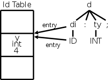
Example 1:
As a simple example, let us construct,
on the board, the parse tree for the scalar declaration
y : int ;
We get the diagram at the right, in which I have also shown the
effects of the semantic rules.
Note specifically the effect of the addType and addSize functions
on the identifier table.
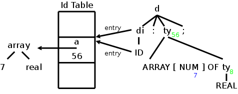
Example 2:
For our next example we choose the array declaration
a : array [7] of int ;
The result is again shown on the right.
The green numbers show the value of t.size and the blue number shows
the value of NUM.value.
Example 3:
For our final example in this section we combine the two previous
declarations into the following simple complete program.
In this example we show only the parse tree.
In the next section we consider the semantic actions as well.
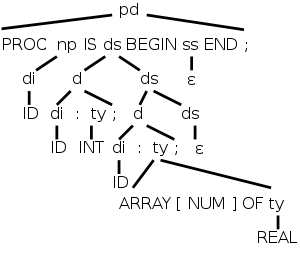
    Procedure P1 is
      y : int;
      a : array [7] of real;
    begin
    end;
We observe several points about this example.
- Since we have 2 declarations, we need to use the two
productions involving the nonterminal declarations (ds)
ds → d ds | ε
- An Euler-tree traversal of the tree will visit the
declarations before visiting any statements (I know this example
doesn't have any statements).
Thus, if we are processing a statement and find an undeclared
variable, we can signal an error since we know that there is no
chance we will visit the declaration later.
- With multiple declarations, it will be necessary to determine
the offset of each declared object.
- We will study an extension of this example in the next
section.
In particular, we will show the annotated parse tree, including
calculations of the offset just mentioned.
6.3.5: Sequences of Declarations
Remark: Be careful to distinguish between three
methods used to store and pass information.
- Attributes.
These are variables in a phase of the compiler
(the semantic analyzer a.k.a intermediate code generator).
- Identifier (and other) table.
This holds longer lived data; often passed between phases.
- Run time storage.
This is storage established by the compiler,
but not used by the compiler.
It is allocated and used during run time.
To summarize, the identifier table (and other tables we have used)
are not present when the program is run.
But there must be run time storage for objects.
In addition to allocating the storage (a subject discussed next
chapter), we need to determine the address each object will have
during execution.
Specifically, we need to know its offset from the start of the area
used for object storage.
For just one object, it is trivial: the offset is zero.
When there are multiple objects, we need to keep a running sum of the
sizes of the preceding objects, which is our next objective.
Multiple Declarations
The goal is to permit multiple declarations in the same
procedure (or program or function).
For C/java like languages this can occur in two ways.
- Multiple objects in a single declaration.
- Multiple declarations in a single procedure.
In either case we need to associate with each object being declared
the location in which it will be stored at run time.
Specifically we include in the table entry for the object, its
offset from the beginning of the current procedure.
We initialize this offset at the beginning of the procedure and
increment it after each object declaration.
The lab3 grammar does not support multiple objects in a single
declaration.
C/Java does permit multiple objects in a single declaration, but
surprisingly the 2e grammar does not.
Naturally, the way to permit multiple declarations is to have a
list of declarations in the natural right-recursive way.
The 2e C/Java grammar has D which is a list of semicolon-separated
T ID's
D → T ID ; D | ε
The lab 3 grammar has a list of declarations
(each of which ends in a semicolon).
Shortening declarations to ds we have
ds → d ds | ε
Multiple declarations snippet
| Production | Semantic Action |
|---|
|
|
| P → | { offset = 0; } |
| D | |
|
|
| D → T ID ; | { top.put(id.lexeme, T.type, offset); |
| | offset = offset + T. width; } |
| D1 |
|
|
| D → ε | |
As mentioned, we need to maintain an offset, the next storage
location to be used by an object declaration.
The 2e snippet on the right introduces a nonterminal P for program
that gives a convenient place to initialize offset.
The name top is used to signify that we work with the top symbol
table (when we have nested scopes for record definitions, nested
procedures, or nested blocks we need a stack of symbol tables).
Top.put places the identifier into this table with its type and
storage location and then bumps offset for the next variable or next
declaration.
Rather than figure out how to put this snippet together with the
previous 2e code that handled arrays, we will just present the
snippets and put everything together on the class grammar.
Multiple Declarations in the Class Grammar
Multiple Declarations
| Production | Semantic Rules |
|---|
| pd → PROC np IS ds BEG ss END ;
| ds.offset = 0
|
| ds → d ds1
|
d.offset = ds.offset
ds1.offset = d.newoffset
ds.totalSize = ds1.totalSize
|
| ds → ε
| ds.totalSize = ds.offset
|
| d → di : ty ;
| addType(di.entry, ty.type)
addSize(di.entry, ty.size)
addOffset(di.entry, d.offset)
d.newoffset = d.offset + ty.size
|
| di → ID
| di.entry = ID.entry
|
| ty → ARRAY [ NUM ] OF ty1
|
ty.type = array(NUM.value, t1.type)
ty.size = NUM.value * t1.size |
| ty → INT
|
ty.type = integer
ty.size = 4
|
| ty → REAL
|
ty.type = real
ty.size = 8
|
On the right we show the part of the SDD used to translate multiple
declarations for the class grammar.
We do not show the productions for name-and-parameters (np) or
statements (ss) since we are focusing on just the declaration of
local variables.
The new part is determining the offset for each individual
declaration.
The new items have blue backgrounds (this includes new, inherited
attributes, which were red).
The idea is that the first declaration has offset 0 and the next
offset is the current offset plus the current size.
Specifically, we proceed as follows.
In the procedure-def (pd) production, we give
the nonterminal declarations
(ds) the inherited attribute
offset (ds.offset), which we initialize to zero.
We inherit this offset down to individual declarations.
At each declaration (d), we store the offset in the entry for the
identifier being declared and increment the offset by the size of
this object.
When we get the to the end of the declarations (the
ε-production), the offset value is the total size needed.
We turn it around and send it back up the tree in case the total
is needed by some higher level production.
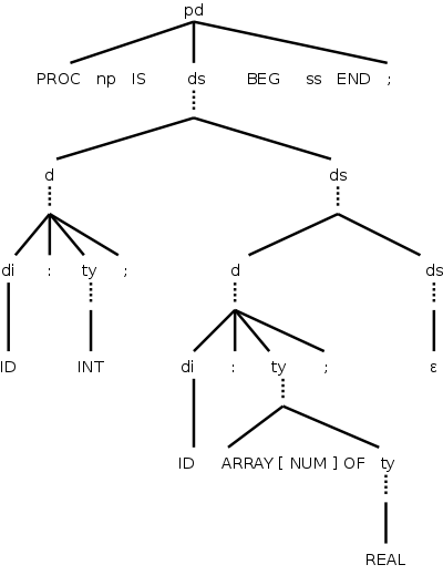
Example: What happens when the following program
(an extension of P1 from the previous section) is parsed and the
semantic rules above are applied.
  procedure P2 is
      y : integer;
      a : array [7] of real;
  begin
      y := 5;      // Statements not yet done
      a[2] := y;   // Type error?
  end;
On the right is the parse tree, limited to the declarations.
The dotted lines would be solid for a parse tree and connect to the
lines below.
They are shown dotted so that the figure can be compared to the
annotated parse tree immediately below, in which the attributes and
their values have been filled in.
In the annotated tree, the attributes shown in red are inherited.
Those in black are synthesized.
To start the annotation process, look at the top production in the
parse tree.
It has an inherited attributed ds.offset, which is set to zero.
Since the attribute is inherited, the entry can be placed
immediately into the annotated tree.
We now do the left child and fill in its inherited attribute.
When the Euler tour comes back up the tree, the synthesized
attributes are evaluated and recorded.
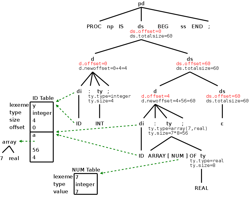
6.3.6: Fields in Records and Classes
Since records can essentially have a bunch of declarations inside,
we only need add
T → RECORD { D }
to get the syntax right.
For the semantics we need to push the environment and offset onto
stacks since the namespace inside a record is distinct from that on
the outside.
The width of the record itself is the final value of (the inner)
offset, which in turn is the value of totalsize at the root when the
inner scope is concluded.
  T → record {  { Env.push(top);
                  top = new Env();
                  Stack.push(offset);
                  offset = 0; }
  D }           { T.type = record(top);
                  T.width = offset;
                  top = Env.pop();
                  offset = Stack.pop(); }
This does not apply directly to the class grammar, which does not
have records.
This same technique would be used for other examples of nested
scope, e.g., nested procedures/functions and nested blocks.
To have nested procedures/functions, we need other alternatives for
declaration: procedure/function definitions.
Similarly if we wanted to have nested blocks we would add another
alternative to statement.
  s           → ks | ids | block-stmt
  block-stmt  → DECLARE ds BEGIN ss END ;
If we wanted to generate code for nested procedures or nested
blocks, we would need to stack the symbol table as done above and in
the text.
Homework: 1.
6.4: Translation of Expressions
Scalar Expressions
| Production | Semantic Rule |
|---|
| e → t
|
e.addr = t.addr
e.code = t.code
|
| e → e1 ADDOP t
|
e.addr = new Temp()
e.code = e1.code || t.code ||
gen(e.addr = e1.addr ADDOP.lexeme t.addr)
|
| t → f
|
t.addr = f.addr
t.code = f.code
|
| t → t1 MULOP f
|
t.addr = new Temp()
t.code = t1.code || f.code ||
gen(t.addr = t1.addr MULOP.lexeme f.addr)
|
| f → ( e )
|
f.addr = e.addr
f.code = e.code
|
| f → NUM
|
f.addr = get(NUM.lexeme)
f.code = ""
|
| f → ID is
|
assume indices is ε
f.addr = get(ID.lexeme)
f.code = ""
|
The goal is to generate 3-address code for scalar expressions,
i.e., arrays are not treated in this section (they will be shortly).
Specifically, indices is assumed to be ε.
We use is to abbreviate indices.
We generate the 3-address code using the natural
notation of
6.2.
In fact we assume there is a function gen() that, given the pieces
needed, does the proper formatting so gen(x = y + z) will output the
corresponding 3-address code.
gen() is often called with addresses other than lexemes, e.g.,
temporaries and constants.
The constructor Temp() produces a new address in whatever format gen
needs.
Hopefully this will be clear in the table to the right and the
others that follow.
6.4.1: Operations Within Expressions
We will use two attributes code and address (addr).
The key objective at each node of the parse tree for an expression
is to produce values for the code and addr attributes so that the
following crucial invariant is maintained.
If code
is executed, then address addr
contains
the value of the (sub-)expression routed at this node.
In particular, after TheRoot.code is evaluated, the address
TheRoot.addr contains the value of the entire expression.
Said another way, the attribute addr at a node is the address that
holds the value calculated by the code at the node.
Recall that unlike real code for a real machine our 3-address code
doesn't reuse temporary addresses.
As one would expect for expressions, all the attributes in the
table to the right are synthesized.
The table is for the expression part of the class grammar.
To save space we use ID for IDENTIFIER,
e for expression, t for term, and f for factor.
The SDDs for declarations and scalar expressions can be easily
combined by essentially concatenating them as shown
here.
6.4.2: Incremental Translation
We saw this in chapter 2.
The method in the previous section generates long strings as we
walk the tree.
By using SDTs instead of SDDs, you can output parts of the string
as each node is processed.
6.4.3: Addressing Array Elements
Declarations with Basetypes
| Production | Semantic Rules |
|---|
| pd → PROC np IS ds BEG ss END ;
| ds.offset = 0
|
| np → di ( ps ) | di
| not used yet
|
| ds → d ds1
|
d.offset = ds.offset
ds1.offset = d.newoffset
|
| ds.totalSize = ds1.totalSize |
| ds → ε
| ds.totalSize = ds.offset
|
| d → di : ty ;
|
addType(di.entry, ty.type)
addBaseType(di.entry, ty.basetype)
addSize(di.entry, ty.size)
addOffset(di.entry, d.offset)
d.newoffset = d.offset + ty.size
|
| di → ID
| di.entry = ID.entry
|
| ty → ARRAY [ NUM ] OF ty1
|
ty.type = array(NUM.value, ty1.type)
ty.basetype = ty1.basetype
ty.size = NUM.value * ty1.size
|
| ty → INT
|
ty.type = integer
ty.basetype = integer
ty.size = 4
|
| ty → REAL
|
ty.type = real
ty.basetype = real
ty.size = 8
|
The idea is to associate the base address with the array name.
That is, the offset stored in the identifier table entry for the
array is the address of the first element.
When an element is referenced, the indices and the array bounds are
used to compute the amount, often called the offset (unfortunately,
we have already used that term), by which the address of the
referenced element differs from the base address.
To implement this technique, we must first store the base type of
each identifier in the identifier table.
We use this basetype to determine the size of each element of the
array.
For example, consider
    arr: array [10] of integer;
    x  : real ;
Our previous SDD for declarations calculates the size and type of
each identifier.
For arr these are 40 and array(10,integer),
respectively.
The enhanced SDD on the right calculates, in addition, the base
type.
For arr this is integer.
For a scalar, such as x, the base type is the same as the
type, which in the case of x is real.
The new material is shaded in blue.
This SDD is combined with the expression SDD
here.
One Dimensional Arrays
Calculating the address of an element of a one dimensional array is
easy.
The address increment is the width of each element times the index
(assuming indices start at 0).
So the address of A[i] is the base address of A,
which is the offset component of A's entry in the identifier table,
plus i times the width of each element of A.
The width of each element of an array is the width of what we have
called the base type of the array.
For a scalar, there is just one element and its width is the width of
the type, which is the same as the base type.
Hence, for any ID the element width is
sizeof(getBaseType(ID.entry)).
For convenience, we define getBaseWidth by the formula
getBaseWidth(ID.entry) = sizeof(getBaseType(ID.entry)) = sizeof(ID.entry.baseType)
Two Dimensional Arrays
Let us assume row major ordering.
That is, the first element stored is A[0,0], then A[0,1], ... A[0,k-1], then
A[1,0], ... .
Modern languages use row major ordering.
With the alternative column major ordering, after A[0,0]
comes A[1,0], A[2,0], ... .
For two dimensional arrays the address of A[i,j] is the sum of three terms
- The base address of A.
- The distance from A to the start of row i.
This is i times the width of a row, which is
i times the number of elements in a row times the width of an element.
The number of elements in a row is the column array
bound.
- The distance from the start of row i to element A[i,j].
This is j times the width of an element.
Remarks
- Our grammar really declares one dimensional arrays of one
dimensional arrays rather than 2D arrays.
I believe this makes it easier.
- The SDD above when processing the declaration
A : array [5] of array [9] of real;
gives A the type array(5,array(9,real)) and thus the type
component of the entry for A in the symbol table contains all
the values needed to compute the address of any given element of
the array.
End of Remarks
Higher Dimensional Arrays
The generalization to higher dimensional arrays is clear.
A Simple Example
Consider the following expression containing a simple array
reference, where a and c are integers and b is a real array.
a = b[3*c]
We want to generate code something like
    T1 = #3 * c    // i.e. mult T1,#3,c
    T2 = T1 * 8    // each b[i] is size 8
    a  = b[T2]     // Uses the x[i] special form
If we considered it too easy to use the that special form we would
generate something like
    T1 = #3 * c
    T2 = T1 * 8
    T3 = &b
    T4 = T2 + T3
    a  = *T4
One-Dimensional Array References in Expressions
| Production | Semantic Rules |
|---|
| f → ID i |
f.t1 = new Temp()
f.addr = new Temp
f.code = i.code ||
gen(f.t1 = i.addr * getBaseWidth(ID.entry)) ||
gen(f.addr = get(ID.lexeme)[f.t1])
|
| f → ID i |
f.t1 = new Temp()
f.t2 = new Temp()
f.t3 = new Temp()
f.addr = new Temp
f.code = i.code ||
gen(f.t1 = in.addr * getBaseWidth(ID.entry)) ||
gen(f.t2 = &get(ID.lexeme)) ||
gen(f.t3 = f.t2 + f.t1) || gen(f.addr = *f.t3)
|
| i → [ e ]
|
i.addr = e.addr
i.code = e.code
|
6.4.4: Translation of Array References (Within Expressions)
To permit arrays in expressions, we need to specify the semantic
actions for the production
factor → IDENTIFIER indices
One-Dimensional Array References
As a warm-up, lets start with references to one-dimensional arrays.
That is, instead of the above production, we consider the simpler
factor → IDENTIFIER index
The table on the right does this in two ways, both with and without
using the special addressing form x[j].
In the table the nonterminal index is abbreviated i .
I included the version without the x[j] special form for two
reasons.
- Since we are restricted to one dimensional arrays, the full
code generation for the address of an element is not
hard.
- I thought it would be instructive to see the full address
generation without hiding some of it under the covers.
It was definitely instructive for me!
Note that by avoiding the special form b=x[j], I ended up
using two other special forms.
Is it possible to avoid the special forms?
An Aside on Special Forms: An Example From Lisp
Lisp is taught in our programming languages course, which
is a prerequisite for compilers.
If you no longer remember Lisp, don't worry.
- In Lisp there is a simple evaluation rule.
To evaluate, for example, (a b c d) you
- Evaluate all four components.
- Confirm that the first component evaluates to a
function.
- Invoke this function passing as arguments the values
calculated for the other three components.
- But this rule is not always applied!
- Instead there are
special forms
that are evaluated
differently.
- For example (setq x y) does not evaluate x prior to invoking
setq.
Our Special Forms for Addressing
We just (optionally) saw an exception to the basic lisp evaluation
rule.
A similar exception occurs with x[j] in our three-address
code.
It is a special form
in that, unlike the normal rules for
three-address code, we don't use the address
of j but instead its value.
Specifically the value of j is added to
the address of x.
The rules for addresses in 3-address code also include
    a = &b
    a = *b
    *a = b
which are other special forms
.
They have the same meaning as in the C programming language.
Incorporating 1D Arrays in the Expression SDD
Our current
SDD includes the production
f → ID is
with the added assumption that indices is ε.
We now want to permit indices to be a single index as well as
ε.
That is we replace the above production with the pair
    f → ID
    f → ID i
The semantic rules for each case were given in previous tables.
The ensemble to date is given
here.
On the board evaluate e.code for the RHS of the simple example
above: a=b[3*c].
This is an exciting moment.
At long last we really seem to be compiling!
Multidimensional Array References
As mentioned above in the general case we must process the
production
f → IDENTIFIER is
Following the method used in the 1D case we need to
construct is.code.
The basic idea is shown
here
The Left-Hand Side
Now that we can evaluate expressions (including one-dimensional
array reverences) we need to handle the left-hand side of an
assignment statement (which also can be an array reference).
Specifically we need semantic actions for the following productions
from the class grammar.
    id-statement   → ID rest-of-either
    rest-of-either → rest-of-assignment
    rest-of-assignment → := expression ;
    rest-of-assignment → indices := expression
Scalars and One Dimensional Arrays on the Left Hand Side
Assignment Statements
| Production | Semantic Rules |
|---|
| ss → s ss1
| ss.code = s.code || ss1.code
|
| ss → ε
| ss.code = ""
|
| s → ids
| s.code = ids.code
|
| ids → IDENTIFIER re
|
re.id = IDENTIFIER.entry
ids.code = re.code
|
| re → ra
| ra.id = re.id
re.code = ra.code
|
| ra → := e ; |
ra.code = e.code ||
gen(ra.id.lexeme=e.addr) |
| ra → i := e ; |
ra.t1 = newTemp()
ra.code = i.code || e.code ||
gen(ra.t1 = i.addr * getBaseWidth(ra.id)||
gen(ra.id.lexeme[ra.t1]=e.addr)
|
Once again we begin by restricting ourselves to one-dimensional
arrays, which corresponds to replacing indices
by index in the last production.
The SDD for this restricted case is shown on the right.
The first three productions reduce statements (ss) and statement
(s) to identifier-statement (ids), which is used for statements such
as assignment and procedure invocation, that begin with an
identifier.
The corresponding semantic rules simply concatenate all the code
produced into the top ss.code.
The identifier-statement production captures the ID and sends it
down to the appropriate rest-of-assignment (ra) production where the
necessary code is generated and passed back up.
The simple ra → := e; production generates ra.code by
simply appending to the evaluation of the RHS, the natural
assignment with ra as the LHS.
It is instructive to compare ra.code for the
ra → i := e production with f.code for the f → ID
i production in the expression SDD.
Both compute the same offset (index*elementSize) and both use a
special form for the address x[j]=y in this section, and y=x[j] for
expressions.
Incorporating these productions and semantic rules gives
this SDD.
Note that we have added a semantic rule to the procedure-def (pd)
production that simply sends ss.code to pd.code so that we have
obtained the overall goal setting pd.code to the entire code needed
for the procedure.
Multi-dimensional Arrays on the Left Hand Side
The idea is the same as when a multidimensional array appears in an
expression.
Specifically,
- Traverse the sub-tree routed at the top indices node and
compute the total offset from the start of the array.
- Multiply this offset by the width of each entry.
- A[product] = RHS
Our Simple Example Revisited
Recall the program we could partially
handle.
  procedure P2 is
      y : integer;
      a : array [7] of real;
  begin
      y := 5;      // Statements not yet done
      a[2] := y;   // Type error?
  end;
Now we can do the statements.
Homework: What code is generated for
the program written above?
Please remind me to go over this homework next class.
What should we do about the possible type error?
- We could ignore errors.
- We could assume the intermediate language permits mismatched
types.
Final code generation would then need to generate conversion
code or signal an error.
- We could change the program to use only one type.
- We could learn about type checking and conversions.
Let's take the last option.
Start Lecture #11
6.5: Type Checking
Type Checking includes several aspects.
- The language comes with a
type system, i.e., a set of rules saying what
types can appear where.
- The compiler assigns type expressions to parts of the source
program.
- The compiler ensures that the type usage in the program
conforms to the type system for the language.
This does not mean that the necessary type checks are performed
at compile time.
For any language, all type checking could be done at run time,
i.e. there would be no compile-time checking.
However, that does not mean the compiler is absolved from the type
checking.
Instead, the compiler generates code to do the checks at run time.
It is normally preferable to perform the checks at compile time, if
possible.
Some languages have very weak typing; for example, variables can
change their type during execution.
Often these languages need run-time checks.
Examples include lisp, snobol, and apl.
A sound type system guarantees that all checks can
be performed prior to execution.
This does not mean that a given compiler will make all the necessary
checks.
An implementation is strongly typed if
compiled programs are guaranteed to run without type errors.
6.5.1: Rules for Type Checking
There are two forms of type checking.
- We will learn type synthesis where the types
of parts are used to infer the type of the whole.
For example, integer+real=real.
- Type inference is very slick.
The type of a construct is determined from its usage.
This permits languages like ML to check types even though
names need not be declared.
We will implement type checking for expressions.
Type checking statements is similar.
The SDDs below (and for lab 4) contain type checking (and coercions)
for assignment statements as well as expressions.
6.5.2: Type Conversions
A very strict type system would do no automatic conversion.
Instead it would offer functions for the programmer
to explicitly convert between selected types.
With such a system, either the program has compatible types or is in
error.
Such explicit conversions supplied by the programmer are
called casts.
We, however, will consider a more liberal approach in which the
language permits certain implicit conversions that the
compiler is to supply.
This is called type coercion.
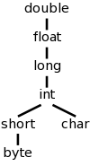
We continue to work primarily with the two basic types integer and
real, and postulate a unary function denoted (real) that converts an
integer into the real having the same value.
Nonetheless, we do consider the more general case where there are
multiple types some of which have coercions (often called
widenings).
For example in C/Java, int can be widened to long, which in turn can
be widened to float as shown in the figure to the right.
Mathematically the hierarchy on the right is a partially order set
(poset) in which each pair of elements has a least upper bound (LUB).
For many binary operators (all the arithmetic ones we are
considering, but not exponentiation) the two operands are converted
to the LUB.
So adding a short to a char, requires both to be converted to an
int.
Adding a byte to a float, requires the byte to be converted to a
float (the float remains a float and is not converted).
Checking and Coercing Types for Basic Arithmetic
The steps for addition, subtraction, multiplication, and division
are all essentially the same:
- Determine the result type, which is the LUB of the two operand
types.
- Convert each operand to the result type.
This step may require generating code or may be a no op.
- Perform the arithmetic on the converted types.
Two functions are convenient.
- LUB(t1,t2) returns the type that is the LUB of the two given
types.
It signals an error if there is no LUB, for example if one of the
types is an array.
- widen(A,T,W,newcode,newaddr).
Given an address A of type T, and a wider (or equally wide)
type W, produce newcode, the instructions needed so that the
address newaddr is the conversion of address A to type W.
LUB is simple, just look at the address latice.
If one of the type arguments is not in the lattice, signal an error;
otherwise find the lowest common ancestor.
For our case the lattice is trivial, real is above
int.
The widen function is more interesting.
It involves n2 cases for n types.
Many of these are error cases (e.g., if T wider than W).
Below is the code for our situation with two possible types integer
and real.
The four cases consist of 2 nops (when T=W), one error (T=real;
W=integer) and one conversion (T=integer; W=real).
    widen (A:addr, T:type, W:type, newcode:string, newaddr:addr)
      if T=W
        newcode = ""
        newaddr = A
      else if T=integer and W=real
        newaddr = new Temp()
        newcode = gen(newaddr = (real) A)
      else signal error
With these two functions it is not hard to modify the rules to catch
type errors and perform coercions for arithmetic expressions.
- Maintain the type of each operand by defining type attributes
for e, t, and f.
- Coerce each operand to the LUB.
This requires that we have type information for the base entities,
identifiers and numbers.
The lexer supplies the type of the numbers.
It is more interesting for the identifiers.
We inserted that information when we processed declarations.
So we now have another semantic check:
Is the identifier declared before it is used?
We will not explicitly perform this check.
To do so would not be hard.
The following analysis is similar to the one given in the previous
homework solution.
I repeat the explanation here because it is important to understand
the workings of SDDs.
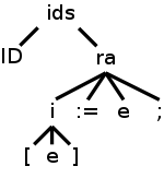
Before taking on the entire SDD, let's examine a particularly
interesting entry
identifier-statement → IDENTIFIER rest-of-assignment
and its right child
rest-of-assignment → index := expression ;
Consider the assignment statement
A[3/X+4] := X*5+Y;
the top of whose parse tree is shown on the right (again making the
simplification to one-dimensional arrays by replacing indices with
index).
Consider the ra node, i.e., the node corresponding to the
production.
ra → i := e ;
When the tree traversal gets to the ra node the first time,
its parent has passed in the value of the inherited attribute
ra.id=id.entry.
Thus the ra node has access to the identifier table entry for ID,
which in our example is the variable A.
Prior to doing its calculations, the ra node invokes its children
and gets back all the synthesized attributes.
Alternately said, when the tree traversal gets to this node
the last time, the children have returned all the
synthesized attributes.
To summarize, when the ra node finally performs its calculations, it
has available.
- ra.id: the identifier entry for A.
- i.addr/i.code: executing i.code results in i.addr containing
the value of the index, which is the expression 3/X+4.
- e.addr/e.code: executing e.code results in e.addr containing
the value of the expression X*5+Y.
- i.type/e.type: The types of the expressions.
Assignment Statements With Type Checks and Coercions
(Without Multidimensional Arrays)
| Production | Semantic Rule |
|---|
| ids → ID ra
| ra.id = ID.entry
ids.code = ra.code
|
| ra → := e ;
|
widen(e.addr, e.type, ra.id.basetype, ra.code1, ra.addr)
ra.code = e.code || ra.code1 || gen(ra.id.lexeme=ra.addr)
|
ra → i = e ;
Note: i not is
| ra.t1 = newTemp()
widen(e.addr, e.type, ra.id.basetype, ra.code1, ra.addr)
ra.code = i.code || gen(ra.t1 = getBaseWidth(ra.id)*i.addr)
|| e.code || ra.code1 ||
gen(ra.id.lexeme[ra.t1]=ra.addr)
|
| i → e
| i.addr = e.addr
i.type = e.type
i.code = e.code
|
| e → e1 ADDOP t
| e.addr = new Temp()
e.type = LUB(e1.type, t.type)
widen(e1.addr, e1.type, e.type, e.code1, e.addr1)
widen(t.addr, t.type, e.type, e.code2, e.addr2)
e.code = e1.code || e.code1 || t.code || e.code2 ||
gen(e.addr = e.addr1 ADDOP.lexeme e.addr2)
|
| e → t
| e.addr = t.addr
e.type = t.type
e.code = t.code
|
| t → t1 MULOP f
| t.addr = new Temp()
t.type = LUB(t1.type, f.type)
widen(t1.addr, t1.type, t.type, t.code1, t.addr1)
widen(f.addr, f.type, t.type, t.code2, t.addr2)
t.code = t1.code || t.code1 || f.code || t.code2 ||
gen(t.addr = t.addr1 MULOP.lexeme t.addr2)
|
| t → f
| t.addr = f.addr
t.type = f.type
t.code = f.code
|
| f → ( e )
| f.addr = e.addr
f.type = e.type
f.code = e.code
|
| f → NUM
| f.addr = NUM.lexeme
f.type = NUM.entry.type
f.code = ""
|
f → ID
(i.e., indices=ε)
|
f.addr = ID.lexeme
f.type = getBaseType(ID.entry)
f.code = ε
|
f → ID i
Note: i not is
|
f.t1 = new Temp()
f.addr = new Temp()
f.type = getBaseType(ID.entry)
f.code = i.code || gen(f.t1=i.addr*getBaseWidth(ID.entry))
|| gen(f.addr=ID.lexeme[f.t1])
|
What must the ra node do?
- Check that i.type is int (I don't do this, but
should/could).
- Ensure execution of i.code and e.code.
- Multiply i.addr by the base width of the array A.
(We need a temporary, ra.t1, to hold the computed
value).
- Widen e to the base type of A.
(We may need, and widen would then generate, a temporary
ra.addr to hold the widened value).
- Do the actual assignment of X*5+Y to A[3/X+4].
I hope the above illustration clarifies the semantic rules for
the
ra → i := e ;
production in the SDD on the right.
Because we are not considering multidimensional-arrays, the
f → ID is
production (is abbreviates indices) is replaced by the two
special cases corresponding to scalars and one-dimensional arrays,
namely:
f → ID
f → ID i
The above illustration should also help understanding the semantic
rules for this last production.
The result of incorporating these rules in our growing SDD is given
here.
Homework: Same question as the previous homework
(What code is generated for the program written above?).
But the answer is different!
Please remind me to go over the answer next class.
For lab 4, I eliminated the left recursion for expression
evaluation.
This was an instructive exercise for me, so let's do it here.
6.5.3: Overloading of Functions and Operators
Overloading is when a function or operator has several definitions
depending on the types of the operands and result.
6.5.4: Type Inference and Polymorphic Functions
6.5.5: An Algorithm for Unification
6.6: Control Flow
A key to the understand of control flow is the study of Boolean
expressions, which themselves are used in two roles.
- They can be computed and treated similar to integers and reals.
In many programming languages once can declare Boolean
variables, use the Boolean constants true and
false, and construct larger Boolean expression using
Boolean operators such as and and or.
There are also relational operators that produce Boolean values
from arithmetic operands.
From this point of view, Boolean expressions are similar to the
expressions we have already treated.
Our previous semantic rules could be modified to generate the
code needed to evaluate these expressions.
- Boolean expressions are used in certain statements that alter
the normal flow of control.
It is in this regard that we have something new to
learn.
6.6.1: Boolean Expressions
One question that comes up with Boolean expressions is whether both
operands need be evaluated.
If we are evaluating A or B and find that A is
true, must we evaluate B?
For example, consider evaluating
A=0 OR 3/A < 1.2
when A is zero.
This issue arises in other cases not involving Booleans at all.
Consider A*F(x).
If the compiler determines that A must be zero at this point, must
it generate code to evaluate F(x)?
Don't forget that functions can have side effects.
6.6.2: Short-Circuit (or Jumping) Code
Consider
    IF bool-expr-1 OR bool-expr-2 THEN
        then-clause
    ELSE
        else-clause
    END;
where bool-expr-1 and bool-expr-2 are Boolean
expressions we have already generated code for.
For a simple case think of them as Boolean variables, x and
y.
When we compile the if condition
bool-expr-1 OR bool-expr-2 we do not use
an OR operator.
Instead, we generate jumps to either the true branch or the false
branch.
We shall see that the above source code in the comparatively simple
case where bool-expr-1=x and bool-expr-2=y will
generate
    if x goto L2
    goto L4
    L4:
    if y goto L2
    goto L3
    L2:
    then-clause-code
    goto L1
    L3:
    else-clause-code
    L1:  -- This label (if-stmt.next) was defined higher in the SDD tree
Note that the compiled code does not evaluate y if
x is true.
This is the sense in which it is called short-circuit code.
As we have stated above, for many programming languages, it is
required that we not evaluate y if x is true.
6.6.3: Flow-of-Control Statements
The class grammar has the following productions concerning
flow of control statements.
    program           → procedure-def program | ε
    procedure-def     → PROCEDURE name-and-params IS decls BEGIN statement statements END ;
    statements        → statement statements | ε
    statement         → keyword-statement | identifier-statement
    keyword-statement → return-statement | while-statement | if-statement
    if-statement      → IF boolean-expression THEN statements optional-else END ;
    optional-else     → ELSE statements | ε
    while-statement   → WHILE boolean-expression DO statements END ;
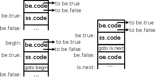
I don't show the productions for name-and-parameters, declarations,
identifier-statement, and return-statement since they do not have
conditional control flow.
The productions for boolean-expression will be done in the next section.
In this section we will produce an SDD for the productions above under
the assumption that the SDD for Boolean expressions generates jumps to the
labels be.true and be.false (depending of course on whether the
Boolean expression be is true or false).
The diagrams on the right give the idea for the three basic control
flow statements, if-then (upper left), if-then-else (right), and
while-do (lower-left).
If and While SDDs
| Production | Semantic Rules |
|---|
| pg → pd pg1
| pd.next = new Label()
pg.code = pd.code || label(pd.next) || pg1.code
|
| pg → ε | pg.code = "" |
| pd → PROC np IS ds BEG ss END ;
| pd.code = ss.code
|
| ss → s ss1
| s.next = new Label()
ss.code = s.code || label(s.next) || ss1.code
|
| ss → ε
| ss.code = ""
|
| s → ks
| ks.next = s.next
s.code = ks.code
|
| ks → ifs
| ifs.next = ks.next
ks.code = is.code
|
| ifs → IF be THEN ss oe END ;
| be.true = new Label()
be.false = new Label()
oe.next = ifs.next
ifs.code = be.code || label(be.true) || ss.code ||
gen(goto is.next) || label(be.false) || oe.code
|
| oe → ELSE ss
| oe.code = ss.code
|
| oe → ε
| oe.code = ""
|
| ks → ws
| ws.next = ks.next
ks.code = ws.code
|
| ws → WHILE be DO ss END ;
| ws.begin = new Label()
be.true = new Label()
be.false = ws.next
ss.next = ws.begin
ws.code = label(ws.begin) || be.code ||
label(be.true) || ss.code || gen(goto begin)
|
The table to the right gives the details via an SDD.
To enable the tables to fit I continue to abbreviate severely the
names of the nonterminals.
New abbreviations are ks (keyword-statement), ifs (if-statement), be
(boolean-expression), oe (optional-else) and ws (while-statement).
The remaining abbreviations, to be introduced next section, are bt
(boolean-term) and bf (boolean-factor)
The treatment of the various *.next attributes deserves some
comment.
Each statement (e.g., if-statement
abbreviated ifs or while-stmt
abbreviated ws) is given, as an inherited attribute, a new
label *.next.
You can see the new label generated in the
statements → statement statements
production and then notice how it is passed down the tree
from statements to statement
to keyword-statement to
if-statementt.
The child generates a goto *.next if it wants to end (look at
ifs.code in the if-statement production).
The parent, in addition to sending this attribute to the child,
normally places label(*.next) after the code for the child.
See ss.code in the stmts → stmt stmts production.
An alternative design would have been for the child to itself
generate the label and place it as the last component of its code
(or elsewhere if needed).
I believe that alternative would have resulted in a clearer SDD with
fewer inherited attributes.
The method actually chosen does, however, have one and possibly two
advantages.
- Perhaps there is a case where it is awkward for the child to
place something at the end of its code (but I don't quite see
how this could be).
To investigate if this second possibility occurs one might want
to examine the treatment of case statements below.
- Look at ws.code, the code attribute for the while statement.
The parent (the while-stmt) does not place the ss.next
label after ss.code.
Instead it is placed before ss.code (actually before the while
test, which is before ss.code) since right after ss.code is
an unconditional goto to the while test.
If we used the alternative where the child (the stmts)
generated the ss.next at the end of its code, the parent would
still need a goto from after ss.code to the begin label.
If the child needed to jump to its end it would jump to the
ss.next label and the next statement would be the jump to begin.
With the scheme we are using we do not have this embarrassing
jump to jump
sequence.
I must say, however, that, given all the non-optimal code we
are generating, it might have been pedagogically better to use
the alternative scheme and live with the jump to a jump
embarrassment.
I decided in the end to follow the book, but am not sure that
was the right decision.
Homework: Give the SDD for a repeat statement
REPEAT ss WHILE be END ;
Boolean Expressions
| Production | Semantic Rules |
|---|
| be → bt OR be1
| bt.true = be.true
bt.false = new Label()
be1.true = be.true
be1.false = be.false
be.code = bt.code || label(bt.false) || be1.code
|
| be → bt
| bt.true = be.true
bt.false = be.false
be.code = bt.code
|
| bt → bf AND bt1
|
bf.true = new Label()
bf.false = bt.false
bt1.true = bt.true
bt1.false = bt.false
bt.code = bf.code || label(bf.true) || bt1.code
|
| bt → bf
| bf.true = bt.true
bf.false = bt.false
bt.code = bf.code
|
| bf → NOT bf1
| bf1.true = bf.false
bf1.false = bf.true
bf.code = bf1.code
|
| bf → TRUE
| bf.code = gen(goto bf.true)
|
| bf → FALSE
| bf.code = gen(goto bf.false)
|
| bf → e RELOP e1
| bf.code = e.code || e1.code
|| gen(if e.addr RELOP.lexeme e1.addr goto bf.true)
|| gen(goto bf.false)
|
6.6.4: Control-Flow Translation of Boolean Expressions
The SDD for the evaluation of Boolean expressions is given on the
right.
All the SDDs are assembled together
here.
Recall that in evaluating the Boolean expression the objective
is not simply to produce the value true or
false, but instead, the goal is to generate a
goto be.true or a goto be.false (depending of
course on whether the Boolean expression evaluates to true
or to false).
Recall as well that we must not evaluate the right-hand
argument of an OR if the left-hand argument evaluates to
true and we must not evaluate the right-hand
argument of an AND if the left-hand argument evaluates to
true.
Notice a curiosity.
When evaluating arithmetic expressions, we needed to write
expr → expr + term
and not
expr → term + expr
in order to achieve left associativity.
But with jumping code we evaluate each factor (really
boolean-factor) in left to right order and jump out as soon as the
condition is determined.
Hence we can use the productions in the table, which conveniently
are not left recursive.
Look at the rules for the first production in the table.
If bt yields true, then we are done (i.e., we want to jump
to be.true).
Thus we set bt.true=be.true, knowing that when bt is evaluated (look
at be.code) bt will now jump to be.true.
On the other hand, if bt yields false, then we must
evaluate be1, which is why be.code has the label for
bt.false right before be1.code.
In this case the value of be is the same as the value of
be1, which explains the assignments to
be1.true and be1.false.
Do on the board the translation of
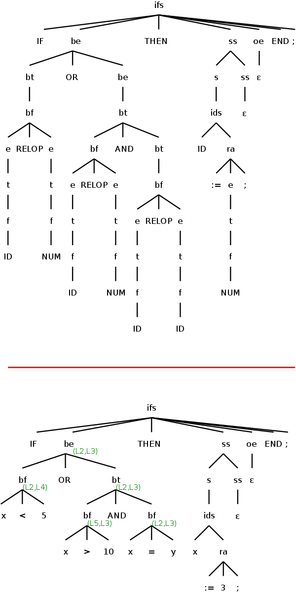
    IF   x<5  OR  x>10 AND x=y  THEN
       x := 3;
    END ;
We first produce the parse tree, as shown on the upper right.
The tree appears quite large for such a small example.
Do remember that production compilers use the (abstract) syntax
tree, which is quite a bit smaller.
Notice that each e.code="" and that each e.addr is the ID or
NUM directly below it.
The real action begins with the three bf and one ra productions.
Another point is that there are several identity
productions
such as be→bt.
Thus we can simplify the parse tree to the one at the lower right.
This is not an official
tree, I am using it here just to save
some work.
Basically, I eliminated nodes that would have simply copied
attributes (inherited attributes are copied downward; synthesized
attributes are copied upwards).
I also replaced the ID, NUM, and RELOP terminals with their
corresponding lexemes.
Then, as mentioned above, I moved these lexemes up the tree to the
expr directly above them (the only exception is the LHS of the
assignment statement; the ID there is not reduced to an expr).
The Euler-tour traversal to evaluate the SDD for this parse tree
begins by processing the inherited attributes at the root.
The code fragment we are considering is not a full example (recall
that the start symbol of the grammar is program not if-stmt).
So when we start
at the if-stmt node, its inherited attribute
is.next will have been evaluated (it is a label, let's call it L1)
and the .code computed higher in the tree will place this label
right after is.code.
We go down the tree to bool-expr with be.true and .false set to new
labels say L2 and L3 (these are shown in green in the diagram), and
ss.next and oe.next set to ifs.next=L1 (these two .next attributes
will not be used).
We go down to bf (really be→bt→bf) and set .true to L2 and
.false to a new label L4.
We start back up with
  bf.code=""||""||gen(if x<5 goto L2)||
                  gen(goto L4)
Next we go up to be and down to bt setting .true and .false to L2
and L3.
Then down to bf with .true=L5 .false=L3, giving
bf.code=gen(if x>10 goto L5)||gen(goto L3)
Up and down to the other bf gives
bf.code=gen(if x=y goto L2)||gen(goto L3)
Next we go back up to bt and synthesize
    bt.code=gen(if>10 goto L5)||gen(goto L3)||
            label L5||gen(if x=y goto L2)||gen(goto L3)
We complete the Boolean expression processing by going up to be and
synthesizing
    be.code=gen(if x<5 goto L2)||gen(goto L4)||label(L4)||
            gen(if>10 goto L5)||gen(goto L3)||
            label L5||gen(if x=y goto L2)||gen(goto L3)
We have already seen assignments.
You can check that
s.code=gen(x:=3)
Finally we synthesize ifs.code and get (written in a more
familiar style)
    if x<5 goto L2
    goto L4
    L4:
    if x>10 goto L5
    goto L3
    L5:
    if x=y goto L2
    goto L3
    L2:
    x:=3
    goto L1
    L3:
    // oe.code is empty
    L1:
Note that there are four extra gotos.
One is a goto the next statement.
Two others could be eliminated by using ifFalse.
The fourth just skips over a label and empty code.
Remark: This ends the material for lab 4.
Start Lecture #12
6.6.5: Avoiding Redundant Gotos
6.6.6: Boolean Values and Jumping Code
If there are boolean variables (or variables into which a boolean
value can be placed), we can have boolean assignment statements.
That is we might evaluate boolean expressions outside of control
flow statements.
Recall that the code we generated for boolean expressions (inside
control flow statements) used inherited attributes to push down the
tree the exit labels B.true and B.false.
How are we to deal with Boolean assignment statements?
Two Methods for Booleans Assignment Statements: Method 1
Up to now we have used the so called jumping code
method for
Boolean quantities.
We evaluated Boolean expressions (in the context of control flow
statements) by using inherited attributes for the
true and false exits (i.e., the target locations to jump to if the
expression evaluates to true and false).
With this method if we have a Boolean assignment statement, we just
let the true and false exits lead respectively to statements
    LHS = true
    LHS = false
Two Methods for Booleans Assignment Statements: Method 2
In the second method we simply treat boolean expressions as
expressions.
That is, we just mimic the actions we did for integer/real
evaluations.
Thus Boolean assignment statements like
a = b OR (c AND d AND (x < y))
just work.
For control flow statements such as
    while boolean-expression do statement-list end ;
    if boolean-expression then statement-list else statement-list end ;
we simply evaluate the boolean expression as if it was part of an
assignment statement and then have two jumps to where we should go
if the result is true or false.
However, as mentioned before, this is wrong.
In C and other languages if (a=0 || 1/a > f(a)) is guaranteed not
to divide by zero and the above implementation fails to provide this
guarantee.
Thus, even if we use method 2 for implementing Boolean expressions
in assignment statements, we must implement short-circuit Boolean
evaluation for control flow.
That is, we need to use jumping-code for control flow.
The easiest solution is to use method 1, i.e. employ jumping-code
for all BOOLEAN expressions.
6.7: Backpatching
Our intermediate code uses symbolic labels.
At some point these must be translated into addresses of
instructions.
If we use quads all instructions are the same length so the address
is just the number of the instruction.
Sometimes we generate the jump before we generate the target so we
can't put in the instruction number on the fly
.
Indeed, that is why we used symbolic labels.
The easiest method of fixing this up is to make an extra pass (or
two) over the quads to determine the correct instruction number and
use that to replace the symbolic label.
This is extra work; a more efficient technique, which is independent
of compilation, is called backpatching
.
6.8: Switch Statements
Evaluate an expression, compare it with a vector of constants that
are viewed as labels of the arms of the switch, and execute the
matching arm (or a default).
The C language is unusual in that the various cases are just labels
for a giant computed goto
at the beginning.
The more traditional idea is that you execute just one of the arms,
as in a series of
      if
      else if
      else if
      ...
      end if
6.8.1: Translation of Switch-Statements
- Simplest implementation to understand is to just transform the
switch into the series if
else if's
above.
This executes roughly k jumps (worst case) for k cases.
- Instead you can begin with jumps to each case.
This again executes roughly k jumps.
- Create a jump table.
If the constant values lie in a small range and are dense, then
make a list of jumps one for each number in the range and use the
value computed to determine which of these jumps to jump to.
This executes 2 jumps to get to the code to execute and one more
to jump to the end of the switch.
6.8.2: Syntax-Directed Translation of Switch-Statements
The class grammar does not have a switch statement so we won't do
a detailed SDD.
An SDD for the second method above could be organized as
follows.
- When you process the switch (E) ... production, call newlabel() to
generate labels for next and test which are put into inherited
and synthesized attributes respectively.
- Then the expression is evaluated with the code and the address
synthesized up.
- The code for the switch has after the code for E a goto
test.
- Each case begins with a newlabel().
The code for the case begins with this label and then the
translation of the arm itself and ends with a goto next.
The generated label paired with the value for this case is added
to an inherited attribute representing a queue of these
pairs—actually this is done by some production like
cases → case cases | ε
As usual the queue is sent back up the tree by the epsilon
production.
- When we get to the end of the cases we are back at the switch
production which now adds code to the end.
Specifically, the test label is gen'ed and then a series of
if E.addr = Vi goto Li
statements, where each Li,Vi pair is from the generated queue.
6.9 Intermediate Code for Procedures (and Functions)
Much of the work for procedures involves storage issues and the run
time environment; this is discussed in the next chapter.
The intermediate language we use has commands for parameters,
calls, and returns.
Enhancing the SDD to produce this code would not be difficult, but
we shall not do it.
Type Checking Procedure Calls and Function Invocations
The first requirement is to record the signature
of the
procedure/function definition in the symbol (or related) table.
The signature of a procedure is a vector of types, one for each
parameter.
The signature of a function includes as well the type of the
returned value.
An implementation would enhance the SDD so that the productions
involving parameter(s) are treated in a manner similar to our
treatment of declarations.
Procedures/Functions Defined at the Same Nesting Level
First consider procedures (or functions) P and Q both defined at
the top level, which is the only case supported by the class
grammar.
Assume the definition of P precedes that of Q.
If the body of Q (the part between BEGIN and END) contains a call to
P, then the compiler can check the types because the signature of P
has already been stored.
If, instead, P calls Q, then additional mechanisms are needed since
the signature of Q is not available at the call site.
(Requiring the called procedure to always precede the caller would
preclude the case of mutual recursion, P calls Q and Q calls P.)
- The compiler could make a preliminary pass over the
parse/syntax tree during which it just populates the tables.
- The language could be enhanced to permit both procedure/function
declarations without bodies as well as the
full definitions we have seen to date.
Then the declarations would be placed early in the input
assuring that even a one pass compiler would encounter the
declaration of the called procedure/function prior to the call
site (the definition might well be later in the file).
These same considerations apply if both P and Q are nested inside
another procedure/function R.
The difference is that the signatures of P and Q are placed in R's
symbol table rather than in the top-level symbol table.
Nesting Procedures and Functions
The class grammar does not support nested scopes at all.
However, the grammatical changes are small.
- Procedure/Function definitions become another form of
declaration.
- DECLARE declarations BEGIN statements END ; becomes another
form of statement.
As we have mentioned previously, procedure/function/block nesting
has a significant effect on symbol table management.
We will see in the next chapter what the code generated by the
compiler must do to access the non-local names that are a
consequence of nested scopes.
Chapter 7: Run Time Environments
Homework: Read Chapter 7.
7.1: Storage Organization
We are discussing storage organization from the point of view of
the compiler, which must allocate space for programs to be run.
In particular, we are concerned with only virtual addresses and
treat them uniformly.
This should be compared with an operating systems treatment, where
we worry about how to effectively map these virtual addresses to
real memory.
For example see the discussion concerning this diagrams in my OS
class notes, which illustrate an
OS difficulty
with the allocation method used in this course, a method that uses a
very large virtual address range.
Perhaps the most straightforward solution uses
multilevel page tables
.
Some system require various alignment constraints.
For example 4-byte integers might need to begin at a byte address
that is a multiple of four.
Unaligned data might be illegal or might lower performance.
To achieve proper alignment padding is often used.
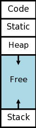
Areas (Segments) of Memory
As mentioned above, there are various OS issues we are ignoring,
for example the mapping from virtual to physical addresses, and
consequences of demand paging.
In this class we simply allocate memory segments in virtual memory
let the operating system worry about managing real memory.
In particular, we consider the following four areas of virtual memory.
- The code (often called text in OS-speak) is fixed size and
unchanging (self-modifying code is long out of fashion).
If there is OS support, the text could be marked execute only (or
perhaps read and execute, but not write).
All other areas would be marked non-executable.
- There is likely data of fixed size that can be determined by
the compiler by examining just the program's structure without
determining the program's execution pattern.
One example is global data.
Storage for this data would be allocated in the next area right
after the code.
A key point is that since the size of both the code and this
so-called
static
area do not change during execution,
these areas, unlike the next two so called dynamic
areas, have no need for an expansion region
.
- The stack is used for memory whose lifetime is stack-like.
It is organized into activation records that are created as a
procedure is called and destroyed when the procedure exits.
It abuts the area of unused memory so can grow easily.
Typically the stack is stored at the highest virtual addresses and
grows downward (toward small addresses).
However, it is sometimes easier in describing the activation
records and their uses to pretend that the addresses are
increasing (so that increments are positive).
We will discuss the stack in some detail below.
- The heap is used for data whose lifetime is not as easily
described.
This data is allocated by the program itself, typically either
with a language construct, such as
new
, or via a library
function call, such as malloc().
It is deallocated either by another executable statement, such as
a call to free(), or automatically by the system via
garbage collection
.
We will have little more to say about the heap.
7.1.1: Static Versus Dynamic Storage Allocation
Much (often most) data cannot be statically allocated.
Either its size is not known at compile time or its lifetime is
only a subset of the program's execution.
Early versions of Fortran used only statically allocated data.
This required that each array had a constant size specified in the
program.
Another consequence of supporting only static allocation was that
recursion was forbidden (otherwise the compiler could not tell how
many versions of a variable would be needed).
Modern languages, including newer versions of Fortran, support both
static and dynamic allocation of memory.
The advantage of supporting dynamic storage allocation is the
increased flexibility and storage efficiency possible (instead of
declaring an array to have a size adequate for the largest data set;
just allocate what is needed).
The advantage of static storage allocation is that it avoids the
runtime costs for allocation/deallocation and may permit faster code
sequences for referencing the data.
An (unfortunately, all too common) error is a so-called memory leak
where a long running program repeated allocates memory that it fails
to delete, even after it can no longer be referenced.
To avoid memory leaks and ease programming, several programming
language systems employ automatic garbage collection
.
That means the runtime system itself determines when data
can no longer be referenced and automatically deallocates it.
7.2: Stack Allocation of Space
The scheme to be presented achieves the following objectives.
- Memory is shared by procedure calls that have disjoint
durations.
Note that we are not able to determine disjointness by just
examining the program itself (due to data dependent branches
among other issues).
- The relative address of each (visible) nonlocal
variable is constant throughout each execution of a procedure.
Note that during this execution the procedure can call other
procedures.
7.2.1: Activation Trees
Recall the fibonacci sequence 1,1,2,3,5,8, ... defined by
f(1)=f(2)=1 and, for n>2, f(n)=f(n-1)+f(n-2).
Consider the function calls that result from a main program calling
f(5).
Surrounding the more-general pseudocode that calculates (very
inefficiently) the first 10 fibonacci numbers, we show the calls and
returns that result from main calling f(5).
On the left they are shown in a linear fashion and, on the right, we
show them in tree form.
The latter is sometimes called the activation tree or call tree.
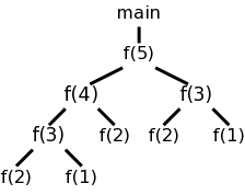
  System starts main                  int a[10];
      enter f(5)                      int main(){
          enter f(4)                      int i;
              enter f(3)                  for (i=0; i<10; i++){
                  enter f(2)                a[i] = f(i);
                  exit f(2)               }
                  enter f(1)          }
                  exit f(1)           int f (int n) {
              exit f(3)                   if (n<3)  return 1;
              enter f(2)                  return f(n-1)+f(n-2);
              exit f(2)               }
          exit f(4)
          enter f(3)
              enter f(2)
              exit f(2)
              enter f(1)
              exit f(1)
          exit f(3)
      exit f(5)
  main ends
We can make the following observations about these procedure
calls.
- If an activation of p calls q, then that activation of p
terminates no earlier than the activation of q.
- The order of activations (procedure calls) corresponds to a
preorder traversal of the call tree.
- The order of de-activations (procedure returns) corresponds to
postorder traversal of the call tree.
- The Euler-tour order captures both calls and returns.
- While executing a node N of the activation tree, the currently
live activations are those corresponding to N and its ancestors
in the tree.
- These live activations were called in the order given by the
root-to-N path in the tree, and the returns will occur in the
reverse order.
Homework: 1, 2.
7.2.2: Activation Records (ARs)
The information needed for each invocation of a procedure is kept
in a runtime data structure called an activation record
(AR) or frame.
The frames are kept in a stack called the control stack.
Note that this is memory used by the compiled program, not by the
compiler.
The compiler's job is to generate code that first obtains the needed
memory and second references the data stored in the ARs.
At any point in time the number of frames on the stack is the
current depth of procedure calls.
For example, in the fibonacci execution shown above when f(4) is
active there are three activation records on the control stack.
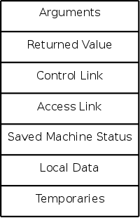
ARs vary with the language and compiler implementation.
Typical components are described below and pictured to the right.
In the diagrams the stack grows down the page.
- The arguments (sometimes called the
actual
parameters
).
The first few arguments are often instead placed in registers.
- The returned value.
This also is often instead placed in a register (if it is a
scalar).
- The control link.
These pointers connect the ARs by pointing from the AR of the
called routing to the AR of the caller.
- The access link.
This link is used to reference non-local variables in languages
with nested procedures, an interesting challenge that we discuss
in some detail below.
- Saved status from the caller, which typically includes the
return address and the machine registers.
The register values are restored when control returns to the
caller.
- Data local to the procedure being activated.
- Temporaries.
For example, recall the temporaries generated during expression
evaluation.
Often these can be held in machine registers.
When that is not possible, e.g., when there are more temporaries
than registers the temporary area is used.
Actually we will see in chapter 8 that only
live
temporaries are relevant.
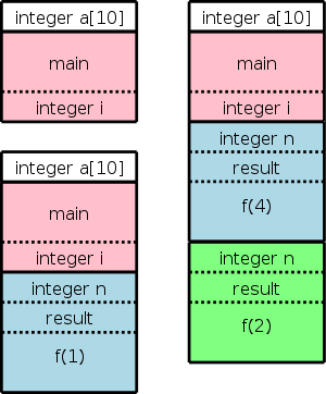
The diagram on the right shows (part of) the control stack for the
fibonacci example at three points during the execution.
The solid lines separate ARs; the dashed lines separate components
within an AR.
In the upper left we have the initial state.
We show the global variable a although it is not in an activation
record.
It is instead statically allocated before the program begins
execution (recall that the stack and heap are each dynamically
allocated).
Also shown is the activation record for main, which contains storage
for the local variable i.
Recall that local variables are near the end of the AR.
Below the initial state we see the next state when main has called
f(1) and there are two activation records, one for main and one for
f.
The activation record for f contains space for the argument n and
and also for the returned value.
Recall that arguments and the return value are allocated near the
beginning of the AR.
There are no local variables in f.
At the far right is a later state in the execution when f(4) has
been called by main and has in turn called f(2).
There are three activation records, one for main and two for f.
It is these multiple activations for f that permits the recursive
execution.
There are two locations for n and two for the returned value.
7.2.3: Calling Sequences
The calling sequence, executed when one procedure (the
caller) calls another (the callee), allocates an activation record
(AR) on the stack and fills in the fields.
Part of this work is done by the caller; the remainder by the
callee.
Although the work is shared, the AR is referred to as the callee's
AR.
Since the procedure being called is defined in one place, but
normally called from many places, we would expect to find more
instances of the caller activation code than of the callee
activation code.
Thus it is wise, all else being equal, to assign as much of the work
to the callee as possible.
Although details vary among implementations, the following
principle is often followed: Values computed by the caller are
placed before any items of size unknown by the caller.
This way they can be referenced by the caller using fixed offsets.
One possible arrangement is the following.
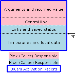
-
Place values computed by the caller at the beginning of the
activation record, i.e., adjacent to AR of the caller.
- The number of arguments may not be the same for different calls
of the same function (so called varargs, e.g. printf() in C).
However the (compiler of the) caller knows how many arguments
there are at this call site so, where pink calls blue, the
compilers knows how far the return value is from the beginning
of the blue AR.
- Since this beginning of the blue AR is the end of the pink AR
(or is one location further depending on how you count), the
caller knows (but only at run time) the offset of the return
value location from its own stack pointer (sp, see
below).
- Fixed length items are placed next.
Their sizes are known to the caller and callee at compile time.
Examples of fixed length items include the links and the saved
status.
- Finally come items allocated by the callee whose size is known
only at run-time, e.g., arrays whose size depends on the
parameters.
- The stack pointer sp is conveniently placed as shown in
diagram.
Note three consequences of this choice.
- The temporaries and local data are actually above
the stack.
This would seem even more surprising if I used the book's
terminology, which is top_sp.
- Fixed length data can be referenced by fixed offsets
(known to the intermediate code generator) from the sp.
- The caller knows the distance from the beginning of the
callee's AR to the sp and hence can set the sp when making
the call.
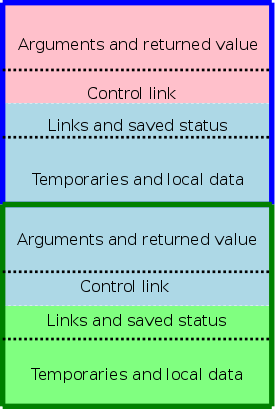
The picture above illustrates the situation where a pink procedure
(the caller) calls a blue procedure (the callee).
Also shown is Blue's AR.
It is referred to as Blue's AR because its lifetime matches
that of Blue even though responsibility for this single AR is shared
by both procedures.
The picture is just an approximation: For example, the returned
value is actually Blue's responsibility, although the space might
well be allocated by Pink.
Naturally, the returned value is only relevant for functions, not
procedures.
Also some of the saved status, e.g., the old sp, is saved by Pink.
The picture to the right shows what happens when Blue, the callee,
itself calls a green procedure and thus Blue is also a caller.
You can see that Blue's responsibility includes part of its AR as
well as part of Green's.
Actions During the Call
The following actions occur during a call.
- The caller begins the process of creating the callee's AR by
evaluating the arguments and placing them in the AR of the
callee.
(I use arguments for the caller, parameters for the
callee.)
- The caller stores the return address and the
(soon-to-be-updated) sp in the callee's AR.
- The caller increments sp so that instead of pointing into its
AR, it points to the corresponding point in the callee's
AR.
- The callee saves the registers and other (system dependent)
information.
- The callee allocates and initializes its local data.
- The callee begins execution.
Actions During the Return
When the procedure returns, the following actions are performed by
the callee, essentially undoing the effects of the calling sequence.
- The callee stores the return value (if the callee is a
function).
- The callee restores sp and the registers.
- The callee jumps to the return address.
Note that varargs are supported.
Also note that the values written during the calling sequence are
not erased and the space is not explicitly reclaimed.
Instead, the sp is restored and, if and when the caller makes
another call, the space will be reused.
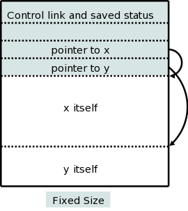
7.2.4: Variable-Length Data on the Stack
There are two flavors of variable-length data.
- Data obtained by malloc/new have hard to determine lifetimes
and are stored in the heap instead of the stack.
- Data, such as arrays with bounds determined by the parameters
are still stack like in their lifetimes (if A calls B, these
variables of A are allocated before and released after the
corresponding variables of B).
It is the second flavor that we wish to allocate on the stack.
The goal is for the callee to be able to access these arrays using
addresses determined at compile time even though the size of the
arrays is not known until the program is called, and indeed often
differs from one call to the next (even when the two calls
correspond to the same source statement).
The solution is to leave room for pointers to the arrays in the AR.
These pointers are fixed size and can thus be accessed using offsets
known at compile time.
When the procedure is invoked and the sizes are known, the pointers
are filled in and the space allocated.
A difficulty caused by storing these variable size items on the
stack is that it no longer is obvious where the real top of the
stack is located relative to sp.
Consequently another pointer (we might call it real-top-of-stack) is
also kept.
This pointer tells the callee where to begin a new AR if the callee
itself makes a call.
An alternate, probably more common name for the
(stack-pointer, real-top-of-stack-pointer) pair is
(stack-pointer, frame-pointer)
Homework: 4.
7.3: Access to Nonlocal Data on the Stack
As we shall see, the ability of procedure P to access data declared
outside of P (either declared globally outside of all procedures or,
especially, those declared inside another procedure Q with P nested
inside Q) offers interesting challenges.
7.3.1: Data Access Without Nested Procedures
In languages like standard C without nested procedures, visible
names are either local to the procedure in question or are declared
globally.
- For global names the address is known statically at compile time,
providing there is only one source file.
If there are multiple source files, the linker knows.
In either case no reference to the activation record is needed;
the addresses are known prior to execution.
- For names local to the current procedure, the address needed is
in the AR at a known-at-compile-time constant offset from the sp.
In the case of variable size arrays, the constant offset refers to
a pointer to the actual storage.
7.3.2: Issues With Nested Procedures
With nested procedures a complication arises.
Say g is nested inside f.
So g can refer to names declared in f.
These names refer to objects in the AR for f.
The difficulty is finding that AR when g is executing.
We can't tell at compile time where the (most
recent) AR for f will be relative to the current AR for g
since a dynamically-determined (i.e., unknown at compile time)
number of routines could have been called in the middle.
There is an example in the next section.
in which g refers to x, which is declared in the
immediately outer scope (main) but the AR is 2 away because f was
invoked in between.
(In that example you can tell at compile time what was called in
what order, but with a more complicated program having
data-dependent branches, it is not possible.)
7.3.3: A language with Nested Procedure Declarations
The book asserts (correctly) that C doesn't have nested procedures
so introduces ML, which does (and is quite slick).
However, many of you don't know ML and I haven't used it.
Fortunately, a common extension to C is to permit nested procedures.
In particular, gcc supports nested procedures.
To check my memory I compiled and ran the following program.
  #include <stdio.h>

  int main (int argc, char *argv[]) {
      int x = 10;

      int g(int y) {
	  int z = x+y;
	  return z;
      }

      int f (int y) {
	  return g(2*y);
      }

      (void) printf("The answer is %d\n", f(x));
      return 0;
  }
The program compiles without errors and the correct answer of 30 is
printed.
So we can use C (really the GCC extension of C) as the language to
illustrate nested procedure declarations.
Remark: Many consider this gcc extension (or its
implementation) to be evil.
For example, look
here,
here,
or
here.
7.3.4: Nesting Depth
Outermost procedures have nesting depth 1.
Other procedures have nesting depth 1 more than the nesting depth of
the immediately outer procedure.
In the example above, main has nesting depth 1; both f and g have
nesting depth 2.
7.3.5: Access Links
The AR for a nested procedure contains an access link that
points to the AR of the most recent activation of the immediately
outer procedure.
So in the example above the access link for f and the access link
for g would each point to the AR of the activation of main.
Then when g references x, defined in main, the activation record for
main can be found by following the access link in the AR for f.
Since f is nested in main, they are compiled together so, once the
AR is determined, the same techniques can be used as for variables
local to f.
This example was too easy.
- Everything can be determined at compile time since there are
no data dependent branches.
- This is only one AR for main during all of execution
since main is not (directly or indirectly) recursive and there
is only one AR for each of f and g.
However the technique is quite general.
For a procedure P to access a name defined in the 3-outer scope,
i.e., the unique outer scope whose nesting depth is 3 less than that
of P, you follow the access links three times.
Make sure you understand why the n-th outer scope,
but not the n-th inner scope is unique)
The remaining question is
How are access links maintained?
.
7.3.6: Manipulating Access Links
Let's assume there are no procedure parameters.
We are also assuming that the entire program is compiled at once.
For multiple files the main issues involve the linker, which is not
covered in this course.
I do cover it a little in the OS course.
Without procedure parameters, the compiler knows the name of the
called procedure and hence its nesting depth.
The compiler always knows the nesting depth of the caller.
Let the caller be procedure F and let the called procedure be G, so
we have F calling G.
Let N(proc) be the nesting depth of the procedure proc.
We distinguish two cases.
- N(G)>N(F).
The only way G can be visible in F and have a greater nesting
depth is for G to be declared immediately inside F.
Then when compiling the call from F to G it we simply set
the access link of G to point to the AR of F.
In this case the access link is the same as the control
link.
- N(G)≤N(F).
This includes the case F=G, i.e., a direct recursive call.
For G to be visible in F, there must be another procedure P
enclosing both F and G, with G immediately inside P.
That is, we have the following situation, where
k=N(G)-N(F)≥0
	P() {
          G() {...}
          P1() {
            P2() {
              ...
              Pk() {
                F(){... G(); ...}
              }
             ...
            }
          }
        }
Our goal while creating the AR for G at the call from F is to
set the access link to point to the AR for P.
Note that the entire structure in the skeleton code shown is
visible to the compiler.
The current (at the time of the call) AR is the one for F and,
if we follow the access links k times we get a pointer to the AR
for P, which we can then place in the access link for the
being-created AR for G.
The above works fine when F is nested (possibly deeply) inside G.
It is the picture above but P1 is G.
When k=0 we get the gcc code I showed before and also the case of
direct recursion where G=F.
I do not know why the book separates out the case k=0, especially
since the previous edition didn't.
7.3.7: Access Links for Procedure Parameters
The problem is that, if f calls g with a parameter of h (or a
pointer to h in C-speak) and then g calls this parameter (i.e.,
calls h), g might not know the context of h.
The solution is for f to pass to g the pair (h, the access link of
h) instead of just passing h.
Naturally, this is done by the compiler, the programmer is unaware
of access links.
7.3.8: Displays
The basic idea is to replace the linked list of access links, with
an array of direct pointers.
In theory access links can form long chains (in practice, nesting
depth rarely exceeds a dozen or so).
A display is an array in which entry i points to the most recent
(highest on the stack) AR of depth i.
7.4: Heap Management
Almost all of this section is covered in the OS class.
7.4.1: The Memory Manager
Covered in OS.
7.4.2: The Memory Hierarchy of a Computer
Covered in Architecture.
7.4.3: Locality in Programs
Covered in OS.
7.4.4: Reducing (external) Fragmentation
Covered in OS.
7.4.5: Manual Deallocation Requests
Stack data is automatically deallocated when the defining procedure
returns.
What should we do with heap data explicated allocated with
new/malloc?
The manual method is to require that the programmer explicitly
deallocate these data.
Two problems arise.
- Memory leaks.
The programmer forgets to deallocate.
        loop
            allocate X
            use X
            forget to deallocate X
	end loop
As this program continues to run it will require more and more
storage even though is actual usage is not increasing
significantly.
- Dangling References.
The programmer forgets that they did a deallocate.
        allocate X
        use X
        deallocate X
        100,000 lines of code not using X
        use X
Both can be disastrous and motivate the next topic, which is
covered in programming languages courses.
7.5: Introduction to Garbage Collection
The system detects data that cannot be accessed (no direct or
indirect references exist) and deallocates the data automatically.
Covered in programming languages.
7.5.1: Design Goals for Garbage Collectors
7.5.2: Reachability
7.5.3: Reference Counting Garbage Collectors
7.6: Introduction to Trace-Based Collection
7.6.1: A Basic Mark-and-Sweep Collector
7.6.2:Basic Abstraction
7.6.3: Optimizing Mark-and-Sweep
7.6.4: Mark-and-Compact Garbage Collectors
7.6.5: Copying Collectors
7.6.6: Comparing Costs
7.7: Short Pause Garbage Collection
7.7.1: Incremental Garbage Collection
7.7.2: Incremental Reachability Analysis
7.7.3: Partial Collection Basics
7.7.4: Generational Garbage Collection
7.7.5: The Train Algorithm
7.8: Advanced Topics in Garbage Collection
7.8.1: Parallel and Concurrent Garbage Collection
7.8.2: Partial Object Relocation
7.8.3: Conservative Collection for Unsafe Languages
7.8.4: Weak References
Start Lecture #13
Chapter 8: Code Generation
Homework: Read Chapter 8.
Goal: Transform the intermediate code and tables produced by the
front end into final machine (or assembly) code.
Code generation plus optimization constitutes the back end of the
compiler.
8.1: Issues in the Design of a Code Generator
8.1.1: Input to the Code Generator
As expected the input to the code generator is the output of the
intermediate code generator.
We assume that all syntactic and semantic error checks have been
done by the front end.
Also, all needed type conversions are already done and any type
errors have been detected.
We are using three address instructions for our intermediate
language.
These instructions have several representations, quads, triples,
indirect triples, etc.
In this chapter I will tend to use the term quad (for brevity) when
I should really say three-address instruction, since the
representation doesn't matter.
8.1.2: the Target Program
A RISC (Reduced Instruction Set Computer), e.g. PowerPC, Sparc,
MIPS (popular for embedded systems), is characterized by
- Many registers.
- Three address instructions.
- Simple addressing modes.
- Relatively simple ISA (instruction set architecture).
Only
loads and stores touch memory.
- Homogeneous registers.
- Very few instruction lengths.
A CISC (Complex Instruct Set Computer), e.g. x86, x86-64/amd64 is
characterized by
- Few registers.
- Two address instructions.
- Variety of addressing modes (some complex).
- Complex ISA.
- Register classes.
- Multiple instruction lengths.
A stack-based computer is characterized by
No
registers.
- Zero address instructions (operands and results are implicitly
on the runtime stack).
- The top portion of the stack is kept in hidden registers.
An accumulator-based computer is characterized by
- One special register (the accumulator) where results are
placed.
- Other (index) registers often used in loops for the index and
to help specify the address of an array element.
- One address instructions (the other operand is the accumulator).
A Little History
IBM 701/704/709/7090/7094 (Moon shot, MIT CTSS) were accumulator based.
Stack based machines were believed to be good compiler targets.
They became very unpopular when it was believed that register
architecture would perform better.
Better compilation (code generation) techniques appeared that could
take advantage of the multiple registers.
Pascal P-code and Java byte-code are the machine instructions for a
hypothetical stack-based machines, the JVM (Java Virtual Machine) in
the case of Java.
This code can be interpreted or compiled to native code.
RISC became all the rage in the 1980s.
CISC made a gigantic comeback in the 90s with the intel pentium
pro.
A key idea of the pentium pro is that the hardware would
dynamically translate a complex x86 instruction into a series of
simpler RISC-like
instructions called ROPs (RISC ops).
The actual execution engine dealt with ROPs.
The jargon would be that, while the architecture (the ISA) remained
the x86, the micro-architecture was quite different and more like
the micro-architecture seen in previous RISC processors.
Assemblers and Linkers
For maximum compilation speed of modest size programs, the compiler
accepts the entire program at once and produces code that can be
loaded and executed (the compilation system can include a simple
loader and can start the compiled program).
This was popular for student jobs
when computer time was
expensive.
The alternative, where each procedure can be compiled separately,
requires a linkage editor.
It eases the compiler's task to produce assembly code instead of
machine code and we will do so.
This decision increases the total compilation time since it requires
an extra assembler pass (or two).
8.1.3: Instruction Selection
A big question is the level of code quality we seek to attain.
For example we can simply translate one quadruple at a time.
The quad
x = y + z
can always (assuming the addresses x, y, and z are each a compile
time constant off a given register, e.g., the sp) be compiled
into 4 RISC-like instructions (fewer CISC instructions would
suffice) using only 2 registers R0 and R1.
    LD  R0, y
    LD  R1, z
    ADD R0, R0, R1
    ST  x, R0
But if we apply this to each quad separately (i.e., as a separate
problem) then
    a = b + c
    d = a + e
is compiled into
    LD  R0, b
    LD  R1, c
    ADD R0, R0, R1
    ST  a, R0
    LD  R0, a
    LD  R1, e
    ADD R0, R0, R1
    ST  d, R0
The fifth statement is clearly not needed since we are loading into
R0 the same value that it contains.
This inefficiency is caused by our compiling the second quad with no
knowledge of how we compiled the first quad.
8.1.4: Register Allocation
Since registers are the fastest memory in the computer, the ideal
solution is to store all values in registers.
However, there are normally not nearly enough registers for this to
be possible.
So we must choose which values are in the registers at any given time.
Actually this problem has two parts.
- Which values should be stored in registers?
- Which register should each selected value be stored in
The reason for the second problem is that often there are register
requirements, e.g., floating-point values in floating-point
registers and certain requirements for even-odd register pairs
(e.g., 0&1 but not 1&2) for multiplication/division.
We shall concentrate on the first problem.
8.1.5: Evaluation Order
Sometimes better code results if the quads are reordered.
One example occurs with modern processors that can execute multiple
instructions concurrently, providing certain restrictions are met
(the obvious one is that the input operands must already be
evaluated).
8.2: The Target Language
This is a delicate compromise between RISC and CISC.
The goal is to be simple but to permit the study of nontrivial
addressing modes and the corresponding optimizations.
A charging
scheme is instituted to reflect that complex addressing
modes are not free.
8.2.1: A Simple Target Machine Model
We postulate the following (RISC-like) instruction set
-
Load. LD dest, addr
loads the destination dest with the contents of the
address addr.
LD reg1, reg2
is a register copy.
A question is whether dest can be a memory location
or whether it must be a register.
This is part of the RISC/CISC debate.
In CISC parlance, no distinction is made between load and
store, both are examples of the general move instruction that
can have an arbitrary source and an arbitrary destination.
We will normally not use a memory location for the
destination of a load (or the source of a store).
This implies that we are not able to perform a memory to memory
copy in one instruction.
As will be seen below, in those places where a memory
location is permitted, we charge more than for a register.
-
Store. ST addr, src
stores the value of the source src (register) into
the address addr.
We do permit an integer constant preceded by a number sign,
(e.g., #181
) to be used instead of a register, but again
we charge extra.
-
Computation. OP dest, src1, src2
or dest = src1 OP
src2
performs the operation OP on the two source operands
src1 and src2.
For a RISC architecture the three operands must be registers.
This will be our emphasis (extra charge for an
integer src).
If the destination register is one of the sources, the source
is read first and then overwritten (in one cycle by utilizing
a master-slave flip-flop, when both are registers.)
-
Unconditional branch. BR L
transfers control to the (instruction with) label L.
When used with an address rather than a label it means to
goto that address.
Note that we are using the l-value of the address.
Remark: This is unlike the situation with a
load instruction in which case the r-value i.e.,
the contents of the address, is loaded into
the register.
Please do not be confused by this usage.
The address or memory address always refers to the location,
i.e., the l-value.
Some instructions, e.g., LD, require that the
location be dereferenced, i.e, that the r-value be
obtained
-
Conditional Branch. Bcond r, L
transfers to the label (or location) L if register
r satisfies the condition cond.
For example,
BNEG R0, joe
branches to joe if
R0 is negative.
Addressing modes
The addressing modes are not simply RISC-like, as they permit
indirection through memory locations.
Again, note that we shall charge extra for some such operands.
Recall the difference between an l-value and an r-value, e.g. the
difference between the uses of x in
x = y + 3
and
z = x + 12
The first refers to an address, the second to a value
(stored in that address).
We assume the machine supports the following addressing modes.
-
Variable name.
This is shorthand (or assembler-speak) for the memory location
containing the variable, i.e., we use the l-value of the
variable name.
So
LD R1, a
sets the contents of R1 equal to the contents of
a, i.e.,
contents(R1) := contents(a)
Do not get confused here.
The l-value of a is used as the address (that is what the
addressing mode tells us).
But the load instruction itself loads the first operand with
the contents of the second.
That is why it is the r-value of the second operand that is
placed into the first operand.
-
Indexed address.
The address a(reg), where a is a variable name and
reg is a register (i.e., a register number), specifies the
address that is the r-value-of-reg bytes past the address
specified by a.
That is, the address is computed as the l-value of a plus the
r-value of reg.
So
LD r1, a(r2)
sets
contents(r1) :=
contents(a+contents(r2))
NOT
contents(r1) :=
contents(contents(a)+contents(r2))
Permitting this addressing mode outside a load or store
instruction, which we shall not do, would strongly suggest a
CISC architecture.
-
Indexed constant.
An integer constant can be indexed by a register.
So
LD r1, 8(r4)
sets
contents(r1) :=
contents(8+contents(r4)).
In particular,
LD r1, 0(r4)
sets
contents(r1) :=
contents(contents(r4)).
-
Indirect addressing.
If I is an integer constant and r is a
register, the previous addressing mode tells us that
I(r) refers to the address
I+contents(r).
The new addressing mode *I(r) refers to the address
contents(I+contents(r)).
The address *r is shorthand for *0(r).
The address *10 is shorthand for
*10(fakeRegisterContainingZero).
So
LD r1, *50(r2)
sets
contents(r1) :=
contents(contents(50+contents(r2))).
and
LD r1, *r2
sets
(get ready)
contents(r1) :=
contents(contents(contents(r2)))
and
LD r1, *10
sets
contents(r1) :=
contents(contents(10))
-
Immediate constant.
If a constant is preceded by a # it is treated as an r-value
instead of as a register number.
So
ADD r2, r2, #1
is an increment instruction.
Indeed
ADD 2, 2, #1
does the same thing, but we probably won't write that; for
clarity we will normally write registers beginning with an
r
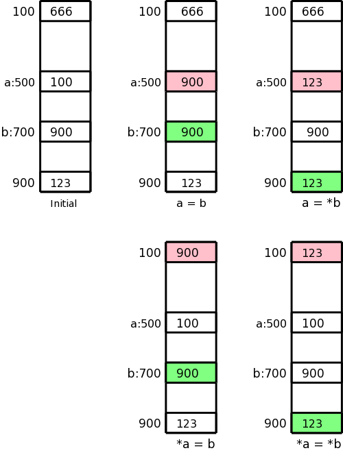
Addressing Mode Usage
Remember that in 3-address instructions, the variables written are
addresses, i.e., they represent l-values.
Let us assume the l-value of a is 500 and the l-value b is 700,
i.e., a and b refer to locations 500 and 700 respectively.
Assume further that location 100 contains 666, location 500 contains
100, location 700 contains 900, and location 900 contains 123.
This initial state is shown in the upper left picture.
In the four other pictures the contents of the pink location has
been changed to the contents of the light green location.
These correspond to the three-address assignment statements shown
below each picture.
The machine instructions indicated below implement each of these
assignment statements.
    a = b
    LD  R1, b
    ST  a, R1

    a = *b
    LD  R1, b
    LD  R1, 0(R1)
    ST  a, R1

    *a = b
    LD  R1, b
    LD  R2, a
    ST  0(R2), R1

    *a = *b
    LD  R1, b
    LD  R1, 0(R1)
    LD  R2, a
    ST  0(R2), R1
Naive Translation of Quads to Instructions
For many quads the naive (RISC-like) translation is 4 instructions.
- Load the first source into a register.
- Load the second source into another register.
- Do the operation.
- Store the result.
Array assignment statements are also four instructions.
We can't have a quad A[i]=B[j] because that needs four addresses and
quads have only three.
Similarly, we can't use an array in a computation statement like
a[i]=x+y because it again would need four addresses.
The instruction x=A[i] becomes (assuming each element of A is 4
bytes.
Actually, our intermediate code generator already does the
multiplication so we would not generate a multiply here).
    LD  R0, i
    MUL R0, R0, #4
    LD  R0, A(R0)
    ST  x, R0
Similarly A[i]=x becomes (again our intermediate code generator
already does the multiplication).
    LD  R0, i
    MUL R0, R0, #4
    LD  R1, x
    ST  A(R0), R1
The (C-like) pointer reference x = *p becomes
    LD  R0, p
    LD  R0, 0(R0)
    ST  x, R0
The assignment through a pointer *p = x becomes
    LD  R0, x
    LD  R1, p
    ST  0(R1), R0
Finally, if x < y goto L becomes
    LD   R0, x
    LD   R1, y
    SUB  R0, R0, R1
    BNEG R0, L
Conclusion
With a modest amount of additional effort much of the output of lab
4 could be turned into naive assembly language.
We will not do this.
Instead, we will spend the little time remaining learning how to
generate less-naive assembly language.
8.2.2: Program and Instruction Costs
Generating good code requires that we have a metric, i.e., a way of
quantifying the cost of executing the code.
The run-time cost of a program depends on (among other factors)
- The cost of the generated instructions.
- The number of times the instructions are executed.
Here we just determine the first cost, and use quite a simple metric.
We charge for each instruction one plus the cost of each addressing
mode used.
Addressing modes using just registers have zero cost, while those
involving memory addresses or constants are charged one.
None of our addressing modes have both a memory address and a
constant or two of either one.
The charge corresponds to the size of the instruction since a memory
address or a constant is assumed to be stored in a word right after
the instruction word itself.
You might think that we are measuring the memory (or space) cost of
the program not the time cost, but this is mistaken:
The primary space cost is the size of the data, not the size of the
instructions.
One might say we are charging for the pressure on the I-cache.
For example, LD R0, *50(R2) costs 2, the additional cost is for the
constant 50.
I believe that the book special cases the addresses 0(reg) and
*0(reg) so that the 0 is not explicitly stored and not charged for.
The significance for us is calculating the length an instruction such
as
LD R1, 0(R2)
We care about the length of an instruction when we need to generate
a branch that skips over it.
Homework: 1, 2, 3, 4.
Calculate the cost for 2c.
8.3: Address in the Target Code
There are 4 possibilities for addresses that must be generated
depending on which of the following areas the address refers to.
- The text or code area.
The location of items in this area is statically determined,
i.e., is known at compile time.
- The static area holding global constants.
The location of items in this area is statically determined.
- The stack holding activation records.
The location of items in this area is not known at compile time.
- The heap.
The location of items in this area is not known at compile time.
8.3.1: Static Allocation
Returning to the glory days of Fortran, we first consider a system
with only static allocation, i.e., with all address in the first two
classes above.
Remember, that with static allocation we know before execution where
all the data will be stored.
There are no recursive procedures; indeed, there is no run-time
stack of activation records.
Instead the ARs (one per procedure) are statically
allocated by the compiler.
Caller Calling Callee
In this simplified situation, calling a parameterless procedure just
uses static addresses and can be implemented by two instructions.
Specifically,
call callee
can be implemented by
    ST  callee.staticArea, #here+20
    BR  callee.codeArea
Assume, for convenience, that the return address is the
first location in the activation record (in general, for a
parameterless procedure, the return address would be a
fixed offset from the beginning of the AR).
We use the attribute staticArea for the address of the AR for the
given procedure (remember again that there is no stack and no heap).
What is the mysterious #here+20?
We know that # signifies an immediate constant.
We use here to represent the address of the current
instruction (the compiler knows this value since we are assuming
that the entire program, i.e., all procedures, are compiled at
once).
The two instructions listed contain 3 constants, which means that
the entire sequence takes 2+3=5 words or 20 bytes.
Thus here+20 is the address of the instruction after the BR, which
is indeed the return address.
Callee Returning
With static allocation, the compiler knows the address of the
the AR for the callee and we are assuming that the return address is
the first entry.
Then a procedure return is simply
BR *callee.staticArea
Let's make sure we understand the indirect addressing here.
The value callee.staticArea is the address of a memory location
into which the caller placed the return address.
So the branch is not to callee.staticArea, but instead to the
return address, which is the value contained in
callee.staticArea.
Note: You might well wonder why the load
LD r0, callee.staticArea
places the contents of callee.staticArea into R0
without needing a *.
The answer, as mentioned above, is that branch and load have
different semantics: Both take an address as an argument, branch
jumps to that address, whereas, load retrieves the
contents.
Example
We consider a main program calling a procedure P and then
halting.
Other actions by Main and P are indicated by subscripted uses
of other
.
  // Quadruples of Main
  other1
  call P
  other2
  halt
  // Quadruples of P
  other3
  return
Let us arbitrarily assume that the code for Main starts in location
1000 and the code for P starts in location 2000 (there might be
other procedures in between).
Also assume that each otheri requires 100 bytes (all
addresses are in bytes).
Finally, we assume that the ARs for Main and P begin at 3000 and
4000 respectively.
Then the following machine code results.
// Code for Main
1000: Other1
1100: ST 4000, #1120 // P.staticArea, #here+20
1112: BR 2000 // Two constants in previous instruction take 8 bytes
1120: other2
1220: HALT
...
// Code for P
2000: other3
2100: BR *4000
...
// AR for Main
3000: // Return address stored here (not used
)
3004: // Local data for Main starts here
...
// AR for P
4000: // Return address stored here
4004: // Local data for P starts here
8.3.2: Stack Allocation
We now need to access the ARs from the stack.
The key distinction is that the location of the current AR
is not known at compile time.
Instead a pointer to the stack must be maintained dynamically.
We dedicate a register, call it SP, for this purpose.
In this chapter we let SP point to the bottom of the current AR,
that is the entire AR is above the SP.
Since we are not supporting varargs, there is no advantage to having
SP point to the middle
of the AR as in the previous chapter.
The main procedure (or the run-time library code called before
any user-written procedure) must initialize SP with
LD SP, #stackStart
where stackStart is a known-at-compile-time constant.
The caller increments SP (which now points to the beginning of its
AR) to point to the beginning of the callee's AR.
This requires an increment by the size of
the caller's AR, which of course the caller knows.
Is this size a compile-time constant?
The book treats it as a constant.
The only part that is not known at compile time is the size of the
dynamic arrays.
Strictly speaking this is not part of the AR, but it must be skipped
over since the callee's AR starts after the caller's dynamic arrays.
Perhaps for simplicity we are assuming that there are no dynamic
arrays being stored on the stack.
If there are arrays, their size must be included in some way.
Caller Calling Callee
The code generated for a parameterless call is
    ADD SP, SP, #caller.ARSize
    ST  0(SP), #here+16        // save return address (book wrong)
    BR  callee.codeArea
Callee Returning
The return requires code from both the Caller and Callee.
The callee transfers control back to the caller with
BR *0(SP)
Upon return the caller restore the stack pointer with
SUB SP, SP, #caller.ARSize
Example
We again consider a main program calling a procedure P and then
halting.
Other actions by Main and P are indicated by subscripted uses of
`other'.
    // Quadruples of Main
    other1
    call P
    other2
    halt
    // Quadruples of P
    other3
    return
Recall our assumptions that the code for Main starts in location
1000, the code for P starts in location 2000, and each
otheri requires 100 bytes.
Let us assume the stack begins at 9000 (and grows to larger
addresses) and that the AR for Main is of size 400 (we don't need
P.ARSize since P doesn't call any procedures).
Then the following machine code results.
    // Code for Main
    1000: LD  SP, 9000        // Possibly done prior to Main
    1008: Other1
    1108: ADD SP, SP, #400
    1116: ST  0(SP), #1132    // Understand the address
    1124: BR, 2000
    1132: SUB SP, SP, #400
    1140: other2
    1240: HALT
    ...
    // Code for P
    2000: other3
    2100: BR *0(SP)           // Understand the *
    ...
    // AR for Main
    9000:                     // Return address stored here (not used)
    9004:                     // Local data for Main starts here
    9396:                     // Last word of the AR is bytes 9396-9399
    ...
    // AR for P
    9400:                     // Return address stored here
    9404:                     // Local data for P starts here
    9496:                     // Last word of the AR is bytes 9496-9799
Homework: 1, 2, 3.
8.3.3: Run-Time Addresses for Names
A technical fine point about static allocation and a
corresponding point about the display.
8.4: Basic Blocks and Flow Graphs
As we have seen, for many quads it is quite easy to generate a
series of machine instructions to achieve the same effect.
As we have also seen, the resulting code can be quite inefficient.
For one thing the last instruction generated for a quad is often a
store of a value that is then loaded right back in the next quad (or
one or two quads later).
Another problem is that we don't make much use of the registers.
That is, translating a single quad needs just one or two registers so
we might as well throw out all the other registers on the machine.
Both of the problems are due to the same cause:
Our horizon is too limited.
We must consider more than one quad at a time.
But wild flow of control can make it unclear which quads
are dynamically
near each other.
So we want to consider, at one time, a group of quads for which
the dynamic order of execution is tightly controlled.
We then also need to understand how execution proceeds from one
group to another.
Specifically the groups are called basic blocks and the
execution order among them is captured by the flow graph.
Definition:
A basic block is a maximal collection of consecutive quads
such that
- Control enters the block only at the first instruction.
- Branches (or halts) occur only at the last instruction.
Definition:
A flow graph has the basic blocks as vertices and has edges
from one block to each possible dynamic successor.
We process all the quads in a basic block together
making
use of the fact that the block is not entered or left in
the middle
.
8.4.1: Basic Blocks
Constructing the basic blocks is easy.
Once you find the start of a block, you keep going until you hit a
label or jump.
But, as usual, to say it correctly takes more words.
Definition:
A basic block leader (i.e., first instruction) is any of the
following (except for the instruction just past the entire program).
- The first instruction of the program.
- A target of a (conditional or unconditional) jump.
- The instruction immediately following a jump.
Given the leaders, a basic block starts with a leader and proceeds
up to but not including the next leader.
Example
The following code produces a 10x10 real identity matrix
    for i from 1 to 10 do
      for j from 1 to 10 do
        a[i,j] = 0
      end
    end
    for i from 1 to 10 do
      a[i,i] = 1.0
    end
The following quads do the same thing.
Don't worry too much about how the quads were generated.
     1)  i = 1
     2)  j = 1
     3)  t1 = 10 * i
     4)  t2 = t1 + j        // element [i,j]
     5)  t3 = 8 * t2        // offset for a[i,j] (8 byte reals)
     6)  t4 = t3 - 88       // program array starts at [1,1] assembler at [0,0]
     7)  a[t4] = 0.0
     8)  j = j + 1
     9)  if j <= 10 goto (3)
    10)  i = i + 1
    11)  if i <= 10 goto (2)
    12)  i = 1
    13)  t5 = i - 1
    14)  t6 = 88 * t5
    15)  a[t6] = 1.0
    16)  i = i + 1
    17)  if i <= 10 goto (13)
Which quads are leaders?
1 is a leader by definition.
The jumps are 9, 11, and 17.
So 10 and 12 are leaders as are the targets 3, 2, and 13.
The leaders are then 1, 2, 3, 10, 12, and 13.
The basic blocks are therefore {1}, {2}, {3,4,5,6,7,8,9}, {10,11},
{12}, and {13,14,15,16,17}.
Here is the code written again with the basic blocks indicated.
     1)  i = 1

     2)  j = 1

     3)  t1 = 10 * i
     4)  t2 = t1 + j            // element [i,j]
     5)  t3 = 8 * t2            // offset for a[i,j] (8 byte numbers)
     6)  t4 = t3 - 88           // we start at [1,1] not [0,0]
     7)  a[t4] = 0.0
     8)  j = j + 1
     9)  if J <= 10 goto (3)

    10)  i = i + 1
    11)  if i <= 10 goto (2)

    12)  i = 1

    13)  t5 = i - 1
    14)  t6 = 88 * t5
    15)  a[t6] = 1.0
    16)  i = i + 1
    17)  if i <= 10 goto (13)
We can see that once you execute the leader you are assured of
executing the rest of the block in order.
Start Lecture #14
8.4.2: Next Use Information
We want to record the flow of information from instructions that
compute a value to those that use the value.
One advantage we will achieve is that if we find a value has no
subsequent uses, then it is dead and the register holding that value
can be used for another value.
Assume that a quad p assigns a value to x (some would call this
a def of x).
Definition:
A quad q uses the value computed at p (uses
the def) and x is live at q
if q has x as an operand and there is a possible execution path from
p to q that does not pass any other def of x.
Since the flow of control is trivial inside a basic block, we are
able to compute the live/dead status and next use information at the
block leader by a simple backwards scan of the quads (algorithm
below).
Note that if x is dead (i.e., defined before used) on entrance to B
the register containing x can be reused in B.
Computing Live/Dead and Next Use Information
Our goal is to determine whether a block uses a value and if so in
which statement is it first used.
The following algorithm for computing uses is quite simple.
    Initialize all variables in B as being live
    Examine the quads q of the block in reverse order.
        Assume the quad q computes x and reads y and z
        Mark x as dead; mark y and z as live and used at q
When the loop finishes those values that are read before being
written are marked as live and their first use is noted.
The locations x that are written before being read are marked dead
meaning that the value of x on entrance is not used.
Those values that are neither read nor written remain simply live.
They are not dead since the dynamically next
basic block might use them.
Note that we have determined whether values are live/dead on
entrance to the basic block.
We would like to know as well if they are live/dead on exit, but
that requires global flow analysis, which we do not know.
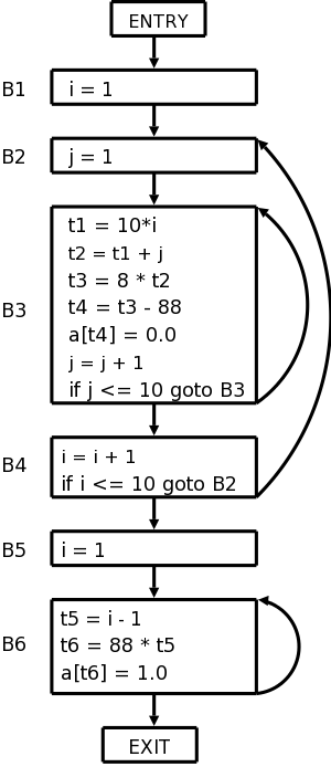
8.4.3: Flow Graphs
The nodes of the flow graph are the basic blocks, and there is an
edge from P (predecessor) to S (successor) if S might follow P.
More formally, such an edge is added if the last statement of P
- is a jump to S (it must be to the leader of S) or
- is NOT an UNCONDITIONAL jump
and S immediately follows P.
(Note that the figure on the right satisfies this condition for
every basic block.
Do NOT assume that is always the case.
Two nodes are added: entry
and exit
.
An edge is added from entry to the first basic block, i.e. the block
that has the first statement of the program as leader.
Edges to the exit are added from any block that could be the last
block executed.
Specifically, edges are added to exit from
- the last block if it doesn't end in an unconditional jump.
- any block that ends in a jump to outside the program.
The flow graph for our example is shown on the right.
8.4.4: Representing Flow Graphs
Note that jump targets are no longer quads but blocks.
The reason is that various optimizations within blocks will change
the instructions and we would have to change the jump to reflect
this.
8.4.5: Loops
For most programs the bulk of the execution time is within loops so
we want to identify these.
Definition:
A collection of basic blocks forms a
loop L
with
loop entry E if
- No block in L other than E has a predecessor outside L.
- All blocks in L have a path to E completely inside L.
The flow graph on the right has three loops.
- {B3}, i.e., B3 by itself.
- {B6}.
- {B2, B3, B4}
Homework: 1.
Remark:
Nothing beyond here will be on the final.
A Word or Two About Global Flow Analysis
We are not covering global flow analysis; it is a key component of
optimization and would be a natural topic in a follow-on course.
Nonetheless there is something we can say just by examining the flow
graphs we have constructed.
For this discussion I am ignoring tricky and important
issues concerning arrays and pointer references (specifically,
disambiguation).
You may wish to assume that the program contains no arrays or
pointers.
We have seen that a simple backwards scan of the statements in a
basic block enables us to determine the variables that are
live-on-entry (and their first use) and those variables that are
dead-on-entry.
Those variables that do not occur in the block are considered live
but with no next use; perhaps it would be better to call
them ignored by the block
.
We shall see below that it would be lovely to know which variables
are live/dead-on-exit.
This means which variables hold values at the end of the block that
will / will not be used.
To determine the status of v on exit of a block B, we need to trace
all possible execution paths beginning at the end of B.
If all these paths reach a block where v is dead-on-entry before
they reach a block where v is live-on-entry, then v is dead on exit
for block B.
8.5: Optimization of Basic Blocks
8.5.1: The DAG Representation of Basic Blocks
The goal is to obtain a visual picture of how information flows
through the block.
The leaves will show the values entering the block and as we
proceed up the DAG we encounter uses of these values, defs
(and redefs) of values, and uses of the new values.
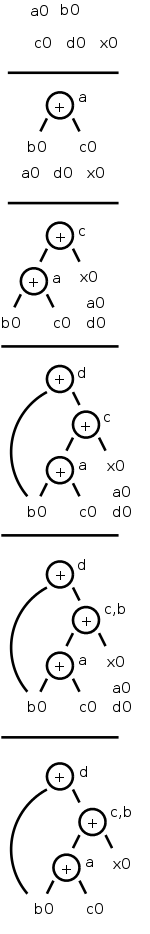
Formally, this is defined as follows.
- Create a leaf for the initial value of each variable appearing
in the block.
(We do not know what that the value is, not even if the variable
has ever been given a value).
- Create a node N for each statement s in the block.
- Label N with the operator of s.
This label is drawn inside the node.
- Attach to N those variables for which N is the last def in
the block.
These additional labels are drawn along side of N.
- Draw edges from N to each statement that is the last def of
an operand used by N.
- Designate as output nodes those N whose values are
live on exit
, an officially-mysterious term meaning values
possibly used in another block.
(Determining the live on exit values requires global, i.e.,
inter-block, flow analysis.)
As we shall see in the next few sections various basic-block
optimizations are facilitated by using the DAG.
8.5.2: Finding Local Common Subexpressions
As we create nodes for each statement, proceeding in the static
order of the statements, we might notice that a new node is just
like one already in the DAG in which case we don't need a new node
and can use the old node to compute the new value in addition to the
one it already was computing.
Specifically, we do not construct a new node if an existing node
has the same children in the same order and is labeled with the same
operation.
Consider computing the DAG for the following block of code.
    a = b + c
    c = a + x
    d = b + c
    b = a + x
The DAG construction proceeds as follows (the movie on the right
accompanies the explanation).
- First we construct leaves with the initial values.
- Next we process a = b + c.
This produces a node labeled + with a attached and having
b0 and c0 as children.
- Next we process c = a + x.
- Next we process d = b + c.
Although we have already computed b + c in the first statement,
the c's are not the same, so we produce a new node.
- Then we process b = a + x.
Since we have already computed a + x in statement 2, we do not
produce a new node, but instead attach b to the old node.
- Finally, we tidy up and erase the unused initial values.
You might think that with only three computation nodes in the DAG,
the block could be reduced to three statements (dropping the
computation of b).
However, this is wrong.
Only if b is dead on exit can we omit the computation of b.
We can, however, replace the last statement with the simpler
b = c.
Sometimes a combination of techniques finds improvements that no
single technique would find.
For example if a-b is computed, then both a and b are incremented by
one, and then a-b is computed again, it will not be recognized as a
common subexpression even though the value has not changed.
However, when combined with various algebraic transformations, the
common value can be recognized.
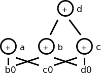
8.5.3: Dead Code Elimination
Assume we are told (by global flow analysis) that certain values
are dead on exit.
We examine each root (node with no ancestor) and delete any for
which all attached variables are dead on exit.
This process is repeated since new roots may have appeared.
For example, if we are told, for the picture on the right, that c
and d are dead on exit, then the root d can be removed since d is
dead.
Then the rightmost node becomes a root, which also can be removed
(since c is dead).
8.5.4: The Use of Algebraic Identities
Some of these are quite clear.
We can of course replace x+0 or 0+x by simply x.
Similar considerations apply to 1*x, x*1, x-0, and x/1.
Another class of simplifications is strength reduction,
where we replace one operation by a cheaper one.
A simple example is replacing 2*x by x+x on architectures where
addition is cheaper than multiplication.
A more sophisticated strength reduction is applied by compilers that
recognize induction variables
(loop indices).
Inside a
for i from 1 to N
loop, the expression 4*i can be strength reduced to j=j+4 and 2^i
can be strength reduced to j=2*j (with suitable initializations of j
just before the loop).
Other uses of algebraic identities are possible; many require a
careful reading of the language reference manual to ensure their
legality.
For example, even though it might be advantageous to convert
((a + b) * f(x)) * a
to
((a + b) * a) * f(x)
it is illegal in Fortran since the programmer's use of parentheses
to specify the order of operations can not be violated.
Does
    a = b + c
    x = y + c + b + r
contain a common subexpression of b+c that need be evaluated only
once?
The answer depends on whether the language permits the use of the
associative and commutative law for addition.
(Note that the associative law is invalid for floating point numbers.)
8.5.5: Representation of Array References
Arrays are tricky.
Question: Does
    x = a[i]
    a[j] = y
    z = a[i]
contain a common subexpression of a[i] that need be evaluated only
once?
The answer depends on whether i=j.
Without some form of disambiguation, we can not be assured that the
values of i and j are distinct.
Thus we must support the worst case condition that i=j and hence the
two evaluations of a[i] must each be performed.
A statement of the form x = a[i] generates a node labeled with the
operator =[] and the variable x, and having children a0,
the initial value of a, and the value of i.
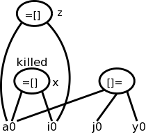
A statement of the form a[j] = y generates a node labeled with
operator []= and three children a0. j, and y, but with no
variable as label.
The new feature is that this node kills all existing nodes depending
on a0.
A killed node can not received any future labels so cannot becomew a
common subexpression.
Returning to our example
    x = a[i]
    a[j] = y
    z = a[i]
We obtain the top figure to the right.
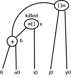
Sometimes it is not children but grandchildren (or other
descendant) that are arrays.
For example we might have
    b = a + 8    // b[i] is 8 bytes past a[i]
    x = b[i]
    b[j] = y
We are using C-like semantics, where an array references is thought
to be a pointer to a[0], the first element of the array.
Hence b is a pointer to 8 bytes past the first element of a, which
is a[2] for an integer array and a[1] for a real array.
Again we need to have the third statement kill the second node even
though the actual array (a) is a grandchild.
This is shown in the bottom figure.
8.5.6: Pointer Assignment and Procedure Calls
Pointers are even trickier than arrays.
Together they have spawned a mini-industry in disambiguation
,
i.e., when can we tell whether two array or pointer references refer
to the same or different locations.
A trivial case of disambiguation occurs with.
    p = &x
    *p = y
In this case we know precisely the value of p so the second
statement kills only nodes with x attached.
With no disambiguation information, we must assume
that a pointer can refer to any location.
Consider
    x = *p
    *q = y
We must treat the first statement as a use of every variable;
pictorially the =* operator takes all current nodes with identifiers
as arguments.
This impacts dead code elimination.
We must treat the second statement as writing every variable.
That is all existing nodes are killed, which impacts common
subexpression elimination.
In our basic-block level approach, a procedure call has properties
similar to a pointer reference:
For all x in the scope of P, we must
treat a call of P as using all nodes with x attached and also
killing those same nodes.
8.5.7: Reassembling Basic Blocks From DAGs
Now that we have improved the DAG for a basic block, we need to
regenerate the quads.
That is, we need to obtain the sequence of quads corresponding to
the new DAG.
We need to construct a quad for every node that has a variable
attached.
If there are several variables attached we chose a live-on-exit
variable, assuming we have done the necessary global flow analysis
to determine such variables).
If there are several live-on-exit variables we need to compute one
and make a copy so that we have both.
An optimization pass may eliminate the copy if it is able to assure
that one such variable may be used whenever the other is
referenced.
Example
Recall the example from our movie
    a = b + c
    c = a + x
    d = b + c
    b = a + x
If b is dead on exit, the first three instructions suffice.
If not we produce instead
    a = b + c
    c = a + x
    d = b + c
    b = c
which is still an improvement as the copy instruction is less
expensive than the addition on most architectures.
If global analysis shows that, whenever this definition of b is
used, c contains the same value, we can eliminate the copy and use c
in place of b.
Order of Generated Instructions
Note that of the following 5 rules, 2 are due to arrays, and 2 due
to pointers.
- The DAG order must be respected (defs before uses).
- Assignment to an array must follow all assignments to or uses
of the same array that preceded it in the original block (no
reordering of array assignments).
- Uses of an array must follow all (preceding according to the
original block) assignments to it; so the only transformation
possible is reordering uses.
- All variable references must follow all (preceding ...)
procedure calls or assignment through a pointer.
- A procedure call or assignment through a pointer must follow all
(preceding ...) variable references.
Homework: 1, 2,
8.6: A Simple Code Generator
A big issue is proper use of the registers, which are often in
short supply, and which are used/required for several purposes.
- Some operands must be in registers.
- Holding temporaries (i.e., values used in only one basic
block) thereby avoiding expensive memory ops.
- Holding inter-basic-block values (loop index).
- Storage management (e.g., stack pointer).
For this section we assume a RISC architecture.
Specifically, we assume only loads and stores touch memory;
that is, the instruction set consists of
    LD  reg, mem
    ST  mem, reg
    OP  reg, reg, reg
where there is one OP for each operation type used in the three
address code.
We will not consider the use of constants so we need not consider if
constants can be used in place of registers.
A major simplification is we assume that, for each three address
operation, there is precisely one machine instruction that
accomplishes the task.
This eliminates the question of instruction selection.
We do, however, consider register usage.
Although we have not done global flow analysis (part of
optimization), we will point out places where live-on-exit
information would help us make better use of the available registers.
Recall that the mem operand in the load LD and store ST
instructions can use any of the previously discussed addressing
modes.
8.6.1: Register and Address Descriptors
These are the primary data structures used by the code generator.
They keep track of what values are in each register as well as where
a given value resides.
- Each register has a register descriptor containing the
list of variables currently stored in this register.
At the start of the basic block all register descriptors are empty.
- Each variable has a address descriptor containing the
list of locations where this variable is currently stored.
Possibilities are its memory location and one or more registers.
The memory location might be in the static area, the stack, or
presumably the heap (but not mentioned in the text).
The register descriptors could be omitted since you can compute
them from the address descriptors.
8.6.2: The Code-Generation Algorithm
There are basically three parts to (this simple algorithm for) code
generation.
- Choosing registers
- Generating instructions
- Managing descriptors
We will isolate register allocation in a function
getReg(Instruction), which is presented later.
First presented is the algorithm to generate instructions.
This algorithm uses getReg() and the descriptors.
Then we learn how to manage the descriptors and finally we study
getReg() itself.
Machine Instructions for Operations
Given a quad OP x, y, z (i.e., x = y OP z), proceed as follows.
- Call getReg(OP x, y, z) to get Rx, Ry, and
Rz, the registers to be used for x, y, and z
respectively.
Note that getReg merely selects the registers, it
does not guarantee that the desired values are present
in these registers.
- Check the register descriptor for Ry.
If y is not present in Ry, check the address descriptor
for y and issue
LD Ry, y'
y' is some location containing y.
Perhaps y is in a register other than Ry.
- Similar treatment for Rz.
- Generate the instruction
OP Rx, Ry, Rz
Note that x now is not in its memory location.
Machine Instructions for Copy Statements
When processing
x = y
steps 1 and 2 are analogous to the above, step 3 is vacuous, and
step 4 is omitted since getReg() will set
Rx=Ry.
Note that if y was already in a register before the copy
instruction, no code is generated at this point
(getReg will choose Ry to be a register containing y).
Also note that since the value of x is now not in
its memory location, we may need to store this value into x at block
exit.
Ending the Basic Block
You may have noticed that we have not yet generated any store
instructions.
They occur here (and during spill code in getReg()).
We need to ensure that all variables needed by (dynamically)
subsequent blocks (i.e., those live-on-exit) have their current
values in their memory locations.
- Temporaries are never live beyond a basic block so can be
ignored.
- Variables dead on exit (thank you global flow analysis for
determining such variables) are also ignored.
- All live on exit variables (for all non-temporaries) need
to be in their memory location on exit from the block.
Therefore, for any live on exit variable whose own memory
location is not listed in its address descriptor, generate
ST x, R where R is a register listed in the
address descriptor.
Managing Register and Address Descriptors
This is fairly clear.
We just have to think through what happens when we do a load, a
store, an (assembler) OP, or a copy.
For R a register, let Desc(R) be its register descriptor.
For x a program variable, let Desc(x) be its address descriptor.
- Load: LD R, x
- Desc(R) = x (removing everything else from Desc(R))
- Add R to Desc(x) (leaving alone everything else in Desc(x))
- Remove R from Desc(w) for all w ≠ x
(not in 2e please check)
- Store: ST x, R
- Add the memory location of x to Desc(x)
- Operation: OP Rx, Ry, Rz
implementing the quad OP x, y, z
- Desc(Rx) = x
- Desc(x) = Rx (Now Desc(x) does not
contain x's memory location!)
- Remove Rx from Desc(w) for all w ≠ x
- Copy: For x = y after processing the load (if needed)
- Add x to Desc(Ry)
(recall that Ry=Rx).
- Desc(x) = Ry.
Example
Since we haven't specified getReg() yet, we will assume there are
an unlimited number of registers so we do not need to generate any
spill code (saving the register's value in memory).
One of getReg()'s jobs is to generate spill code when a register needs
to be used for another purpose and the current value is not
presently in memory.
Despite having ample registers and thus not generating spill code,
we will not be wasteful of registers.
- When a register holds a temporary value and there are no
subsequent uses of this value, we reuse that register.
- When a register holds the value of a program variable and
there are no subsequent uses of this value, we reuse that
register providing this value is also in the
memory location for the variable.
- When a register holds the value of a program variable and all
subsequent uses of this value are preceded by a redefinition, we
could reuse this register.
But to know about all subsequent uses may require
live/dead-on-exit knowledge.
This example is from the book.
I give another example after presenting getReg(), that I believe
justifies my claim that the book is missing an action for load
instructions, as indicated above.
Assume a, b, c, and d are program variables and t, u, v are
compiler generated temporaries (I would call these t$1, t$2, and
t$3).
The intermediate language program is in the middle with the generated
code for each quad shown.
To the right is shown the contents of all the descriptors.
The code generation is explained on the left.
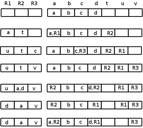
t = a - b
    LD  R1, a
    LD  R2, b
    SUB R2, R1, R2

u = a - c
    LD  r3, c
    SUB R1, R1, R3

v = t + u
    ADD R3, R2, R1

a = d
    LD  R2, d

d = v + u
    ADD R1, R3, R1

exit
    ST  a, R2
    ST  d, R1
- For the first quad, we need all three instructions since nothing
is register resident on block entry.
Since b is not used again, we can reuse its register.
(Note that the current value of b is in its memory location.)
- We do not load a again since its value is R1, which we can reuse
for u since a is not used below.
- We again reuse a register for the result; this time because c is
not used again.
- The copy instruction required a load since d was not in a
register.
As the descriptor shows, a was assigned to the same register, but
no machine instruction was required.
- The last instruction uses values already in registers.
We can reuse R1 since u is a temporary.
- At block exit, lacking global flow analysis, we must assume all
program variables are live and hence must store back to memory any
values located only in registers.
8.6.3: Design of the Function getReg
Consider
x = y OP z
Picking registers for y and z are the same; we just do y.
Choosing a register for x is a little different.
A copy instruction
x = y
is easier.
Choosing Ry
Similar to demand paging, where the goal is to produce an available
frame, our objective here is to produce an available register we can
use for Ry.
We apply the following steps in order until one succeeds.
(Step 2 is a special case of step 3.)
- If Desc(y) contains a register, use of these for Ry.
- If Desc(R) is empty for some registers, pick one of these.
- Pick a register for which the cleaning procedure
generates a minimal number of store instructions.
To clean an in-use register R do the following for each v in Desc(R).
- If Desc(v) includes something besides R, no store is needed
for v.
- If v is x and x is not z, no store is needed since x is
being overwritten.
- No store is needed if there is no further use of v prior to
a redefinition.
This is easy to check for further uses within the block.
If v is live on exit (e.g., we have no global flow analysis),
we need a redefinition later in this block.
- Otherwise a spill ST v, R is generated.
Choosing Rz and Rx, and Processing x = y
As stated above choosing Rz is the same as choosing
Ry.
Choosing Rx has the following differences.
- Since Rx will be written it is not enough for
Desc(x) to contain a register R as in 1. above;
instead, Desc(R) must contain only x.
- If there is no further use of y prior to a redefinition (as
described above for v) and if Ry contains only y (or
will do so after it is loaded), then Ry can be used
for Rx.
Similarly, Rz might be usable for Rx.
getReg(x=y) chooses Ry as above and chooses
Rx=Ry.
Example
                               R1  R2  R3    a    b    c    d    e
                                             a    b    c    d    e
    a = b + c
        LD  R1, b
        LD  R2, c
        ADD R3, R1, R2
                               R1  R2  R3    a    b    c    d    e
                               b   c   a     R3  b,R1 c,R2  d    e
    d = a + e
        LD  R1, e
        ADD R2, R3, R1
                              R1  R2  R3    a    b    c    d    e
                       2e →   e   d   a     R3  b,R1  c    R2  e,R1
                       me →   e   d   a     R3   b    c    R2  e,R1
We needed registers for d and e; none were free.
getReg() first chose R2 for d since R2's current contents, the value
of c, was also located in memory.
getReg() then chose R1 for e for the same reason.
Using the 2e algorithm, b might appear to be in R1
(depends if you look in the address or register descriptors).
    a = e + d
        ADD R3, R1, R2
                              Descriptors unchanged

    e = a + b
        ADD R1, R3, R1   ← possible wrong answer from 2e
                              R1  R2  R3    a    b    c    d    e
                              e   d    a    R3  b,R1  c    R2   R1

        LD  R1, b
        ADD R1, R3, R1
                              R1  R2  R3    a    b    c    d    e
                              e   d    a    R3   b    c    R2   R1
The 2e might think R1 has b (address descriptor) and also
conclude R1 has only e (register descriptor) so might generate the
erroneous code shown.
Really b is not in a register so must be loaded.
R3 has the value of a so was already chosen for a.
R2 or R1 could be chosen.
If R2 was chosen, we would need to spill d (we must assume live-on-exit,
since we have no global flow analysis).
We choose R1 since no spill is needed: the value of e (the current
occupant of R1) is also in its memory location.
  exit
      ST  a, R3
      ST  d, R2
      ST  e, R1
8.7: Peephole Optimization
8.8: Register Allocation and Assignment
8.9: Instruction Selection by Tree Rewriting
What if a given quad needs several OPs and we have choices?
We would like to be able to describe the machine OPs in a way that
enables us to find a sequence of OPs (and LDs and STs) to do the job.
The idea is that you express the quad as a tree and express each OP
as a (sub-)tree simplification, i.e. the op replaces a subtree by a
simpler subtree.
In fact the simpler subtree is just a single node.
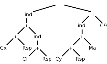
The diagram on the right represents x[i] = y[a] + 9,
where x and y are on the stack and a is in the static area.
M's are values in memory; C's are constants; and R's are registers.
The weird ind (presumably short for indirect) treats its argument as
a memory location.
Compare this to grammars:
A production replaces the RHS by the LHS.
We consider context free grammars where the LHS is a single
nonterminal.
For example, a LD replaces a Memory node with a Register node.
Another example is that
ADD Ri, Ri, Rj
replaces a subtree consisting of a + with both children registers (i
and j) with a Register node (i).
As you do the pattern matching and reductions (apply the
productions), you emit the corresponding code (semantic actions).
So to support a new processor, you need to supply the tree
transformations corresponding to every instruction in the
instruction set.
8.10: Optimal Code Generation for Expressions
This is quite cute.
We assume all operators are binary and label the instruction tree
with something like the height.
This gives the minimum number of registers needed so that no spill
code is required.
A few details follow.
8.10.1: Ershov Numbers
- Draw the
expression tree
, the abstract syntax tree for an
expression.
- Label the leaves with 1.
- Label interior nodes with L:
- If the children have the same label x, L=x+1.
This looks like height.
- If the children have different labels, x and y, L=max(x,y).
8.10.2: Generating Code From Labeled Expression Trees
- Recursive algorithm starting at the root.
Each node puts its answer in the highest number register it is
assigned.
The idea is that a node uses (mostly) the same registers as its
sibling.
- If the labels on the children are equal to L, the parent's
label is L+1.
- Give one child L regs ending in highest assigned to
parent.
Note that the lowest reg assigned to the parent is not
used by this child.
The answer appears in top reg assigned to the child, which
is the top reg assigned to the parent.
- Give other child L regs, ending one below the top reg
assigned to the parent.
This child does use the bottom reg assigned to the parent.
The answer appears in top reg assigned to the child, i.e.,
the penultimate parent reg.
- Parent uses a two address OP to compute its answer in the
same reg used by first child, which is the top reg
assigned to the parent.
- If the labels on the children are M<L, the parent is
labeled L.
- Give
bigger
child all L parent regs.
- Give other child M regs ending one below bigger child.
- Parent uses 2-addr OP computing answer in L
- If at a leaf (operand), load it into assigned reg.
Can see this is optimal (assuming you have enough registers).
- Loads each operand only once.
- Performs each operation only once.
- Does no stores.
- Minimal number of registers having the above three properties.
- Show need L registers to produce a result with label L.
- Must compute one side and not use the register containing
its answer before finishing the other side.
- Apply this argument recursively.
8.10.3: Evaluating Expressions with an Insufficient Supply of Registers
Rough idea is to apply the above recursive algorithm, but at each
recursive step, if the number of regs is not enough, store the
result of the first child computed before starting the second.
8.11: Dynamic Programming Code-Generation
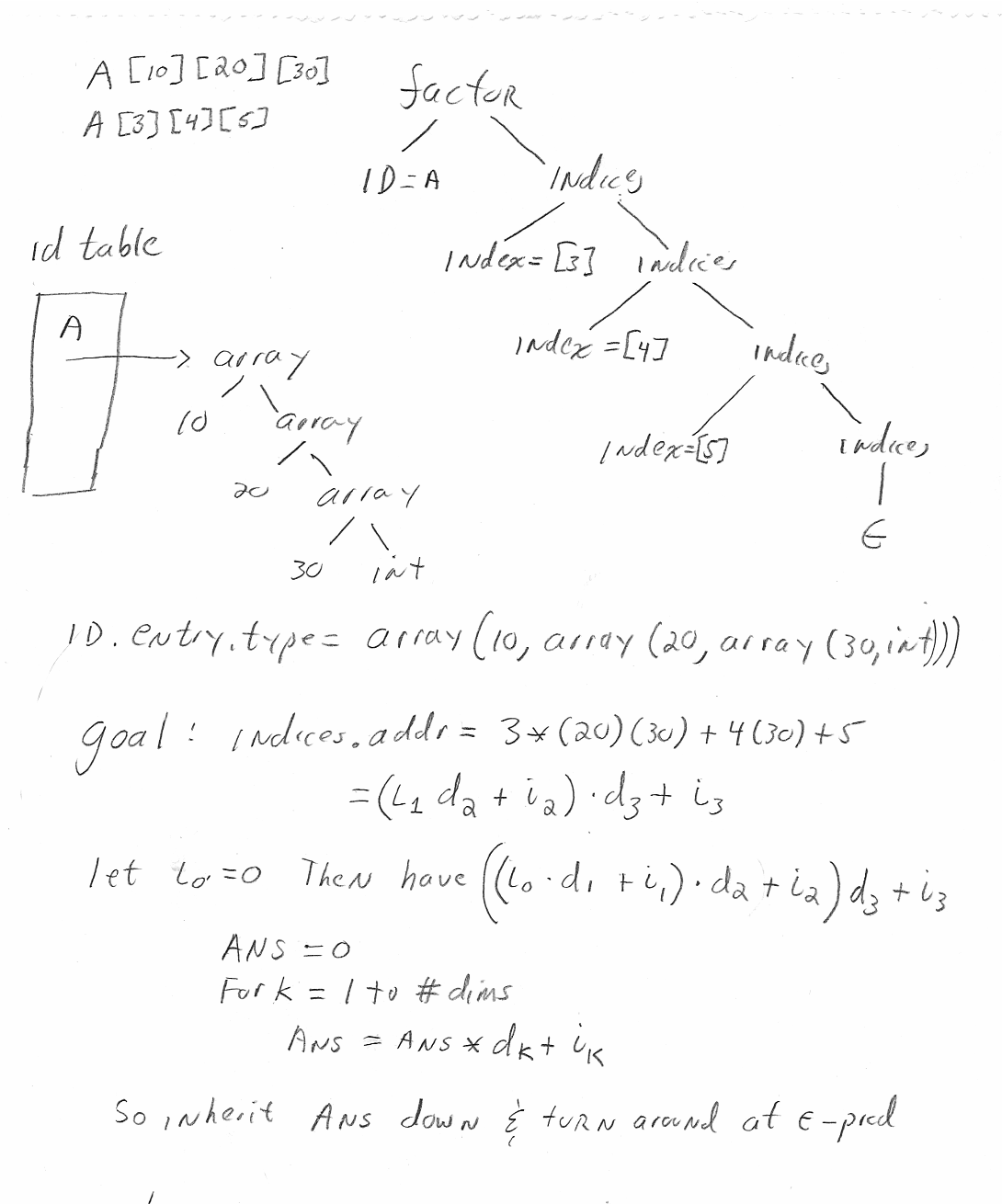