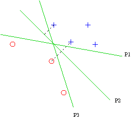
Consider a classification problem of determining whether an instance X is a member of one particular category C. That is, the classification attribute has two values T and F.
Suppose that all the predictive attributes are numerical. Thus, an instance X can be considered to be a vector < X1 ... Xk > where the Xi are all numbers.
The simplest kind of classifier for this case is a linear classifier which is a vector of k weights < W1 ... Wk > and a threshhold T with the following rule:
If W1X1 + W2X2 + ... + WkXk > T then predict X.C=T else predict X.C=F.
For fixed W1 ... Wk,
the equation
W1X1 +
W2X2 + ... +
WkXk = T defines a hyperplane in the k-dimensional space
of values of X1 ... Xk.
All points on one side of the hyperplane obey the equation
W1X1 +
W2X2 + ... +
WkXk > T
and are judged to be in category C.
All points on the other side of the hyperplane obey the equation
W1X1 +
W2X2 + ... +
WkXk < T
and are judged to be outside category C.
log(P(I.A1= x1 | I.C=T)) + log(P(I.A2= x2 | I.C=T)) + ... + log(P(I.Ak= xk | I.C=T)) + log(P(I.C=T)) >
log(P(I.A1= x1 | I.C=F)) + log(P(I.A2= x2 | I.C=F)) + ... + log(P(I.Ak= xk | I.C=F)) + log(P(I.C=F))
However, this is equivalent to
(1/2) [log(P(I.A1=1 | I.C=T)) + log(P(I.A1=-1 | I.C=F)) - log(P(I.A1=1 | I.C=F)) - log(P(I.A1=-1| I.C=T))] x1 + ... +which is a linear inequality in x1 ... xk
(1/2) [log(P(I.Ak=1 | I.C=T)) + log(P(I.Ak=-1 | I.C=F)) - log(P(I.Ak=1 | I.C=F)) - log(P(I.Ak=-1| I.C=T))] xk
>
log(P(I.C=F)) - log(P(I.C=T)) +
(1/2) [log(P(I.A1=1 | I.C=T)) + log(P(I.A1=1 | I.C=F)) - log(P(I.A1=-1 | I.C=F)) - log(P(I.A1=-1| I.C=T))] + ... +
(1/2) [log(P(I.Ak=1 | I.C=T)) + log(P(I.Ak=1 | I.C=F)) - log(P(I.Ak=-1 | I.C=F)) - log(P(I.Ak=-1| I.C=T))]
The Naive Bayes multinomial model of text can also be viewed as a linear
separator. Suppose the text T is "A rose is a rose is a rose". The Naive
Bayes method states that to decide whether T is a member of category C
seeing whether
log(P("a"|C)) + log(P("rose"|C)) + log(P("is"|C)) + log(P("a"|C)) +
log(P("rose"|C)) + log(P(C)) >
log(P("a"|~C)) + log(P("rose"|~C)) + log(P("is"|~C)) +
log(P("a"|~C)) + log(P("rose"|~C)) + log(P(~C))
Equivalently,
[log(P("a"|C) - log(P("a"|~C)] * 3 +
[log(P("rose"|C) - log(P("rose"|~C)] * 3 +
[log(P("is"|C) - log(P("is"|~C)] * 2 >
[log(P(~C)) - log(P(C))]
Therefore: let us consider a vector space in which each word in the language is a dimension, and let us say a document D corresponds to a vector V such that the coordinate of D in the dimension corresponding to word U is the number of occurrences of U in D (3 for "a" and "rose", 2 for "is"). Then the Naive Bayes classifier is a linear discriminator where the weight WU for the dimension corresponding to U is equal to log(P(U|C)) - log(P(U|~C)) and the threshhold is log(P(~C)) - log(P(C)).
The Bernoulli model for Naive Bayes can also be construed as a linear separator; I leave that as an exercise.
"No one ever got fired for using an SVM."
Introduction to Information Retrieval by Christopher Manning,
Prabhakar Raghavan, and Hinrich Schutze, Cambridge U. Press, 2008
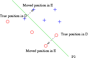
Suppose that hyperplane P is a linear separator for a labelled data set D. The margin of P is the minimal distance from any element in D to P. The SVM of D is the hyperplane P with maximal margin.

The SVM generally predicts unseen points more accurately than any other linear classifiers, because it requires that any future point classified as C must be quite far from any point labelled as not C. (There are also more sophisticated and cogent arguments for this conclusion.)
With a little algebra, one can express the problem of finding the SVM as a problem of minimizing a quadratic function subject to linear constraints. (Essentially, the distance squared is a quadratic function on W and T and the constraint that all the points are correctly categorized is a set of linear constraints on W and T, though it takes a little munging to make this come out neatly.) This is a well-known optimization problem.
