A brief explanation of our model
We demonstrate how our model works
by the following simple example. Note that this is a very simple demonstration of the basic framework
of our model. The actual implementation in our software package does not strictly follow this demonstration.
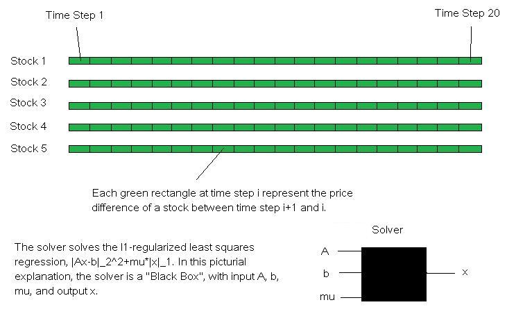
Our model aims at finding x such that x minimizes
|Ax-b|_2^2+mu*|x|_1, and then use this x for prediction. A and b are determined by the data and the size of the sliding
window, and mu is either input by the user, trained by train_model.m if the solver is not 'path-finding'. If the solver
is 'path-finding', then mu is ignored.
Suppose we have 20 stock price differenctial data for 5 stocks. We're
interested in predicting the differential prices (which is close to predicting the returns) for stock 1
starting at time step 21. We'll use a sliding window size 10. That is, we'll use the value of the time
series from time step i-10 to i to predict the price difference at time step i+1 for stock 1. We will
always use mu=0.03. We will use the solver 'l1_ls' which solves . We don't remove the target series (i.e stock 1) when
we do prediction because we assume that stock 1 also linearly depends on a shifted copy of itself.
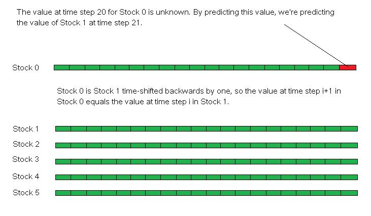
Now we initialize our model: We first
make a copy of stock 1 (the stock we're interested in prediction). Then We shift stock 1 backwards by one time step, discarding its first value. So at
the last time step (time step 20), the value of the target series (from now on, we call it stock 0) at
time step 20 is the value of stock 1 at time step 21, which is of course unknown. But we can use the solver
to predict the value of stock 0 at time step 20. This predicted value will be the predicted value of stock 1
at time step 21.
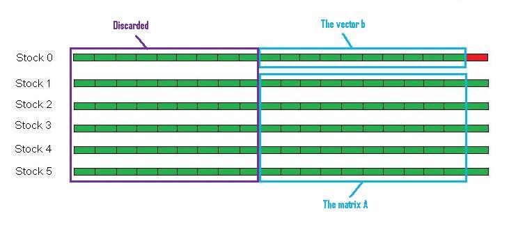
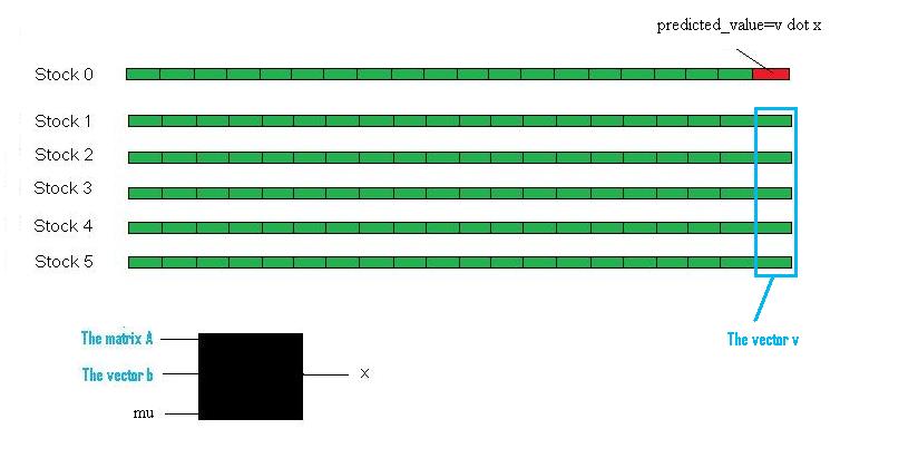
Next, we feed the matrix A, the vector b,
and the mu to the solver. We take the values of Stock 1 through Stock 5 from time step 20-10=10 to 20-1=19. This
matrix will be our A. Then we take the values of Stock 0 from time step 20-10=10 to 20-1=19. This vector will
be b. The mu value is fixed in our example (although in reality, mu should be frequently trained). We feed these
parameters to the "Black Box" and get back an X. Notice that the number of time steps in A equals the sliding
window size 10.
In our model, we assume that there exists a
sparse linear correlation between Stock 0 and Stock 1 through Stock 5. Previous step gives us such a sparse linear
correlation vector x, so in this step, we will use this x to predict the value of stock 0 at time step 20. It is
simple: Treat the values of Stock 1 through Stock 5 at time step 20 as a vector. The dot product of this vector with
x is the predicted value for Stock 0 at time step 20. This value is also the predicted value of Stock 1 at time step 21.
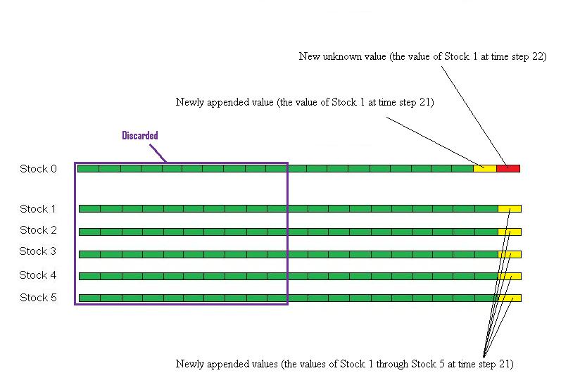
Finally, after we recieve the values of the stocks
at time step 21, we update our model: We discard the values in Stock 0 through Stock 5 at time step 9+1=10. We append the
new values to the end of Stock 1 through Stock 5. We also make a copy of the new value for Stock 1 and append it to the end
of Stock 0. Next time when we want to predict the value of Stock 0 at time step 22, we take the values between time step 11 to
time step 20 in Stock 1 through Stock 5 as A, the values between time step 11 and time step 20 in Stock 0 as b, and
the mu input by the user, and repeat the above procedure for prediction.