Sections Data Structure Search Insert Delete References Visualize Tree operations Algorithm Visualization Homepage

Binary Search Trees Binary search trees store collections of items that can be ordered, such as integers. Binary search trees support the following standard operations. search(x): determines is an item x contained in the tree (and if so returns the item). insert(x): adds item x to the collection stored in the tree, if it is not already there. delete(x): removes item x from the collection stored in the tree. Data structures supporting these operations are called Dictionaries. A simple implementation is to store the items in sorted order in an array. Search(x) is simply a binary search. However, insert(x) and delete(x) are inefficient as, in general, they may require many items to be shifted. 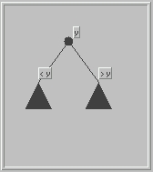Data Structure A potentially more efficient implementation is provided by a binary search tree. There, some item, is stored at the root, y say. 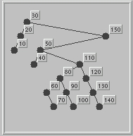Smaller items are organized recursively in the left subtree, larger items in the right subtree: For a given collection of elements, there are many possible search trees. This illustration shows a search tree with 15 nodes. It's a useful exercise to convince oneself that the search tree property stated above holds at every node. Search(x) The implementation of search(x) is straight forward. We start at the root of the tree. Case 1 the tree is empty: then x is not present. Case 2 x = y (the item at the root): then the item y, at the root is returned Case 3 x < y : recursively search the left subtree. 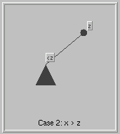Case 4 x > y : recursively search the right subtree. See a visualization. In the description of insert(x) and delete(x) it is convenient to refer to a node by the item it stores; thus y means item y and the node storing y, according to the context; we may write node y to avoid ambiguity. Insert(x) Insert(x) is also simple. See a visualization. 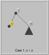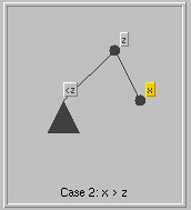Step 1: search(x) Step 2: If x is already in the tree then the insert is already done. Otherwise, the search has found a node z say, and node z has at least one empty subtree; further the search for x continued in this empty subtree, unsuccessfully, of cause. In each case, a new node storing x is added as the appropriate child of z: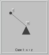 Delete(x) Delete(x) is a little less straightforward. See a visualization. Step 1: search(x) if x is not in the tree, the operation is already done. Otherwise, the goal of steps 2 and 3 is to move item x to a node with only one child. If node x is a leaf or has just one child continue with step 4. 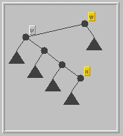Otherwise, Step 2: locate w, the predecessor of x. w is stored at the following location: The rightmost descendant of the left child v of x. To get there, follow right child links from v until a node with no right child is reached; this is node w (it may be that v = w).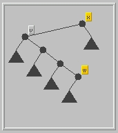 Step 3: Swap items x and w. Temporarily, the data structure is no longer a binary search tree (why?). 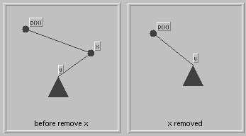Step 4: Remove node x. Simply replace x and its single subtree by the subtree. We need to consider the case for a single right subtree and a single left subtree separately. Our illustrations show x as a right child of p(x); however, there are cases where x is a child child. Case 1: Case 2: The case in which x is a leaf is particularly simple and is left to the reader. References [1] Data Structures and Their Algorithms, Lewis and Denenberg, Harper Collins, 1991, pp 243-251. [2] "Self-adjusting Binary Search Trees", Sleator and Tarjan, JACM Volume 32, No 3, July 1985, pp 652-686. [3] Data Structure and Algorithm Analysis, Mark Weiss, Benjamin Cummins, 1992, pp 119-130. [4] Data Structures, Algorithms, and Performance, Derick Wood, Addison-Wesley, 1993, pp 367-375